Dept. of Computer Science & Eng., Michigan State University, East Lansing, MI, U.S.A.. â . Dept. of Brain ... puted for each assigned class label to facilitate the learning process; (iii) ..... of MIR Flickr dataset is below 77%, while the best AUC re- sults for ..... framework for online milti-class learning with partial feed- back.
Multi-label Learning with Incomplete Class Assignments Serhat Selcuk Bucak∗ Rong Jin∗ Anil K. Jain∗† ∗ Dept. of Computer Science & Eng., Michigan State University, East Lansing, MI, U.S.A. † Dept. of Brain & Cognitive Eng., Korea University, Anam-dong, Seoul, Korea {bucakser,rongjin,jain}@cse.msu.edu
Abstract We consider a special type of multi-label learning where class assignments of training examples are incomplete. As an example, an instance whose true class assignment is (c1 , c2 , c3 ) is only assigned to class c1 when it is used as a training sample. We refer to this problem as multi-label learning with incomplete class assignment. Incompletely labeled data is frequently encountered when the number of classes is very large (hundreds as in MIR Flickr dataset) or when there is a large ambiguity between classes (e.g., jet vs plane). In both cases, it is difficult for users to provide complete class assignments for objects. We propose a ranking based multi-label learning framework that explicitly addresses the challenge of learning from incompletely labeled data by exploiting the group lasso technique to combine the ranking errors. We present a learning algorithm that is empirically shown to be efficient for solving the related optimization problem. Our empirical study shows that the proposed framework is more effective than the state-ofthe-art algorithms for multi-label learning in dealing with incompletely labeled data.
baby, boy, child, eye, face, girl, hair, house, kid, mouth, nose, pink, smile
anime, ball, boy, cartoon, drawing, girl, group, hair, kid, man, people, play, red, sport
Figure 1. Example images from ESP Game dataset and their annotations. The annonations highlighted by bold font, which are used to annotate the same concept/object in the corresponding images, are examples of label ambiguity problem.
frequently encountered in automatic image annotation when the number of classes is very large, and it is only feasible for users to provide limited number of class labels for a given instance. Fig. 1 shows examples of annotated images from the ESP Game. We see some of the annotated words can cause ambiguity. For instance the keywords baby, kid and boy can be used interchangeable, and this can be given as an example of label ambiguity. Note that these annotations are generated by collapsing annotated words from multiple users. It is thus very likely that each individual user only provides incomplete annotation with a few keywords. It is important to distinguish the learning scenario studied in this work from the related ones in the previous studies: (i) partial labeling [23, 18] where for each training instance, only one of its class assignments is correct; (ii) weakly labeled data [24] where confidence score is computed for each assigned class label to facilitate the learning process; (iii) harvesting weakly tagged image databases [9] that focuses on removing false class assignments for training set; (iv) partially labeled data used in the image annotation study [14] that refers to the training images where only a subset of their segments are labeled; (v) bandit multiclass learning [19, 32] that focuses on multi-class learning, where each instance is only assigned to one class.
1. Introduction Multi-label learning is an important problem in machine learning, and has found applications in several computer vision problems (e.g., visual object recognition and automatic image annotation). Many algorithms have been developed for multi-label learning [3, 17, 29, 27, 10, 21, 13]. In this work, we consider the multi-label learning problem in which only a subset of the true class assignments is available for each training instance. As an example, an instance whose true class assignment is (c1 , c2 , c3 ) is only presented with class c1 when it is used for training. Our goal is to learn a multi-labeling model from the training examples with incomplete class assignments. We refer to this problem as multi-label learning with incomplete class assignments, and the training data as incompletely labeled data. Multi-label learning with incomplete class assignments is 2801
There is a rich body of literature on multi-label learning, ranging from the simple approaches that divide multi-label learning into a set of binary classification problems [5] to more sophisticated approaches that explicitly explore the correlation among classes [29, 27, 10, 21] and to multilabel ranking approaches [13, 4, 3, 6, 27, 2] that cast multilabel learning into a ranking problem. But none of these approaches addresses the challenge of multi-label learning from incompletely labeled data, which is a more realistic scenario. To this end, we present a multi-label learning framework based on the idea of multi-label ranking [13, 6, 27, 2]. Unlike the classification approaches that make a binary decision about the class assignment for a given instance, multi-label ranking ranks classes for the given instance such that the “true” classes are ranked before the other classes. By avoiding a binary decision, multilabel ranking is usually more robust than the classification approaches, particularly when the number of classes is very large [29, 2]. In order to handle the problem of incomplete class assignment, we extend multi-label ranking by exploiting the group lasso technique [33] to combine the errors in ranking the assigned classes against the unassigned classes. As will be seen in later discussion, by using group lasso to combine ranking errors, the proposed framework may be able to automatically detect the missed class assignment and consequentially improve the classification accuracy. We present an efficient learning algorithm for the proposed framework. This is important since the naive implementation of multi-label ranking will result in a pairwise comparison between every pair of classes, making it difficult to scale to a large number of classes and training instances. Our empirical studies on three benchmark datasets for image annotation and visual object recognition indicate that (i) our framework is robust to missing class assignments compared to the state-of-the-art approaches for multi-label learning, and (ii) the proposed approach is computationally efficient and scales well to the number of training examples.
However, given the data is only partially labeled, some of the unassigned class labels may indeed be the true classes, and the above loss function for x may overestimate the classification error. To address this issue, we introduce a slack variable, denoted by εk,l , to account for the error of ranking an unassigned class l before the assigned class k. This introduces the following constraint εk,l + fk (x) ≥ 1 + fl (x)
Now, instead adding all the errors together for example �a of �m x, i.e., k=1 l=a+1 εk,l , we combine the ranking errors εk,l via a group lasso regularizer, i.e., � m �� � � a � ε2k,l (3) l=a+1
In order to handle incompletely labeled data, we consider exploring the group lasso regularizer when estimating the error in ranking the assigned classes against the unassigned ones. The key idea is to selectively penalize the ranking errors. To facilitate our discussion, we consider an instance x that is assigned to classes c1 , . . . , ca . Consequently, classes ca+1 , . . . , cm are remained as the unassigned classes for x. If example x is fully labeled, following [2], the ranking error for given classification functions fk (x), k ∈ [m] is expressed as max(0, fl (x) − fk (x) + 1)
k=1
The motivation of using the group lasso for aggregating ranking errors is two fold: first, as stated in the general theory, group lasso is able to select a group of variables, which in our case, is to select the group of ranking errors {εk,l , k = 1, . . . , a} for each unassigned class cl . In particular, an unassigned class cl is likely to be a missing class assignment for example x when many of its ranking errors {εk,l }ak=1 are non-zero, which coincides with the criterion of group selection by group lasso. Thus, by using the group lasso regularizer, we may be able to decide which unassigned class is indeed the missing correct class assignment. Second, group lasso usually results in a sparse solution in which most of the group variables are zero and only a small number of groups are assigned non-zero values. In our case, the sparse solution implies that most of the unassigned classes for x are indeed correct, and only a few unassigned classes are the true class assignments for x that are missed by manual labeling. Let x1 , . . . , xn be the collection of training instances that are labeled by Y1 , . . . , Yn , where each Yi ⊂ Y. For the convenience of presentation, we represent each class i assignment Yi by a binary vector y i = (y1i , . . . , ym ) ∈ {−1, +1}m , where yki = +1 if k ∈ Yi and yki = −1 if k∈ / Yi . Using the group lasso regularizer described above, we have the following optimization problem:
2. A Framework for Multi-label Learning from Incompletely Labeled Data
a m � �
(2)
m n � �� � 1� |fk |2Hκ + C �2 (fk (xi ) − fl (xi )) fk ∈Hκ 2 i=1
min
k=1
l∈Y / i
(4)
k∈Yi
where �(z) = max(0, 1 − z) is the hinge loss function that assesses the error in ranking two classes ck and cl . In the next section, we discuss the strategy for efficiently optimizing Eq. (4).
3. Optimization Algorithm First, we have the following representer theorem for f (x) that optimizes Eq. (4).
(1)
k=1 l=a+1
2802
Theorem 3 The optimal solution f (x) to Eq. (7) can be expressed as follows:
Theorem 1 The optimal solution to Eq. (4) admits the following expression for f (x), i.e., fk (x) =
n �
yki αki κ(x, xi ),
fk (x) =
k = 1, . . . , m
i � where αi = (α1i , . . . , αm ) , i = 1 . . . n is the optimal solution to the following optimization problem: ⎛ ⎞ m n n � � � ⎝ (8) αki − αki αkj yki ykj Ki,j ⎠ maxn i
where αki , i = 1, . . . , n are the combination weights. It is straightforward to verify the above representer theorem. Next, in order to solve Eq. (4) efficiently, we aim to linearize the objective function in Eq. (4) by using the following lemma. �� a �m 2 Lemma 1 l=a+1 k=1 � (fk (xi ) − fl (xi )) is equivalent to the following expression: � m a � � i γk,l �(fk (xi ) − fl (xi )) (5) max s.t.
l=a+1 k=1 i max |γ·,l |2 1≤l≤m−a
≤1
{α ∈Ωi }i=1
The proof of this theorem can be found in Appendix A. Note that although the objective function in Eq. (8) is similar to that of SVM, it is the constraints specified in domain Ωi that makes this problem computationally more challenging. In order to efficiently solve Eq. (8), we consider the block coordinate descent method. In particular, we aim to optimize αi with the other {αj , j �= i} being fixed. Without a loss of generality, we assume that example xi is assigned to the first a classes and is not assigned to the remaining b = m − a classes. For the convenience of presentation, we drop the index i and write αi as α. We thus have the following optimization problem for αi .
(6)
max α∈Ω
Theorem 2 The problem in Eq. (4) is equivalent to the following convex-concave optimization problem
{γ ∈Δi }i=1 {fk ∈Hκ }k=1
+C
n � � �
(7)
⎪ ⎩
γ i ∈ Rm×m
1≤l≤m
αk2 − 2
k=1
m �
yk αk
k=1
� j�=i
αkj ykj Ki,j (9)
In the above, we use the notation αi:j = (αi , . . . , αj ) to represent a subset of vector α whose index ranges from i to j. 1a represents a vector of a dimensions with all its elements being one. We now aim to simplify the problem in Eq. (9). First, we have for any α ∈ Ω
i where γ i = [γk,l ]m×m and
Δi =
m �
s.t. α1:a = Cγ1b , αa+1:a+b = Cγ � 1a }
i γk,l �(fk (xi ) − fl (xi ))
i ≥ 0, k, l = 1, . . . , m, γk,l i γ / Yi , : k,l = 0 if l ∈ Yi or k ∈ i |2 ≤ 1 max |γ·,l
αk − Ki,i
k=1
k=1
i=1 l∈Y / i k∈Yi
⎧ ⎪ ⎨
m �
where Ω is defined as � Ω = α ∈ Rm : ∃γ ∈ Ra×b + , |γ·,l |2 ≤ 1, l ∈ [b]
m
1� |fk |2Hκ 2
i,j=1
� � Ωi = αi ∈ Rm : ∃γ i ∈ Δi s. t. αi = Cγ i 1 + C[γ i ]� 1
Lemma �1� follows directly from the fact that � m a 2 l=a+1 k=1 � (fk (xi ) − fl (xi )) is a L1,2 norm of the loss function �(fk (x) − fl (x)) and the dual norm of L1,2 is L∞,2 . Using lemma 1, we turn Eq. (4) into a convex-concave optimization problem as revealed in the following theorem.
min m L =
i=1
k=1
where
where γ·,l stands for the lth column vector of matrix γ i .
max n i
yki αki κ(x, xi )
i=1
i=1
γ i ∈Ra×(m−a)
n �
⎫ ⎪ ⎬
m �
⎪ ⎭
αk = 2C(1� a γ1b )
(10)
k=1
Second, we have
The above theorem follows by directly plugging the result of Lemma 1 into Eq. (4). As indicated by the above theorem, the introduction of the group lasso is equivalent to i introducing a different weight γk,l for each comparison between an assigned class and an unassigned class. It is the introduction of these weights that allows us to determine which unassigned class is missed in the user’s annotation.
m � k=1
αk2 =
a � k=1
αk2 +
a+b �
� � � � � (11) αk2 = C 2 1� b γ γ1b + 1a γγ 1a
k=a+1
To simplify the last term in Eq. (9), we define � j j fk−i (xi ) = yk αk yk κ(xi , xj ) j�=i
2803
(12)
and vector f −i = (f1−i (xi ), . . . , fi−i (xi )) = (fa−i , fb−i ). Using these notations, the third term in Eq. (9) becomes m �
αk fk−i (xi ) = α� f −i = Ctr
��
Table 1. Dataset statistics
� � 1b [fa−i ]� + fb−i 1� (13) a] γ
k=1
VOC07 ESP Game MIR Flickr
# samples 9963 10457 10199
# classes 20 268 457
avg. label/img 1.47 6.41 5.30
avg img/label 729.85 250.29 118.43
Thus, we have the following optimization problem to solve � � � � 1 � � max 1� a γ1b − CKi,i 1b γ γ1b + 1a γγ 1a γ∈Δ 2 � � �� −i � γ −tr fb−i 1� a + 1b [fa ]
fewer than five classes form ESP Game dataset. The dataset statistics are given in Table 1. For both datasets, we randomly take 75% of the examples to form the training set and use the rest for testing. We repeat the experiments ten : |γ·,l |2 ≤ 1, l = 1, . . . , b}. The where Δ = {γ ∈ Ra×b times, each with a random partitioning of data for training + problem in Eq. (14) is indeed a Second Order Cone Proand testing, and report the performance averaged over the gramming (SOCP) problem [1]. Although a SOCP probten trials. The bag-of-words model based on dense samlem can be solved by a standard tool like SeDuMi [28], it pling, provided by [11] and [12], is used for image reprecan still be computationally expensive to solve a large-scale sentation. To simulate the situation of incomplete class asSOCP problem. We thus further simplify Eq. (14) by the signment, we conduct experiments in four different settings following approximation for ESP Game and MIR Flickr datasets. In the first setting, � � � � � � 1� termed case-1, there is no missing class assignment for any b γ γ1b + 1a γγ 1a ≈ ηtr(γ γ + γγ ) = 2ηtr(γ γ) (15) training image. In the next three settings, termed case-2, where η > 1 is a parameter introduced for approximation. case-3, and case-4, for each training image, we randomly Using the approximation in Eq. (15), we have choose 20%, 40%, and 60% of the assigned class labels, � � �� � � −i � −i � max 1a γ1b − CKi,i ηtr(γ γ) − tr fb 1a + 1b [fa ] γ (16) respectively, and remove them from the training data. γ∈Δ In addition to the two multi-labeled datasets, we also include the VOC2007 dataset to show that proposed algorithm Define yields comparable results with the state-of-the-art methods � �� −i � −i � (1b 1� = 2H = (2h1 , . . . , 2hb ). (17) for visual object recognition. The majority of the images in a ) − fb 1a − 1b [fa ] VOC2007 dataset are labeled by a single class, as shown in Lemma 2 shows a closed form solution to Eq. (16). Table 1. This property does not make VOC2007 an ideal dataset for evaluating multi-label learning algorithms. NevLemma 2 The optimal solution to Eq. (16) is ertheless, the performance over VOC2007 dataset will al� � low us to examine if the proposed algorithm is effective for |πG (hs )|2 πG (hs ) γ·,s = min 1, , s = 1, . . . , b, (18) visual object recognition. |πG (hs )|2 CKi,i η Evaluation metric. Since our study is focused on multiwhere G = {z : z ∈ Ra+ } and πG (h) projects vector h into label ranking, we evaluate the results of ranked class labels the domain G. by following the protocol in [2]. In particular, we first rank all the classes for each test image in the descending order of The proof of this lemma can be found in Appendix B. their scores; we then vary the number of predicted classes from 1 to the total number of classes, and compute the ROC 4. Experimental Results curve by calculating true positive rate (TPR) and false positive rate (FPR) for each number of predicted classes. We To study the problem of incomplete class assignment, we finally compute the Area Under ROC curve (AUC) as the fievaluate the proposed approach on the image annotation and nal evaluation metric. Note that our approach for computing visual object recognition tasks, which are usually treated as AUC is different than [8] which computes AUC by ranking special cases of multi-label learning with each image being the output scores for each class. annotated by multiple keywords/objects. The focus of this experiment is to verify the effectiveness of the proposed apBaseline methods. We compare the proposed method proach in handling incompletely labeled data. to three baseline methods: (i) LIBSVM: LIBSVM impleDatasets. Two multi-labeled datasets for automatic image annotation are used in our study: ESP Game [31] and Table 2. AUC results for VOC2007 dataset MIR Flickr [16] datasets. The number of classes is 457 for MIR Flickr dataset and 268 for ESP Game dataset. We MLR-L1 LIBSVM LIBSVM+platt MLR-GL AUC 91.07 ± 0.46 90.70 ± 0.27 90.47 ± 0.29 90.97 ± 0.32 remove the images that are assigned to fewer than three classes form MIR Flickr and images that are assigned to (14)
2804
Table 3. AUC results for ESP Game dataset. The results are highlighted when they are significantly better than the competing algorithms according to the paired t-test. MLR-GL LIBSVM LIBSVM+Platt MLR-L1
case-1 84.76 ± 0.24 79.99± 0.24 82.67± 0.24 84.80 ±0.27
case-2 84.11 ±0.11 77.90± 0.28 81.88 ±0.35 83.83 ±0.34
case-3 83.47 ±0.14 75.21 ±0.27 80.76 ±0.25 82.79 ± 0.30
Table 4. AUC results for MIR Flickr dataset. The results are highlighted when they are significantly better than the competing methods according to the paired t-test.
case-4 82.65 ±0.16 71.68 ±0.68 78.92 ±0.38 80.18 ± 0.81
MLR-GL LIBSVM LIBSVM+Platt MLR-L1
mentation of One-versus-All (OvA) SVM classifier, which is widely used for visual object recognition [22, 7] and was shown to outperform multi-class SVM [15]; (ii) LIBSVM+Platt: it applies Platt’s method to convert SVM scores to posterior probabilities [26]. This conversion makes it easy to compare the output scores of different SVM classifiers, leading to better performance for multilabel ranking; (iii) MLR-L1: an efficient multi-label ranking algorithm [2], which is shown to outperform a number of multi-label learning algorithms. We refer to the proposed method as MLR-GL1 . We use chi-squared kernel K(x, y) = exp(−d(x, y)/σ), where d(x, y) = χ2 (x, y), for VOC2007 dataset, which gave good performance in [20]. A modified chi-squared kernel with d(x, y) = |x − y|22 /|x + y|22 , is used for ESP GAME and MIR Flickr datasets because it yields significantly better performance than the standard version. The optimal values for parameters C and η are found by cross validation. σ in is set to be chi-squared kernel is chosen as the mean of the pair-wise distances d(x, y) [30]. Experimental Results We first compare the baselines on VOC2007 dataset. According to [22, 7], SVM classifier with chi-squared kernel, one of the baselines (LIBSVM) used in our study, yields comparable performance with the state-of-art methods in PACAL VOC evaluation. According to Table 2, the proposed algorithm yields similar performance as the LIBSVM method, indicating that the proposed method is effective for visual object recognition. Table 3 shows the results for ESP Game dataset. First, we observe that LIBSVM+Platt significantly improves the performance of LIBSVM in all four settings. This is consistent with [25], where the conversion procedure makes the outputs from different SVM classifiers more comparable and consequently leads to better performance for multilabel ranking. On the other hand, both LIBSVM and LIBSVM+Platt are outperformed by the other two multi-label learning methods, indicating the importance of developing multi-label ranking methods for multi-label learning. Second, we observe a significant decrease in classification accuracy for all the four methods when moving from case-1 to case-4, indicating that the missing class assignment could greatly affect the classification performance. On the other hand, compared to the three baseline methods, the 1 Codes
case-1 76.24 ± 0.12 70.18 ± 0.24 68.67 ± 0.27 73.41 ± 0.51
case-2 75.70 ± 0.13 69.05 ± 0.41 67.57 ± 0.51 72.67 ± 0.24
case-3 75.04 ± 0.08 67.60 ± 0.42 66.11 ± 0.49 71.70 ± 0.60
case-4 74.05 ± 0.13 65.69 ± 0.41 64.31 ± 0.37 69.05 ± 1.25
proposed method MLR-GL is more resilient to the missing class labels: it only experiences a 2% drop in AUC metric when 60% of the assigned class labels are removed (case4), while the other three methods suffer from 4% to 8% loss in AUC. This result indicates the robustness of the proposed method in handling missing class assignments. In Figures 2 and 3, we provide sample images from the the ESP Game dataset for setting case-4 where 60% of the assigned class labels are missing from the training images. Figure 2 shows how different methods perfom in finding the missing true labels for training examples, where only the underlined true labels. We observe that MLR-GL is able to find more missing labels than the other baselines. Unlike the baselines, MLR-GL does not always rank the labels provided examples at top, In contrast, it ranks some keywords which are initially labeled as irrelevant higher than the relevant keywords assigned to training instances. This is why the proposed method outperforms the baselines in this task. Figure 3 shows examples of annotations generated for test images. These examples confirm that the proposed method gives better annotation results than the baseline methods. Finally, we report the results on MIR Flickr data in Table 4. We note that MIR Flickr dataset is more challenging than ESP Game dataset because it has a larger number of classes and a smaller number of labeled images per class. This fact is clearly reflected in Table 4, where the best AUC of MIR Flickr dataset is below 77%, while the best AUC results for VOC2007 and ESP Game are 91.07% and 84.80%, respectively. Similar to ESP Game dataset, we observe (i) a significant drop in AUC metric for all the methods when some class assignments are missing from training examples, and (ii) MLR-GL experiences the least degradation in AUC compared to the three baseline methods. We also noticed that unlike ESP Game dataset, LIBSVM+Platt is outperformed by LIBSVM for MIR Flickr dataset, indicating that the conversion procedure does not work for this dataset. Based on the above results, we conclude that the proposed method for multi-label learning (i) is effective for visual object recognition and automatic image annotation, and (ii) is more effective in handling incompletely labeled data than the state-of-the-art methods for multi-label learning. Running time. Table 5 gives the average training time for the three methods 2 for ESP Game dataset. In this exper2 LIBSVM+Platt
are available at http://www.cse.msu.edu/∼bucakser
2805
has almost the same training time as LIBSVM
Table 5. Training time (seconds) for different multi-label learning algorithms with varied numbers (n) of training examples.
MLR-GL LIBSVM MLR-L1
n=1000 13.55 17.03 43.26
n=3000 180.06 165.70 193.18
n=5000 590.31 559.40 533.44
Using the above expression for �(z), the objection function can be rewritten as m
1� |fk |2HK fk ∈HK γk,l ∈Δi βk,l ∈[0,1] 2
n=7000 1168.60 1182.21 1118.10
max i
min
+C
n � � �
max i
(19)
k=1
i i γk,l βk,l (1 − fk (xi ) + fl (xi ))
i=1 k∈Y i l∈Y / i
The problem now becomes a convex-concave optimization. By defining new variable Γik,l as
iment, we vary the number of training examples from 1000 to 7000. The proposed method, MLR-GL, is implemented in C; the C++ implementations of LIBSVM and MLR-L1 provided by the authors are used in our study. Overall, we observe that all the methods have similar running time. The computational complexity of MLR-L1 and MLR-GL per iteration is O(n2 m), where n is the number of training examples and m is the number of classes. Note that the overhead of computing the kernel matrix is not included in this study because it is shared by all the methods.
i i i i βk,l + γl,k βl,k , Γik,l = γk,l
we rewrite Eq. (20) as m
min
max i
fk ∈HK Γk,l ∈Δi
+
n � m �
1� |fk |2HK 2
(20)
k=1
Γik,l (1 − fk (xi ) + fl (xi ))
i=1 k,l=1
5. Future Work
Since Eq. (21) is a convex-concave optimization problem, according to von Newman’s lemma, we can switch minimization with maximization. By taking the minimization with respect to fk , we have �m � n m � � � i i fk (x) = C Γk,l − Γl,k κ(x, xi ) (21)
In future work, we are planning to analyse the approximation we make to the SOCP problem in detail. We also plan to extend our work to the scenario where not only some of the “true” class assignments are missing, but some of the class labels are incorrectly assigned to the training instances. This scenario often encountered in the problem of image tagging [12], where correct tags are often missed from the training data and incorrect tags are sometimes are given to the training examples. This is clearly a more challenging problem in which we need to address the uncertainty arising from missing class assignment as well as from noisy class assignments.
i=1
l=1
l=1
According to the definition of Δi , Γik,l is nonzero only when k ∈ Y i (i.e., yki = 1) and l ∈ / Y i (i.e., yki = −1). We thus can rewrite fk (x) in Eq. (21) as �m � n m � � � fk (x) = C Γik,l + Γil,k yik κ(x, xi )
6. Acknowledgements
i=1
This work was supported in part by National Science Foundation (IIS-0643494), US Army Research (ARO Award W911NF-08-010403) and Office of Naval Research (ONR N00014-09-1-0663). Any opinions, findings and conclusions or recommendations expressed in this material are those of the authors and do not necessarily reflect the views of NFS, ARO, and ONR. Part of Anil Jain’s research was supported by WCU (World Class University) program through the National Research Foundation of Korea funded by the Ministry of Education, Science and Technology (R31-2008-000-10008-0).
By defining αki = in the theorem.
l=1
�m
l=1
l=1
Γik,l +
�m
l=1
Γil,k , we have the result
Appendix B: Proof of Lemma 2 Proof 2 First, using the notation of hk , we rewrite the objective function in Eq. (16) as max −CKi,i η γ∈Δ
b � s=1
|γ·,s |22 + 2
b �
h� s γ·,s
s=1
Since all γ·,s , s = 1, . . . , b are decoupled in both the domain Δ and the objective function, we can decompose the above problem into b independent optimization problems, � � maxa −CKi,i η|γ·,s |22 + 2h� , (22) s γ·,s : |γ·,s |2 ≤ 1
Appendix A: Proof of Theorem 3 Proof 1 We can rewrite �(z) as �(z) = max (x − xz)
γ·,s ∈R+
x∈[0,1]
2806
where s = 1, . . . , b. For each independent optimization problem, we introduce a Lagrangian multiplier λs ≥ 0 for constraint |γ·,s |2 ≤ 1, and have min max −(CKi,i η + λs )|γ·,s |22 + 2h� s γ·,s + λs
λs ≥0 γ·,s ∈Ra +
The optimal solution to the maximization of γ is � � hs γ·,s = πG λs + CKi,i η In order to decide the value for λs , we use the complementary slackness condition, i.e., λs (|γ·,s |22 − 1) = 0. There are two cases: λ = 0 implies |γ·,s |22 ≤ 1, and λ > 0 implies |γ·,s |22 = 1. This leads to the result stated in the Lemma.
References [1] F. Alizadeh and D. Goldfarb. Rcv1: A new benchmark collection for text categorization research. Mathematical Programming, 95:3–51, 2003. [2] S. Bucak, P. K. Mallapragada, R. Jin, and A. K. Jain. Efficient multi-label ranking for multi-class learning: Application to object recognition. In Proc. of ICCV, 2009. [3] G. Chen, Y. Song, F. Wang, and C. Zhang. Semi-supervised multi-label learning by solving a sylvester equation. In Proc. SDM, pages 410–419, 2008. [4] K. Crammer, O. Dekel, J. Keshet, S. Shalev-Shwartz, and Y. Singer. Online passive-aggressive algorithms. Journal of Machine Learning Research, 7:551–585, 2006. [5] K. Crammer and Y. Singer. On the learnability and design of output codes for multiclass problems. Machine Learning, 47(2):201–233, 2002. [6] O. Dekel, C. Manning, and Y. Singer. Log-linear models for label ranking. In Proc. of NIPS, pages 497–504, 2004. [7] M. Everingham, L. Van Gool, C. K. I. Williams, J. Winn, and A. Zisserman. The PASCAL Visual Object Classes Challenge 2007 (VOC2007) Results. http://www.pascalnetwork.org/challenges/VOC/voc2007/workshop/index.html. [8] M. Everingham, A. Zisserman, C. K. I. Williams, and L. Van Gool. The PASCAL Visual Object Classes Challenge 2006 (VOC2006) Results. http://www.pascalnetwork.org/challenges/VOC/voc2006/results.pdf. [9] J. Fan, Y. Shen, N. Zhou, and Y. Gao. Harvesting large-scale weakly-tagged image databases from the web. In Proc. of CVPR, 2010. [10] N. Ghamrawi and A. McCallum. Collective multi-label classification. In Proc. of CIKM, 2005. [11] M. Guillaumin, T. Mensink, J. Verbeek, and C. Schmid. Tagprop: Discriminative metric learning in nearest neighbor models for image auto-annotation. In Proc. of ICCV, 2009. [12] M. Guillaumin, J. Verbeek, and C. Schmid. Multimodal semi-supervised learning for image classification. In Proc. of CVPR, 2010. [13] S. Har-Peled, D. Roth, and D. Zimak. Constraint classification for multiclass classification and ranking. In Proc. of NIPS, pages 809–816, 2002.
2807
[14] X. He and R. S. Zemel. Learning hybrid models for image annotation with partially labeled data. In Proc. of NIPS, 2008. [15] C.-W. Hsu and C.-J. Lin. A comparison of methods for multiclass support vector machines. IEEE Transactions on Neural Networks, 13(2):415–425, 2002. [16] M. J. Huiskes and M. S. Lew. The mir flickr retrieval evaluation. In Proc. of ACM Int. Conf. on Multimedia Information Retrieval, 2008. [17] S. Ji, L. Tang, S. Yu, and J. Ye. Extracting shared subspace for multi-label classification. In Proc. of SIGKDD, 2008. [18] R. Jin and Z. Ghahramani. Learning with multiple labels. In Proc. of NIPS, 2002. [19] S. M. Kakade, S. Shalev-Shwartz, and A. Tewari. Efficient bandit algorithms for online multiclass prediction. In Proc. of ICML, 2008. [20] F. Li, J. Carreira, and C. Sminchisescu. Object recognition as ranking holistic figure-ground hypotheses. In Proc. of CVPR, 2010. [21] Y. Liu, R. Jin, and L. Yang. Semi-supervised multi-label learning by constrained non-negative matrix factorization. In Proc. of AAAI, 2006. [22] M. Marszałek and C. Schmid. Semantic hierarchies for visual object recognition. In Proc. of CVPR. [23] N. Nguyen and R. Caruana. Classification with partial labels. In Proc. of KDD, 2008. [24] A. Pentland. Expectation maximization for weakly labeled data. In Proc. of ICML, 2001. [25] M. Petrovskiy. Paired comparisons method for solving multilabel learning problem. In Proc. of Conf. of Hybrid Intelligent Systems, 2006. [26] J. C. Platt. Probabilistic outputs for support vector machines and comparisons to regularized likelihood methods. In Advances in Large Margin Classifiers, pages 61–74. MIT Press, 1999. [27] S. Shalev-Shwartz and Y. Singer. Efficient learning of label ranking by soft projections onto polyhedra. Journal of Machine Learning Research, 7:1567–1599, 2006. [28] J. F. Sturm. Using sedumi 1. 02, a matlab toolbox for optimization over symmetric cones. Optimization Methods and Software, 11-12:625–653, 1999. [29] N. Ueda and K. Saito. Parametric mixture models for multilabeled text. In Proc. of NIPS, 2002. [30] M. Varma and D. Ray. Learning the discriminative powerinvariance trade-off. In Proc. of ICCV, 2007. [31] L. von Ahn and L. Dabbish. Labeling images with a computer game. In Proc. of the Conf. on Human Factors in Computing Systems, 2004. [32] S. Wang, R. Jin, and H. Valizadegan. A potential-based framework for online milti-class learning with partial feedback. In Proc. of AISTATS, 2010. [33] M. Yuan and Y. Lin. Model selection and estimation in regression with grouped variables. J. Royal. Statist. Soc B., 68:49–67, 2006.
Images
Labels
MLR-GL
LIBSVM+Platt
LIBSVM
MLR-L1
brown girl grass green hair picture smile tree man black green people white red woman tree blue sky girl hair picture grass brown water light yellow old hat face smile house shirt eye girl green blue black face hair woman people white glasses man group tree grass sky light pink chinese eye red plant dress hand flower forest green girl space drink sky point face face woman shop metal family pot machine machine light truck forest star guy sit glasses white night hair black usa green girl black tree people light hair man white metal dark band leaf star glasses sky space woman red night truck face street pot group
blue, building car city cloud sky street white window white man sky blue green red black woman water window tree people grass hair picture house yellow brown girl cloud building mountain smile face car window city black hair man white water yellow smile chinese line tree sky lake mountain pink blue computer wood green table woman boy house hat city window metal truck car ball lake lake building room fly line wing roof water website mountain road helmet white chinese tent chair pink silver small window city black sky water metal mountain pink wing building car hair boy computer lake truck insect person roof room man tree silver road ocean
blonde circle eye face girl hair head woman yellow white man blue black red woman hair green sky yellow picture face girl brown people circle eye water tree smile hand hat old pink cartoon circle head black hair woman white hand book picture mountain line pink rock teeth photo square boy couple word old gray plant sea music ocean circle head room teeth metal ice black plant silver white hair hand shop book brick wall airplane bird horse plate flower photo music word pink circle head hair square ocean metal colors pink boy sea insect white black suit hand leaf line ball red old chart bird paper mountain silver
Figure 2. Examples of training images from the ESP Game dataset with true labels and annotations generated by different multi-label learning methods. Only the underlined true labels are provided to the methods for training. For each method, the correct (returned) keywords are highlihted by bold font whereas the incorrect ones are highlighted by italic font.
Images
Labels
MLR-GL
LIBSVM
LIBSVM+Platt
MLR-L1
tree water black picture drawing sea art blue boat green city man white black woman people blue green red tree girl sky water hair picture old brown grass yellow face mountain book smile gray sun flag computer brick man yellow street machine sea leaf road ocean couple forest fly purple toy book man smile white blue sky black woman red green people tree water computer girl face old hair yellow leaf tree green hair movie white black people grass statue leaf orange old bike red flower mountain picture dance eye dirt
man woman people hair girl picture smile group photo kid family man woman black white people blue green red girl tree hair sky water picture old brown face yellow grass smile man hair black movie face food fire boy smile lady metal statue dance couple red table toy arm bike gold movie food man hair white smile woman blue face black people green red girl fire tree sky boy table eye hair tree black movie green man eye woman white hand face girl people smile dance red hat orange statue brown
sky tree water white house window wood sea ocean cloud blue door man black white woman blue people green red girl tree sky hair water picture old brown yellow face grass window building sky fence floor church shirt legs wall money glass ship room couple word city bald door guy orange chart building sky man red floor white black woman blue church fence people green hair tree face shirt room grass chart tree hair movie black white green square people eye blue dance hand hat orange logo wall red statue man bike
Figure 3. Examples of test images from the ESP Game dataset with annotations generated by different multi-label learning methods. The correct keywords are highlihted by bold font whereas the incorrect ones are highlighted by italic font.
2808