Abstract. We propose a pipeline of two fully convolutional networks for automatic multi-label whole heart segmentation from CT and MRI volumes. At first, a ...
Multi-Label Whole Heart Segmentation Using CNNs and Anatomical Label Configurations ? 2 ˇ Christian Payer1, , Darko Stern , Horst Bischof1 , and Martin Urschler2,3 1
Institute for Computer Graphics and Vision, Graz University of Technology, Austria 2 Ludwig Boltzmann Institute for Clinical Forensic Imaging, Graz, Austria 3 BioTechMed-Graz, Graz, Austria
Abstract. We propose a pipeline of two fully convolutional networks for automatic multi-label whole heart segmentation from CT and MRI volumes. At first, a convolutional neural network (CNN) localizes the center of the bounding box around all heart structures, such that the subsequent segmentation CNN can focus on this region. Trained in an end-to-end manner, the segmentation CNN transforms intermediate label predictions to positions of other labels. Thus, the network learns from the relative positions among labels and focuses on anatomically feasible configurations. Results on the MICCAI 2017 Multi-Modality Whole Heart Segmentation (MM-WHS) challenge show that the proposed architecture performs well on the provided CT and MRI training volumes, delivering in a three-fold cross validation an average Dice Similarity Coefficient over all heart substructures of 88.9% and 79.0%, respectively. Moreover, on the MM-WHS challenge test data we rank first for CT and second for MRI with a whole heart segmentation Dice score of 90.8% and 87%, respectively, leading to an overall first ranking among all participants. Keywords: heart, segmentation, multi-label, convolutional neural network, anatomical label configurations
1
Introduction
The accurate analysis of the whole heart substructures, i.e., left and right ventricle, left and right atrium, myocardium, pulmonary artery and the aorta, is highly relevant for cardiovascular applications. Therefore, automatic segmentation of these substructures from CT or MRI volumes is an important topic in medical image analysis [11, 1, 12]. Challenges for segmenting the heart substructures are their large anatomical variability in shape among subjects, the potential indistinctive boundaries between substructures and, especially for MRI data, artifacts and intensity inhomogeneities resulting from the acquisition process. To objectively compare and analyze whole heart substructure segmentation approaches, efforts like the MICCAI 2017 Multi-Modality Whole Heart Segmentation (MMWHS) challenge are necessary and important for potential future application of semi-automated and fully automatic methods in clinical practice. ?
This work was supported by the Austrian Science Fund (FWF): P28078-N33.
2
Payer et al.
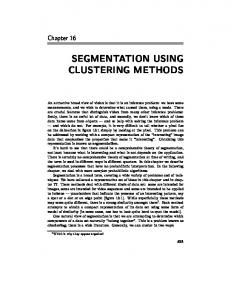
Fig. 1: Overview of our fully automatic two-step multi-label segmentation pipeline. The first CNN uses a low resolution volume as input to localize the center of the bounding box around all heart substructures. The second CNN crops a region around this center and performs the multi-label segmentation.
In this work, we propose a deep learning framework for fully automatic multilabel segmentation of volumetric images. The first convolutional neural network (CNN) localizes the center of the bounding box around all heart substructures. Based on this bounding box, the second CNN predicts the label positions, i.e., the spatial region each label occupies in the volume. By transforming intermediate label predictions to positions of other labels, this second CNN learns the relative positions among labels and focuses on anatomically feasible positions. We evaluate our proposed method on the MM-WHS challenge dataset consisting of CT and MRI volumes.
2
Method
We perform fully automatic multi-label whole heart segmentation from CT or MRI data with CNNs using volumetric kernels. Due to the increased memory and runtime requirements when applying such CNNs to 3D data, we use a two-step pipeline that first localizes the heart on lower resolution volumes, followed by obtaining the final segmentation on a higher resolution. This pipeline is illustrated in Fig. 1. Localization CNN: As a first step, we localize the approximate center of the heart. Although different localization strategies could be used for this purpose, e.g., [9], to stay within the same machine learning framework for all steps we perform landmark localization with a U-Net-like fully convolutional CNN [8, 5] using heatmap regression [10, 7, 6], trained to regress the center of the bounding
Multi-Label Segmentation Using Anatomical Label Configurations
3
box around all heart substructure segmentations. Due to memory restrictions, we downsample the input volume and let the network operate on a low resolution. Then, we crop a fixed size region around the predicted bounding box center and resample voxels from the original input volume on a higher resolution than for localizing bounding box centers. We define the fixed size of this region, such that it encloses all segmentation labels on every image from the training set, thus covering all the anatomical variation occurring in the training data. Segmentation CNN: A second CNN for multi-label classification predicts the labels of each voxel inside the cropped region from the localization CNN (see Fig. 1). For this segmentation task, we use an adaptation of the fully convolutional end-to-end trained SpatialConfiguration-Net from [6] that was originally proposed for landmark localization. The main idea in [6] is to learn from relative positions among structures to focus on anatomically feasible configurations as seen in the training data. In a three stage architecture, the network generates accurate intermediate label predictions, transforms these predictions to positions of other labels, and combines them by multiplication. In the first stage, a U-Net-like architecture [8], which has as many outputs as segmentation labels, generates the intermediate label predictions. For each output voxel, a sigmoid activation function is used to restrict the values between 0 and 1, corresponding to a voxel-wise probability prediction of all labels. Then, in the second stage, the network transforms these probabilities to the positions of other labels, thus allowing the network to learn feasible anatomical label configurations by suppressing infeasible intermediate predictions. As the estimated positions of other labels are not precise, for this stage we can downsample the outputs of the U-Net to reduce memory consumption and computation time without losing prediction performance. Consecutive convolution layers transform these downsampled label predictions to the estimated positions of other labels. Upsampling back to the input resolution leads to transformed label predictions, which are entirely based on the intermediate label probabilities of other labels. Finally, in the last stage, multiplying the intermediate predictions from the U-Net with the transformed predictions results in the combined label predictions. For more details on the SpatialConfiguration-Net, we refer the reader to [6]. Without any further postprocessing, choosing the maximum value among the label predictions for each voxel leads to the final multi-label segmentation.
3
Experimental Setup
Dataset: We evaluated the networks on the datasets of the MM-WHS challenge. The organizers provided 20 CT and 20 MRI volumes with corresponding manual segmentations of seven whole heart substructures. The volumes were acquired in clinics with different scanners, resulting in varying image quality, resolution and voxel spacing. The maximum physical size of the input volumes for CT is 300 × 300 × 188 mm3 while for MRI it is 400 × 360 × 400 mm3 . The maximum size of the bounding box around the segmentation labels for CT is 155 × 151 × 160 mm3 (MRI: 180 × 153 × 209 mm3 ).
4
Payer et al.
Implementation Details: We train and test the networks with Caffe [3] where we perform data augmentations using ITK1 , i.e., intensity scale and shift, rotation, translation, scaling and elastic deformations. We apply these augmentations on the fly during network training. We optimize the networks using Adam [4] with learning rate 0.001 and the recommended default parameters from [4]. Due to memory restrictions coming from the volumetric inputs and the use of 3D convolution kernels, we choose a mini-batch size of 1. Hyperparameters for training and network architecture were chosen empirically from the cross validation setup. All experiments were performed on an Intel Core i7-4820K based workstation with a 12 GB NVidia Geforce TitanX. Input Preprocessing: The intensity values of the CT volumes are divided by 2048 and clamped between −1 and 1. For MRI, the intensity normalization factor is different for each image. We divide each intensity value by the median of 10% of the highest intensity values of each image to be robust to outliers. In this way, all voxels are in the range between 0 and 1; we multiply them with 2, shift them by −1, and clamp them between −1 and 1. For random intensity augmentations during training, we shift intensity values by [−0.1, 0.1] and scale them by [0.9, 1.1]. As we know the voxel spacing of each volume, we resample the images trilinearly to have a fixed isotropic voxel spacing for each network. In training, we randomly scale the volumes by [0.8, 1.2] and rotate the volumes by [−10◦ , 10◦ ] in each dimension. We additionally employ elastic deformations by moving points on a regular 8 × 8 × 8 voxel grid randomly by up to 10 voxels, and interpolating with 3rd order B-splines. All random operations sample from a uniform distribution within the specified intervals. During testing, we do not employ any augmentations. Localization CNN: We localize the bounding box centers with a U-Net-like network using heatmap regression. The U-Net has an input voxel size of 32×32× 32 voxels and 4 levels. For the CT images, we resample the input volumes to have an isotropic voxel size of 10 mm3 (MRI: 12 mm3 ), which leads to a maximum input volume size of 320 × 320 × 320 mm3 (MRI: 384 × 384 × 384 mm3 ). Then, we feed the resampled, centered volumes as input to the network. Each level of the contracting path as well as the expanding path consists of two consecutive convolution layers with 3×3×3 kernels and zero padding. Each convolution layer, except the last one, has a ReLU activation function. The next deeper levels with half the resolution are generated with average pooling; the next higher levels with twice the resolution are generated with trilinear upsampling. Starting from 32 outputs at the first level, the number of outputs of each convolution layer at the same level is identical, while it is doubled at the next deeper level. We employ dropout of 0.5 after the convolutions of the contracting path in the deepest two levels. A last convolution layer at the highest level with one output generates the predicted heatmap. The final output of the network is resampled back to the original input volume size with tricubic interpolation, to generate more precise localization. The networks are trained with L2 loss on each voxel to predict a Gaussian target heatmap with σ = 1.5. We initialize the convolution 1
The Insight Segmentation and Registration Toolkit https://www.itk.org/
Multi-Label Segmentation Using Anatomical Label Configurations
5
layer weights with the method from [2], except for the last layer, where we sample from a Gaussian distribution with standard deviation 0.001. All biases are initialized with 0. We train the network for 30000 iterations. Segmentation CNN: The segmentation network is structured as follows. The intermediate label predictions are generated with a similar U-Net as used for the localization, but twice the input voxel size, i.e., 64 × 64 × 64, and twice the number of convolution layer outputs. For the CT images, we resample the input images trilinearly to have an isotropic voxel size of 3 mm3 (MRI: 4 mm3 ), which leads to a maximum input volume size of 192 × 192 × 192 mm3 (MRI: 256×256×256 mm3 ). The final layer of this U-Net generates eight outputs, which correspond to the number of segmentation labels, i.e., seven heart substructures and the background. This layer has a sigmoid activation function to predict intermediate probabilities. Then in the subsequent label transformation stage, the outputs of the previous stage are downsampled with average pooling by a factor of 4 in each dimension. Four consecutive convolution layers with kernel size 5 × 5 × 5 and zero padding transform the downsampled outputs of the U-Net. The intermediate layers have 64 outputs with a ReLU activation function, while the last layer has eight outputs with linear activation. A final trilinear upsampling resizes the output back to the resolution of the first stage. After multiplying the predictions of the U-Net and the label transformation stage, a softmax with multinomial logistic loss on each voxel is used as a target function. The final output of the network is resampled back to the original input volume size with tricubic interpolation, to generate more precise segmentations. The weights of each layer are initialized as proposed in [2]; the biases are initialized with 0. We train the network for 50000 iterations. To show the impact of the label transformation stage on the total performance, we additionally train a U-Net that is identical to the first stage of the segmentation CNN, without the subsequent label transformation.
4
Results and Discussion
To evaluate our proposed approach, we performed a three-fold cross validation on the training images of the MM-WHS challenge for both imaging modalities, such that each image is tested exactly once. Additionally, the organizers of the MM-WHS challenge provided the ranked results of the challenge participants on the undisclosed manual segmentations of the test set. The localization network achieved a mean Euclidean distance to the ground truth bounding box centers of 13.2 mm with 5.4 mm standard deviation for CT, and 20.0 mm ± 30.5 mm for MRI, respectively. Despite the larger standard deviation for MRI, we observed that this is sufficient for the subsequent cropping, i.e., the input for the multi-level segmentation network, as the cropped region encloses the segmentation labels of all heart substructures of all tested images from the training set. We provide evaluation results of our proposed multi-label segmentation CNN and of our implementation of the U-Net. The Dice Similarity Coefficients are
6
Payer et al.
Table 1: Dice Similarity Coefficients in % for the U-Net-like CNN (U-Net) and our proposed segmentation CNN (Seg-CNN). The values show the mean (± standard deviation) of all images from the CT and MRI cross validation setup for each segmentation label. Label abbreviations: LV - left ventricle blood cavity, Myo - myocardium of the left ventricle, RV - right ventricle blood cavity, LA left atrium blood cavity, RA - right atrium blood cavity, aorta - ascending aorta, PA - pulmonary artery, µ - average of the seven whole heart substructures.
CT
U-Net
MRI
Seg-CNN U-Net Seg-CNN
LV Myo RV LA RA aorta PA µ 91.0 86.1 88.8 91.0 86.5 94.0 83.7 88.7 (± 4.3) (± 4.2) (± 3.9) (± 5.2) (± 6.0) (± 6.2) (± 7.7) (± 3.3) 92.4 87.2 87.9 92.4 87.8 91.1 83.3 88.9 (± 3.3) (± 3.9) (± 6.5) (± 3.6) (± 6.5) (± 18.4) (± 9.1) (± 4.3) 81.1 68.1 76.2 74.0 77.0 70.6 68.7 73.7 (± 23.8) (± 25.3) (± 24.9) (± 24.7) (± 22.1) (± 20.2) (± 16.5) (± 21.4) 87.7 75.2 77.7 81.1 82.7 76.6 72.0 79.0 (± 7.7) (± 12.1) (± 19.5) (± 13.8) (± 15.8) (± 13.8) (± 16.1) (± 11.7)
CT
1. 2. 3. 4. 5. 6. 7. 8.
LV 91.8 92.3 90.4 90.1 90.8 89.3 88.0 59.3
Myo 88.1 85.6 85.1 84.6 87.4 83.7 81.5 53.3
RV 90.9 85.7 88.3 85.6 80.6 81.0 84.9 70.6
LA 92.9 93.0 91.6 88.4 90.8 88.9 84.5 72.0
RA 88.8 87.1 83.6 83.7 85.5 81.2 79.9 51.5
aorta 93.3 89.4 90.7 91.4 83.5 86.8 83.9 60.1
PA 84.0 83.5 78.4 80.0 67.7 69.8 73.7 63.7
WHS 90.8 89.0 87.9 87.0 86.6 84.9 83.8 62.3
MRI
Table 2: Dice Similarity Coefficients on the CT and MRI test sets of the MMWHS challenge for all participants in %, ranked by highest score. The values show the mean of all images for each segmentation label. The results of our approach are highlighted in yellow. Label abbreviations: same as Table 1, WHS - whole heart segmentation.
1. 2. 3. 4. 5. 6. 7. 8.
91.8 91.6 87.1 89.7 83.6 85.5 75.0 70.2
78.1 77.8 74.7 76.3 72.1 72.8 65.8 62.3
87.1 86.8 83.0 81.9 80.5 76.0 75.0 68.0
88.6 85.5 81.1 76.5 74.2 83.2 82.6 67.6
87.3 88.1 75.9 80.8 83.2 78.2 85.9 65.4
87.8 83.8 83.9 70.8 82.1 77.1 80.9 59.9
80.4 73.1 71.5 68.5 69.7 57.8 72.6 47.0
87.0 86.3 81.8 81.7 79.7 79.2 78.3 67.4
Multi-Label Segmentation Using Anatomical Label Configurations
(a) Dice: 94.11% (ct train 1001)
(b) Dice: 76.43% (ct train 1019)
(c) Dice: 88.39% (mr train 1017)
(d) Dice: 42.11% (mr train 1001)
7
Fig. 2: Segmentation results of volumes with best and worst Dice scores for CT (top row) and MRI (bottom row) datasets. Volumes on the left show predictions; volumes on the right show corresponding ground truth segmentation.
shown in Table 1, where both approaches perform similar for the CT dataset. However, in the MRI dataset, which shows more variation in anatomical field of view, intensity ranges and acquisition artifacts compared to CT data, the improvements when adding the label configuration stage are very prominent. We assume that the larger variability of MRI data would require more training data for the U-Net, while our proposed label transformation stage compensates the lack of training data by focusing on anatomically feasible configurations. Figure 2 shows qualitative segmentation results of the best and worst cases for CT and MRI datasets, respectively. The wrong labels in the ascending aorta of 2b were caused by acquisition artifacts in the CT volume, whereas a failing intensity value normalization of the MRI volume resulted in wrong segmentations in 2d. For generating the segmentations on the test set, we trained the networks on all training images with the same hyperparameters as used for the cross validation. Table 2 shows the results on the test set of the MM-WHS challenge, ranked for all participants selected for the final comparison. By achieving the first place on the CT dataset and the second place on the MRI dataset, our method was the best in overall ranking. Although in CT the results of our own cross validation and the test images of the challenge are similar, in MRI the results on the test set are better than for the cross validation. We think the reason for this is the larger variability in the MRI dataset, such that increasing the number of training images improves the results more drastically as compared to CT. In
8
Payer et al.
future work we are planning to evaluate our method on datasets coming from different scanners and sites.
5
Conclusion
We have presented a method for fully automatic multi-label segmentation from CT and MRI data, using a pipeline of two fully convolutional networks, performing coarse localization of a bounding box around the heart, followed by multi-label segmentation of the heart substructures. Results on the MICCAI 2017 Multi-Modality Whole Heart Segmentation challenge show top performance of our proposed method among the contesting participants. Achieving the first place in the CT and the second place in the MRI dataset, our method was the best performing in overall ranking.
References 1. Grbic, S., Ionasec, R., Vitanovski, D., Voigt, I., Wang, Y., Georgescu, B., Comaniciu, D.: Complete valvular heart apparatus model from 4D cardiac CT. Medical Image Analysis 16(5), 1003–1014 (2012) 2. He, K., Zhang, X., Ren, S., Sun, J.: Delving Deep into Rectifiers: Surpassing Human-Level Performance on ImageNet Classification. In: Proc. Int. Conf. Comput. Vis. pp. 1026–1034. IEEE (2015) 3. Jia, Y., Shelhamer, E., Donahue, J., Karayev, S., Long, J., Girshick, R., Guadarrama, S., Darrell, T.: Caffe: Convolutional Architecture for Fast Feature Embedding. In: Proc. ACM Int. Conf. Multimed. pp. 675–678. ACM (2014) 4. Kingma, D.P., Ba, J.: Adam: A Method for Stochastic Optimization. Int. Conf. Learn. Represent. CoRR, abs/1412.6980 (2015) 5. Long, J., Shelhamer, E., Darrell, T.: Fully Convolutional Networks for Semantic Segmentation. In: Proc. Comput. Vis. Pattern Recognit. pp. 3431–3440. IEEE (2015) ˇ 6. Payer, C., Stern, D., Bischof, H., Urschler, M.: Regressing Heatmaps for Multiple Landmark Localization Using CNNs. In: Proc. Med. Image Comput. Comput. Interv. pp. 230–238. Springer (2016) 7. Pfister, T., Charles, J., Zisserman, A.: Flowing ConvNets for Human Pose Estimation in Videos. In: Proc. Int. Conf. Comput. Vis. pp. 1913–1921 (2015) 8. Ronneberger, O., Fischer, P., Brox, T.: U-Net: Convolutional Networks for Biomedical Image Segmentation. In: Proc. Med. Image Comput. Comput. Interv., pp. 234–241. Springer (2015) ˇ 9. Stern, D., Ebner, T., Urschler, M.: From Local to Global Random Regression Forests: Exploring Anatomical Landmark Localization. In: Proc. Med. Image Comput. Comput. Interv. pp. 221–229. Springer (2016) 10. Tompson, J., Jain, A., LeCun, Y., Bregler, C.: Joint Training of a Convolutional Network and a Graphical Model for Human Pose Estimation. In: Proc. Neural Inf. Process. Syst. pp. 1799–1807 (2014) 11. Zhuang, X., Rhode, K., Razavi, R., Hawkes, D.J., Ourselin, S.: A RegistrationBased Propagation Framework for Automatic Whole Heart Segmentation of Cardiac MRI. IEEE Transactions on Medical Imaging 29(9), 1612–1625 (2010) 12. Zhuang, X., Shen, J.: Multi-scale patch and multi-modality atlases for whole heart segmentation of MRI. Medical Image Analysis 31, 77–87 (2016)