Multi-modal Mapping and Localization of Unmanned Aerial Robots

Multi-modal Mapping and Localization of Unmanned Aerial Robots based on Ultra-Wideband and RGB-D sensing* F.J. Perez-Grau1 , F. Caballero2 , L. Merino3 and A. Viguria1 Abstract— This paper presents a methodology for mapping and localization of Unmanned Aerial Vehicles (UAVs) based on the integration of sensors from different modalities. Particularly, we integrate distance estimations to Ultra-Wideband (UWB) sensors and 3D point-clouds from RGB-D sensors. First, a novel approach for environment mapping is introduced, exploiting the synergies between UWB sensors and point-clouds to produce a multi-modal 3D map that integrates the estimated UWB sensors position. This map is further integrated into a Monte Carlo Localization method to robustly estimate the UAV pose. Finally, the full approach is tested with real indoor flights and validated with a motion tracking system.

I. INTRODUCTION Unmanned Aerial Vehicles (UAVs) have attracted great interest in recent years as a viable, low-cost technology for performing tasks in indoor environments in the context of several applications such as surveillance, inspection or mapping. These applications usually demand precise UAV self-localization in the environment, which is also needed for achieving a safe performance during the flight. Outdoor positioning has greatly benefited from the use of Global Positioning System (GPS) coupled with inertial measurements [1]. However, GPS-based localization is impractical indoors due to the high attenuation of satellite signals. Therefore, alternative technologies have been proposed and developed in the past years in order to achieve robust indoor positioning for UAV applications. Motion capture systems are one of the most common methods for indoor positioning. They are based on visual markers and a network of cameras strategically positioned in order to have overlapping fields of view in the operating area. Several testbeds for UAV robotics research are based on such systems, like Vicon1 [2] [3] , or OptiTrack2 [4] [5]. Nevertheless, these solutions are not cost-effective for scaling to larger or other indoor scenarios, and the line of sight requirement of such systems is difficult to meet in cluttered environments, such as in manufacturing plants. Furthermore, in order to achieve a robust and scalable UAV localization *The work of F.C. and L.M. was partially supported by MINECO (Spain) grant OCELLIMAV (TEC-61708-EXP) 1 F.J. Perez-Grau and A. Viguria are with the Center for Advanced Aerospace Technologies (CATEC), Aerospace Technology Park of Andalusia, 41309 La Rinconada, Sevilla (Spain). Email:

[fjperez,aviguria] at catec.aero 2 F. Caballero is with the Department of Systems Engineering and Automation, University of Seville, Spain. Email: fcaballero at

us.es 3 L. Merino is with School of Engineering, Universidad Pablo de Olavide, Seville, Spain. Email: lmercab at upo.es 1 https://www.vicon.com/ 2 http://www.optitrack.com/

solution, it seems reasonable to compute the pose estimations on-board the aerial robot, unlike the aforementioned offboard motion capture systems. Due to the availability of low-energy sensors and radio frequency circuitry, there is a research trend on radiobased localization systems [6], [7]. This technology uses the received signal to estimate the position of the receiver with respect to fixed emitters. The use of WLAN access points effectively exploits the existing infrastructure in place, making it an easier solution to adopt. However, it does not provide enough accuracy to achieve safe autonomous operation of UAVs [8]. Ultra-Wideband (UWB) is a wireless communication technology which has attracted interest as a promising solution for precise target localization and tracking [9], [10], [11]. It is particularly well suited for short-distance indoor applications, where the position of the on-board sensor can be obtained with an accuracy of a few centimeters. However, estimations can suffer from attenuation across materials, interference from other wireless devices and multipath propagation. As motion capture systems, this solution needs an associated infrastructure to be installed in the environment and properly calibrated. Besides, these sensors are poorly suited to constitute a full localization system due to the lack of bearing information. Other approaches do not rely on existing infrastructure, but on the successful detection of features in the environment by on-board sensors. Probably the most extended approaches for UAVs are based on cameras, due to the amount of provided information versus their low weight. Algorithms for UAV pose estimation based on visual odometry or Simultaneous Localization And Mapping (SLAM) have been widely considered, either using monocular cameras [12], [13] or stereo-vision [14], [15], and more recently RGB-D sensors [16], [17]. The latter solution exhibits an important advantage since its performance does not depend on the scene texture in order to estimate the depth, and is less reliant on lighting conditions while indoors. Visual odometry approaches demonstrate good results in the short term, but are not reliable in the long term due to cumulative drift. SLAM approaches work very well when we repeatedly visit the same area, but usually fail at high-speed UAV motions in unknown scenarios. The computational complexity of these approaches is also an important issue regarding usability and robustness, given the common on-board restrictions in UAVs. Another family of localization techniques are based on maps of the environment, exploiting the fact that UAVs often operate in partially known scenarios. Sensor data can be matched with the map in order to determine the UAV

pose. One of the most common map representations are occupancy grids, introduced several decades ago [18]. An important drawback of these grids is their large memory requirement, but recent developments such as OctoMap [19] provide efficient data structures particularly suited for robotics applications in the constrained equipment usually present on-board UAVs [20], [21]. Monte Carlo Localization (MCL) is one of the most popular approaches that makes use of a known map of the environment, typically in the form of occupancy grids, and is commonly used for robot navigation in indoor environments [22], [23]. However, most MCL approaches are meant for wheeled robots moving in 2D environments, requiring a 2D laser scanner for map building and localization. Other authors presented an extension for 6D localization based on 2D laser scanner [24], but it is meant for 2D motion of humanoid robots in a 3D environment, which makes it not suitable for aerial robots. II. M APPING AND LOCALIZATION APPROACH The aforementioned approaches are promising in that they can all provide solutions to the localization problem, but important drawbacks are present using each of them alone. Infrastructure-based positioning systems achieve reliable performances, but they can be expensive and might require laborious setup and calibration processes. Visionbased approaches demonstrate good results relying only on on-board equipment, but are not robust when applied to UAVs. Map-based methods are robust solutions for longterm localization, but often demand a high computational cost apart from the need to previously build an accurate representation of the environment. The main contribution of this work focuses on the combination of technologies in order to achieve long-term autonomous operation of UAVs in indoor environments, taking advantage of their respective benefits to overcome their main drawbacks. In particular, a visual odometry algorithm based on an RGB-D camera adapted from [25] and a localization algorithm based on UWB sensors have been merged into a MCL algorithm that relies on a previously built multi-modal map, which includes 3D data and UWB sensors location. The different technologies benefit from each other: • The visual odometry provides a reliable short-term pose estimation, while its drift is bounded thanks to the map matching and UWB measurements. • The noise and outliers from the UWB sensors are filtered thanks to the odometry prior. • The MCL exploits the visual odometry to update the motion of the particles, and the UWB measurements to maintain a low dispersion on the position of the particles whenever the map matching is not acceptable. This solution offers reliable localization in position and yaw angle, while roll and pitch angles can still be observable through an IMU. Moreover, the implemented algorithms are highly efficient so they are suitable for real-time operation on-board the aerial robot for performing on-line localization. The rest of the paper is structured as follows. The multimodal map building process is detailed in Section III. This

map is used together with RGB-D and UWB data into the MCL approach described in Section IV to perform UAV localization. Finally, experimental results are presented in Section V, followed by conclusions and future work. III. M ULTI - MODAL MAPPING WITH UAV S As previously introduced, prior to robot localization, this approach will map the environment. The objective is to jointly estimate the position of a set of fixed UWB sensors (beacons) and also to 3D map the environment in the same reference frame based on RGB-D data. One possible approach is to solve these two problems separately. That is, mapping the scene and accurately localizing the robot based on local sensors, and later on, using this information to map the position of the UWB sensors into the environment. However, this approach does not take advantage of the UWB sensors for mapping, neither for localization. This paper follows an integrated approach in which the positions of the UWB sensors are firstly approximated and later on refined together with the 3D map of the environment. This way, the first step will consider the range information from the UWB alone to compute a globally consistent robot trajectory in 3D and to automatically detect loop-closures without human intervention. Then both, the computed trajectory and the loop-closures, will be used in a second step to optimize the position of the robot in 3D and also the UWB sensors position. Next paragraphs will give further details of both steps. A. Step 1: Range-only localization and mapping The objective of this step is to compute an initial guess of the UWB sensors’ positions, based on distance measurements from the sensors to the robot, and to use this information to obtain a globally consistent trajectory of the UAV. This is generally referred a Range-Only Simultaneous Localization and Mapping (or RO-SLAM) Most of the approaches for RO-SLAM in the state of the art are based on time filtering and probabilistic frameworks as EKF-SLAM, UKF-SLAM, FatSLAM and others [26], [27]. In [26] it is shown how the unscented FastSLAM presents better results over other classical methods based on EKF or UKF. However, FastSLAM solutions do not preserve the correlation between different landmarks of the map in those applications in which it might exist. Other landmarkbased SLAM algorithm is considered in [28], where the authors use a particle filter to initialize the EKF filter for each new landmark. The main drawback of the previous approaches lies in the delayed initialization of the landmarks into the filters which significantly reduces the optimization of the robot localization until the solution position of the range sensors have converged. This problem is solved in [29] where a batch solution is proposed to estimate the mobile robot and landmarks position using a singular value decomposition (SVD) of the observation matrix. A batch processing solution is also presented in [30] based on optimization. However, these methods assume

measurements from all the UWB sensors at every robot position, otherwise the measurement must be interpolated. This is a hard constraint in realistic implementations where the visibility of all the UWB sensors cannot be guaranteed all the time. This paper proposes a new optimization approach for the RO-SLAM problem that follows the batch processing ideas but generalizes to a more common situation in which the range measurements from the UWB sensors might arrive at the robot independently, even having robot poses without related range measurements. 1) Problem definition: We denote a robot trajectory with N poses as X = {x1 , x2 , ..., xN } and the positions of a set of M UWB range sensors as B = {b1 , b2 , ..., bM }, where each robot pose is represented as xi = [xi , yi , zi , ψi ]T and the UWB sensor position as bj = [bxj , byj , bzj ]T . Given a set of observations D = {dij }, where each dij is the Euclidean distance between the position corresponding to pose xi (defined as xpi = [xi , yi , zi ]T ) and sensor position bj , the objective of the RO-SLAM optimization problem is to compute the robot trajectory X and UWB sensors positions B that best fit the measured distances. Notice how the robot roll and pitch angles are not included into the robot pose definition. We assume these angles are available and accurate enough in an UAV. They are fully observable and they are usually accurately computed in aerial robots because they are the most basic control variables (together with the rotation rates) for the system stability. While it is true that roll and pitch estimation based on accelerometer and gyroscope integration might be biased under constant acceleration (like loitering in fixedwing UAVs), these scenarios are very rare to occur indoors. In addition, we will assume we can estimate the bz parameter of every UWB sensor position in B by just measuring the distance to the floor. This is an easy process that can be implemented accurately. This assumption allows reducing the number of unknown parameters of the UWB sensor position to two, but we still do not have enough information to initialize the UWB sensor position into the optimization. We model the observations at pose xi as the set of measurements zi = {di1 , di2 , ..., diM } with arbitrary length from 0 (no measurements) to M (measurements to all UWB sensors). Thus, the resultant robot trajectory and UWB sensors positions will be the ones that minimize the following expression:   N X M X arg min  cij (kxpi − bj k−dij )2  (1) {X,B}

i=1 j=1

where cij is a variable that takes value 1 if there is a measurement from pose xi to UWB sensor bj and 0 otherwise. However, due to the nature of the problem addressed, there exists the possibility that a number of poses have not measurements at all (the robot is out of range of all UWB sensors) and, more frequently, that the number of range

Fig. 1. Multiple hypotheses for the localization of three UWB sensors. The robot performs a 3D trajectory, but it is shown an orthogonal view for easy visualization of the position hypotheses. Triangles are robot poses and circles are UWB sensor position hypotheses

measurements in a pose is below four (minimum number of range measurements to compute the robot position in 3D). These limitations are overcome by including the odometric constraints into Eqn. (1), obtaining the final expression to minimize:    N M X X E(xi , xi−1 ) + cij (kxpi − bj k−dij )2  arg min  {X,B}

i=1

j=1

(2) where E(...) stands for the squared error function between pose xi and xi−1 according to the odometry information. This function transforms the pose xi−1 according to the odometry and computes the error with respect xi in each pose dimension. We make use of the stereo-vision odometry algorithm presented by the authors in [25] (which is publicly available3 ), adapted to the particularities of RGB-D sensors. 2) Optimization: Solving Eqn. (2) is straightforward if we have an good initial guess about the robot poses and the UWB sensor positions. However, in RO-SLAM we have no information about the position of the range sensors. We can of course initialize B to random positions and let the optimization process to estimate the correct ones, but the optimizer will be stack in a local minimum almost for sure. Instead, we re-parameterize the UWB sensor position so that we can have several hypotheses of the estimation into the optimizer as done in [31]. Thus, when the robot at pose xi receives the first range measurement dij to sensor j, we know the sensor is in circle at altitude bzj around the current robot pose (see Fig. 1 as example). This paper proposes sampling this circle with multiple position hypotheses and letting the optimizer to choose the better one. Thus, assuming Hj different hypotheses for sensor j, the UWB sensor position will be parametrized as follows: bj = [bj1 , bj2 , ..., bjHj ] 3 http://wiki.ros.org/viodom

(3)

where each single position hypothesis is represented as bjk = [bxjk , byjk , bzj ]t . Notice how bzj is the same for all hypotheses because it is actually a known parameter. With this parameterization in mind, we can reformulate Eqn. (2) as follows:   N X E(xi , xi−1 ) arg min  {X,B}

i=1

 Hj M X X 1 + cij (kxpi − bjk k−dij )2  H j j=1

(4)

To this end, we transform each point-cloud to the global reference frame according to its associated pose (pcgi ) and compute the alignment error between point-clouds as the averaged Euclidean distance between their individual 3D points. Then, Eqn. (2) (because now we have a single hypotheses for each UWB position) can be enlarged with this new constraint as follows:   N X E(xi , xi−1 ) arg min  (8) {X,B}

k=1

+

Notice how the contribution of a single UWB sensor j is scaled by 1/Hj for every pose xi so that we do not double-count the information provided by a single range measurement. 3) Initialization: In summary, the parameters of the optimization process are the position of the robot in each pose xi , which are initialized according to the odometry values, and the different position hypotheses for every UWB sensor. When we receive a range measurement dij from UWB sensor j for the first time, we use the current robot position estimate xi to initialize the Hj position hypotheses according to the following equations:

M X

i=1

cij (kxpi

− bj k−dij )2 +

j=1

Pi X

 D(pcgi , pcgl )

l=1

D(pcgi , pcgl )

byjk

=

yi + dij sin(2π(k − 1)/Hj )

(6)

computes the squared avwhere the function erage distance between the given point-clouds in the global frame and Pi is the number of loop-closures that affect pose i. The computation of D(pcgi , pcgl ) could have a significant computational cost if the involved point-clouds are large because it needs to compute the match between the 3D points of both clouds each time, slowing down the optimization process. However, assuming the poses to be optimized are not far from the final estimates thanks to the RO-SLAM step, we can pre-compute the 3D point data association step between point-clouds. This way, function D(pcgi , pcgl ) only needs to recompute the average distance between 3D points because the association is known.

bzjk

=

bzj

(7)

IV. M AP - BASED L OCALIZATION

bxjk

=

xi + dij cos(2π(k − 1)/Hj )

(5)

for k = 1, . . . , Hj . The value of Hj is initialized to Hj = 10dij , so that the number of hypotheses adapts to the sensor distance. B. Step 2: 3D Mapping and pose refinement The outcome of Step 1 will be a globally consistent trajectory and an initial estimation of the UWB sensors positions. If the robot motion is rich enough to let the optimizer disambiguate the horizontal flip ambiguity [32], then it will converge to a single solution and all the hypotheses will be localized in one position. Now that we have good guess about the UWB sensor positions and also a coherent trajectory, we can perform automatic loop-closing detection on the RGB-D data based on different approaches as visual place recognition or scan matching. This paper implements a massive scan-matching process among all the poses that fall within a given search radius. Given the sensor point-cloud pci at pose xi and the pointcloud pcj and pose xj in a closed-loop, the scan-matching process establishes the transform that best aligns both pointclouds. In the literature, this transform is typically used as a constraint between both poses and its associated information matrix allows tuning the importance of the such constraint into the nonlinear optimization process [33]. Instead, we propose to include the alignment error into the optimization process, as we aim to build an accurate 3D map.

As previously introduced in Section I, we present a MCL method for 6D localization that integrates visual odometry from an RGB-D camera, 3D point clouds from such camera, distance measurements to several UWB sensors installed in the environment, and the 3D map which was built using the approach described in Section III. The particle filter consists of N particles pi , each of them with the following state vector: pi = [x, y, z, ψ]T (9) where ψ refers to the yaw angle of the UAV. Even though a 4D state vector is used, we are able to provide 6D localization estimations since roll and pitch angles are observable through the on-board PNIMU. Each particle has an associated weight wi such as i=1 wi = 1. We assume that the initial state of the robot pose is known, which is usually the case since UAVs often take off from a designated location. We use a motion model to propagate the current state of all the particles according to the visual odometry estimation computed from RGB-D data (we use the same odometry algorithm as in Section III). The state of the particles will evolve according to the following expressions: xt+1 i

=

xti + ∆x ∗ cos(ψit ) − ∆y ∗ sin(ψit ) (10)

yit+1

=

yit + ∆x ∗ sin(ψit ) + ∆y ∗ cos(ψit )

(11)

=

zit + ∆z ψit + ∆ψ

(12)

zit+1 ψit+1

=

(13)

The increments ∆x, ∆y, ∆z and ∆ψ provided by the visual odometry are drawn randomly with standard deviations proportional to each increment itself. A filter update is launched when the translation or rotation thresholds are accomplished. Then, we make use of the latest 3D point clouds from the RGB-D camera and distance measurements to the UWB sensors to update the filter. Each particle pi evaluates its accuracy by checking how likely it would receive such sensor reading at its current pose, thus computing a new weight value wi that is influenced by the two sensors readings (RGB-D and UWB). Thus, the point clouds are transformed to each particle pose in order to find correspondences against the map. Since this is computationally costly, we use a static 3D probability grid in which each cell indicates its probability of being an occupied point of the map. Such probability grid only needs to be computed once, relieving extensive distance computations for each particle, since each point from the 3D point cloud must be evaluated. The particle weight associated to the map matching is calculated as follows: wimap =

M 1 X grid(pi (ck )) M

(14)

k=1

where M is the number of 3D points ck that conform the RGB-D point cloud, pi (ck ) is the point transformed according to the particle state and grid(pi (ck )) is the value of the probability grid in such transformed position. Assuming each 3D point in the cloud isQindependent, we can also compute M this weight as wimap = k=1 grid(pi (ck )), however we opt for the weight average of (14) to avoid numerical errors. On the other hand, distance measurements between UWB sensors are used to compute another weight value for each particle according to how well their state fits to the distribution of fixed radio beacons. The measured radio-based distance dij from the UAV to the j-th beacon is compared to the actual Euclidean distance between pi and bj . The product is used to aggregate the values from the measurements of different beacons, since they are conditionally independent probabilistic processes. The weight value from range sensing wirange is calculated feeding this difference dij − kpi − bj k in a Gaussian probability distribution with zero mean and the UWB sensor standard deviation. In order to combine the weights of both sensing approaches (map and range), all the weights must first be normalized within their categories. This prevents merging values which usually are in different orders of magnitude. A weighted average is used to obtain the final weight of each particle such that wi = α ∗ wimap + (1 − α) ∗ wirange

(15)

Although both sensor measurements are conditionally independent and the weight product is the adequate way to perform the update, we choose the approach in (15) to better deal with the outliers commonly present in indoor UWB sensors. If an outlier in the distance measurement from a UWB sensor is received, this would result in very low values

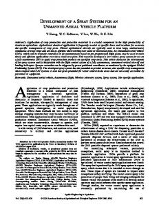
Fig. 2. The UAV with the two RGB-D sensors (Orbbec Astra), left image shows the front view and right image the rear view. The UWB sensor is placed on top of the aerial robot. The passive markers are used by the motion capture system to acquire ground truth data.

for wirange ; in this case the resampling would only depend on the associated weights calculated from the point cloud matching, and the relative scoring among the set of particles would remain unaffected. The next step of the algorithm involves a redistribution of the particles to new poses that are more likely to be accurate, according to their weight. The algorithm employed for resampling is the low variance sampler [34]. The updated state vector for the aerial robot is then calculated as the weighted sum of all the particles. V. E XPERIMENTAL R ESULTS An experimental setup has been conceived in order to test the proposed approach. An UAV has been equipped with two RGB-D sensors, one in the front and another one in the rear side of the robot, as depicted in Fig. 2. An UWB sensor has been also installed into the robot and a set of three UWB sensors have been placed in the scenario. The UWB distance measurements have a standard deviation of 20cm approximately, but they are subject to further distortions due to reflexions or sigma attenuation. The experiments have been carried out in CATEC’s Testbed, a flying arena with dimensions 15x15x5 m equipped with a motion tracking system able to estimate positions with sub-millimeter accuracy. Thus, we can obtain the ground truth of the robot position and also the position of the UWB sensors in the scene. Two different flights were recorded. The UAV first flown in the area to gather sensor information with the purpose of building a map of the environment. Later on, a new flight was done to gather ground-truth information so that we can compare the motion tracking localization with our MCL localization using the previously computed map. The following paragraphs detail each of the experiments. A. Map building With the data gathered in the mapping flight, a pose graph was built and the multiple hypotheses for the three unknown UWB sensors. As previously introduced, we measured the heights bzj of each of the M UWB sensors with respect the ground, so that we only needed to estimate the bxj and byj position of the sensors. The graph build based on the odometric information was optimized to obtain a globally coherent robot localization and also to have a good guess about the UWB sensor localization. The solution of the optimization process is shown in Fig. 3

Fig. 3. Results of the Step 1 optimization. We can see how the total RMS error in position is below 0.3m and 0.18rad in yaw. The errors per axis are presented (red) and the RMS error (blue)

Fig. 5. Top view of the map reconstruction using the point-cloud associated to each robot pose. (Top) Reconstruction using the motion tracking groundtruth for the robot poses. (Bottom) Reconstruction based on the results of the optimization

B. Map-based localization

Fig. 4. Results of the Step 2 optimization. We can see how the total RMS error in position is below 0.16m and 0.04rad in yaw. The errors per axis are presented (red) and the RMS error (blue)

where the error for each of the robot poses is shown. We can see how the error in the robot trajectory is reduced to less than 0.5m in position. The three UWB converged to a single solution with an RMS error of 1.1m. Although this is a significant error, they helped the optimizer to compute a globally consistent robot trajectory, improving the close-loop detection for Step 2. Finally, Fig. 4 shows the results after Step 2 optimization. We are able to reduce the localization error to 0.16m RMS in total, while yaw error is reduced to 0.04rad. In addition, the localization error of the UWB sensors is reduced down to 0.4m RMS, in the order of the sensor noise. Once the full robot trajectory was optimized, the 3D pointclouds from each pose can be projected into a single map to reconstruct the robot environment. Fig. 5 shows the map obtained using the proposed optimization approach and the map computed using the ground-truth poses from the motion tracking system. It can be seen that there are some errors due to inaccuracies in the trajectory, but the the general structure and details are captured in the reconstruction.

The second flight took place with the same scenario layout in order to use the previously built map for localization. Fig. 6 shows the estimated position and yaw angle provided by our MCL method during this flight, along with the groundtruth values provided by the motion capture system. Roll and pitch angles were acquired directly from the on-board IMU and hence are not shown in the plots, since they are directly integrated in the algorithm. The results of this experiment have been included into a video, which can be accessed at the URL https://grvc.us.es/staff/caba/share/iros2017.avi. As it can be seen, the estimations closely follow the ground-truth during all the experiment, and do not exhibit drift with time while keeping the errors approximately bounded. Consistent errors of less than 0.2m were obtained for x and y during the whole trajectory. Errors in z were a bit higher but this could be solved through the use of a lowweight altimeter for robust estimations integrated into the MCL. RMS errors in ψ of 0.07 radians (around 4◦ ), with peaks up to 0.26 radians (15◦ ), are considered acceptable. It is also worth to mention that the UAV traversed not mapped areas during the experiment. The use of UWB sensors greatly helped when the UAV visited previously unexplored regions, or with different yaw angles that led to unknown viewpoints, such as depicted in Fig. 7. In contrast, the map matching allowed a better estimation in z since the radio anchors did not exhibit much difference in height (due to practical reasons in the installation), and especially in ψ since this angle cannot be estimated from the radio sensors

x (m)

x error (m)

Ground Truth Our approach

2 0 -2 -4 0

50

100

150

200

α = 0.5 α=1 α=0

1.5 1 0.5 0 0

250

50

100

y error (m)

y (m)

5 0 -5 50

100

150

200

2 0 100

150

200

250

4 2 0 -2

yaw error (rad)

50

time (s) yaw (rad)

50

100

50

100

150

200

250

200

250

200

250

1

0 50

100

150

time (s) 0.5

0 0

50

100

-4 0

150

0.5 0

0

200

0

time (s) z error (m)

z (m)

4

250

1

250

time (s)

200

0.5 0

0

150

time (s)

time (s)

150

time (s)

250

time (s)

Fig. 6. Estimated UAV position and yaw angle. (Red line) Ground truth data from the motion capture system. (Green line) Localization estimations from our approach.

Fig. 8. Estimated UAV position and yaw angle. Left plots show the comparison between the UAV ground-truth (red line) and the estimations from our approach (green line). Right plots include the errors when comparing with the ground-truth (red line) and the overall RMS error for each axis (blue line). TABLE I RMS L OCALIZATION E RRORS

α=1 α=0 α = 0.5

Only map Only range Combined

x (m) 0.34 0.20 0.16

y (m) 0.38 0.17 0.15

z (m) 0.46 0.24 0.22

ψ (rad) 0.13 0.18 0.07

VI. C ONCLUSIONS AND FUTURE WORK Fig. 7. Distribution of particles (red arrows) around the ground-truth UAV pose (green arrow), showing a moment of the flight in which the RGB-D point cloud barely matched the existing 3D locations of the map in which the MCL relied for localization.

measurements. In order to quantify the contribution of each sensor modality, we have analyzed the same flight data modifying the contribution of map matching and UWB sensors into the MCL in Eqn. (15). Fig. 8 presents a comparison of the errors between ground truth and the estimations of our approach using different values of α. Table I summarizes the RMS errors in position and yaw angle for the experiment flight. As expected, x and y positioning is better when using UWB sensors, while ψ estimations are stronger from the map matching. In this case z values exhibit a significant error in the map matching because as explained before, there were many areas without occupancy data and the particles weighting did not show major differences in order to resample them accordingly. Table I summarizes the RMS errors in position and yaw angle for the experiment flight. It can be seen how the proposed combined approach improves the range-only and the map-only MCL implementations.

This paper presented an approach for multi-modal environment mapping using an UAV, and a localization system that integrates such map and the sensor readings from UWB beacons and RGB-D cameras to build a robust approach. The mapping algorithm exploits the synergies between UWB and RGB-D to build an accurate 3D map of the environment and to localize the UWB sensors into such map. Thus, the proposed optimization scheme allows using the range measurements to the UWB sensors to build a globally consistent robot trajectory that helps to detect loop closures in order to refine the trajectory based on optimization from point-cloud alignment. The localization approach successfully integrates both sensor types to overcome the limitations of each sensor modality by its own. The approach has been tested with two UAV flights, one for mapping and another one for localization, and validated using a motion capture system as UAV position and orientation ground-truth. Future work will consider the integration of other modalities such as visual place recognition. In addition, optimization approaches will also be considered for map-based localization of UAVs in order to increase the estimation accuracy. R EFERENCES [1] M. George and S. Sukkarieh, “Tightly coupled INS/GPS with bias estimation for UAV applications,” in Proceedings of Australiasian

Conference on Robotics and Automation (ACRA), 2005. [2] N. Michael, D. Mellinger, Q. Lindsey, and V. Kumar, “The GRASP Multiple Micro-UAV Testbed,” IEEE Robotics & Automation Magazine, vol. 17, no. 3, pp. 56–65, 2010. [3] S. Lupashin, M. Hehn, M. W. Mueller, A. P. Schoellig, M. Sherback, and R. DAndrea, “A platform for aerial robotics research and demonstration: The flying machine arena,” Mechatronics, vol. 24, no. 1, pp. 41–54, 2014. [4] M. Orsag, C. Korpela, and P. Oh, “Modeling and control of mm-uav: Mobile manipulating unmanned aerial vehicle,” Journal of Intelligent & Robotic Systems, pp. 1–14, 2013. [5] L. Marconi, F. Basile, G. Caprari, R. Carloni, P. Chiacchio, C. Hurzeler, V. Lippiello, R. Naldi, J. Nikolic, B. Siciliano, et al., “Aerial service robotics: The AIRobots perspective,” in Applied Robotics for the Power Industry (CARPI), 2012 2nd International Conference on. IEEE, 2012, pp. 64–69. [6] Y. Gu, A. Lo, and I. Niemegeers, “A survey of indoor positioning systems for wireless personal networks,” IEEE Communications surveys & tutorials, vol. 11, no. 1, pp. 13–32, 2009. [7] R. Mautz and S. Tilch, “Survey of optical indoor positioning systems,” in Indoor Positioning and Indoor Navigation (IPIN), 2011 International Conference on. IEEE, 2011, pp. 1–7. [8] A. Khalajmehrabadi, N. Gatsis, and D. Akopian, “Modern wlan fingerprinting indoor positioning methods and deployment challenges,” arXiv preprint arXiv:1610.05424, 2016. [9] J. Gonz´alez, J.-L. Blanco, C. Galindo, A. Ortiz-de Galisteo, J.-A. Fernandez-Madrigal, F. A. Moreno, and J. L. Mart´ınez, “Mobile robot localization based on ultra-wide-band ranging: A particle filter approach,” Robotics and autonomous systems, vol. 57, no. 5, pp. 496– 507, 2009. [10] J. Tiemann, F. Schweikowski, and C. Wietfeld, “Design of an UWB indoor-positioning system for UAV navigation in GNSS-denied environments,” in Indoor Positioning and Indoor Navigation (IPIN), 2015 International Conference on. IEEE, 2015, pp. 1–7. [11] K. Guo, Z. Qiu, C. Miao, A. H. Zaini, C.-L. Chen, W. Meng, and L. Xie, “Ultra-wideband-based localization for quadcopter navigation,” Unmanned Systems, vol. 4, no. 01, pp. 23–34, 2016. [12] A. Davison, I. Reid, N. Molton, and O. Stasse, “MonoSLAM: RealTime Single Camera SLAM,” Pattern Analysis and Machine Intelligence, IEEE Transactions on, vol. 29, no. 6, pp. 1052–1067, June 2007. [13] S. Weiss, D. Scaramuzza, and R. Siegwart, “Monocular-SLAMbased navigation for autonomous micro helicopters in GPS-denied environments,” Journal of Field Robotics, vol. 28, no. 6, pp. 854–874, 2011. [Online]. Available: http://dx.doi.org/10.1002/rob.20412 [14] A. Geiger, J. Ziegler, and C. Stiller, “StereoScan: Dense 3D Reconstruction in Real-Time,” in Intelligent Vehicles Symposium (IV), 2011 IEEE, June 2011, pp. 963–968. [15] K. Schmid, T. Tomic, F. Ruess, H. Hirschmller, and M. Suppa, “Stereo vision based indoor/outdoor navigation for flying robots,” in 2013 IEEE/RSJ International Conference on Intelligent Robots and Systems, Nov 2013, pp. 3955–3962. [16] F. Endres, J. Hess, N. Engelhard, J. Sturm, D. Cremers, and W. Burgard, “An Evaluation of the RGB-D SLAM System,” in Robotics and Automation (ICRA), 2012 IEEE International Conference on, May 2012, pp. 1691–1696. [17] C. Kerl, J. Sturm, and D. Cremers, “Robust odometry estimation for RGB-D cameras,” in Robotics and Automation (ICRA), 2013 IEEE International Conference on. IEEE, 2013, pp. 3748–3754. [18] H. Moravec and A. Elfes, “High resolution maps from wide angle

[19]

[20] [21]

[22] [23]

[24]

[25]

[26]

[27]

[28]

[29] [30] [31]

[32]

[33] [34]

sonar,” in Robotics and Automation. Proceedings. 1985 IEEE International Conference on, vol. 2. IEEE, 1985, pp. 116–121. A. Hornung, K. M. Wurm, M. Bennewitz, C. Stachniss, and W. Burgard, “OctoMap: An efficient probabilistic 3D mapping framework based on octrees,” Autonomous Robots, vol. 34, no. 3, pp. 189–206, 2013. D. Droeschel, M. Nieuwenhuisen, M. Beul, D. Holz, J. St¨uckler, and S. Behnke, “Multilayered mapping and navigation for autonomous micro aerial vehicles,” Journal of Field Robotics, 2015. M. Nieuwenhuisen, D. Droeschel, M. Beul, and S. Behnke, “Obstacle detection and navigation planning for autonomous micro aerial vehicles,” in Unmanned Aircraft Systems (ICUAS), 2014 International Conference on. IEEE, 2014, pp. 1040–1047. S. Thrun, D. Fox, W. Burgard, and F. Dellaert, “Robust Monte Carlo localization for mobile robots,” Artificial intelligence, vol. 128, no. 1-2, pp. 99–141, 2001. M. Quigley, K. Conley, B. Gerkey, J. Faust, T. Foote, J. Leibs, R. Wheeler, and A. Y. Ng, “ROS: an open-source Robot Operating System,” in ICRA workshop on open source software, vol. 3, no. 3.2, 2009, p. 5. A. Hornung, K. M. Wurm, and M. Bennewitz, “Humanoid robot localization in complex indoor environments,” in Intelligent Robots and Systems (IROS), 2010 IEEE/RSJ International Conference on. IEEE, 2010, pp. 1690–1695. F. J. Perez-Grau, F. R. Fabresse, F. Caballero, A. Viguria, and A. Ollero, “Long-term aerial robot localization based on visual odometry and radio-based ranging,” in 2016 International Conference on Unmanned Aircraft Systems (ICUAS), June 2016, pp. 608–614. Z. Kurt-Yavuz and S. Yavuz, “A comparison of EKF, UKF, FastSLAM2.0, and UKF-based FastSLAM algorithms,” in 2012 IEEE 16th International Conference on Intelligent Engineering Systems (INES), June 2012, pp. 37 –43. J. Li, L. Cheng, H. Wu, L. Xiong, and D. Wang, “An overview of the simultaneous localization and mapping on mobile robot,” in 2012 Proceedings of International Conference on Modelling, Identification Control (ICMIC), June 2012, pp. 358 –364. D. Hai, Y. Li, H. Zhang, and X. Li, “Simultaneous localization and mapping of robot in wireless sensor network,” in 2010 IEEE International Conference on Intelligent Computing and Intelligent Systems (ICIS), vol. 3, Oct. 2010, pp. 173 –178. B. Boots and G. J. Gordon, “A spectral learning approach to range-only SLAM,” arXiv:1207.2491, July 2012. [Online]. Available: http://arxiv.org/abs/1207.2491 A. Kehagias, J. Djugash, and S. Singh, “Range-only SLAM with interpolated range data,” Carnegie Mellon University, Tech. Rep., 05 2006. F. R. Fabresse, F. Caballero, I. Maza, and A. Ollero, “Undelayed 3d RO-SLAM based on gaussian-mixture and reduced spherical parametrization,” in 2013 IEEE/RSJ International Conference on Intelligent Robots and Systems (IROS), Tokyo Big Sight, Tokyo, Japan, Nov. 2013, pp. 1555–1561. F. Fabresse, F. Caballero, L. Merino, and A. Ollero, “Active perception for 3D Range-only Simultaneous Localization and Mapping with UAVs,” in Proceedings of the International Conference on Unmanned Aircraft Systems, ICUAS, 2016, pp. 1–6. G. Grisetti, R. Kuemmerle, C. Stachniss, and W. Burgard, “A tutorial on graph-based SLAM,” Intelligent Transportation Systems Magazine, IEEE, vol. 2, no. 4, pp. 31–43, 2010. S. Thrun, W. Burgard, and D. Fox, Probabilistic Robotics (Intelligent Robotics and Autonomous Agents). The MIT Press, 2005.