Multi-Point Relaying Techniques with OSPF on Ad Hoc Networks E. Baccelli, J.A. Cordero and P. Jacquet INRIA Saclay, France Contact Email:
[email protected]
Abstract Incorporating multi-hop ad hoc wireless networks in the IP infrastructure is an effort to which a growing community participates. One instance of such activity is the extension of the most widely deployed interior gateway routing protocol on the Internet, OSPF, for operation on MANETs. Such extension allows OSPF to work on heterogeneous networks encompassing both wired and wireless routers, which may self-organize as multi-hop wireless subnetworks, and be mobile. Three solutions have been proposed for this extension, among which two based on techniques derived from multi-point relaying (MPR). This paper analyzes these two approaches and identifies some fundamental discussion items that pertain to adapting OSPF mechanisms to multihop wireless networking, before concluding with a proposal for a unique, merged solution based on this analysis.
1. Introduction At the price of having considerably more complex mechanisms, link state algorithms produce protocols that don’t diverge, that converge faster and that are better at avoiding routing loops, compared with algorithms based on distance vector (the previous dominating technique for interior gateway routing). The most typical examples of link state protocols are OSPF (Open Shortest Path First [1] [2]) and IS-IS (Intermediate System to Intermediate System [17]), the former being the most widely deployed interior gateway routing protocol on the Internet so far. More recently, multi-hop wireless networks, such as Mobile Ad-hoc NETworks (MANETs), wireless sensor networks [18], or wireless mesh networks, are emerging as new and important networking components. Specific routing protocols have thus been designed to work on this new type of network, which presents harsh characteristics such as higher topology change rates, lower bandwidth, lower transmission quality, more security threats, more scalability issues and as well as novel energy and memory constraints aboard smaller mobile network elements. OLSR (Optimized Link State Routing [3]) is the most wellknown routing protocol for multi-hop wireless networks
based on a link state approach, which, incidently, makes it very similar to OSPF. One question then immediately comes to mind: if OSPF and OSLR are so similar, why is OSPF not also used on multi-hop wireless networks? Operating OSPF on this new type of network is indeed a seducing idea for at least two reasons (i) legacy: OSPF is extremely well deployed, known, and renowned, thus facilitating greatly the integration of multi-hop wireless networking, and (ii) seamless unification of wired and wireless IP networking under a single routing solution: an interesting perspective industry-wise, in terms of maintenance, and costs. There are in fact multiple issues with the use of OSPF in ad-hoc networks [20] [19]. The main problem is the amount of overhead necessary for OSPF to function, which is too substantial for the low bandwidth available so far on multi-hop wireless networks. However, OSPF has a modular design, using different modules called interface types, each tailored for specific technologies, such as Ethernet (Broadcast interface type), or Frame Relay (Point-to-Multipoint interface type). An extension of OSPF, namely a new OSPF interface type for multi-hop wireless networks , would thus be desireable. The goal is an extension that adapts well to the characteristics of multi-hop wireless networks, while letting OSPF run unaltered on usual networks and existing interfaces; a must, for obvious reasons including legacy and backward compatibility with networks currently running standard OSPF. The devices targeted by such an extension are assumed to have reasonable CPU, memory, battery and mobility characteristics. In other words, rather Cisco mobile routers aboard vehicles that move at low or medium speeds, than sensor nodes or MANET nodes at high-speed . Several extension proposals have recently emerged [13] [6] [8], along the lines described above. Among these proposals, a category can be identified which relies on the use of multi-point relaying (MPR [3]), a technique developed and used in various ad hoc networking environments over the past decade. The proposals in this category, including [13] and [6], essentially propose different configurations of similar concepts based on MPR (see Fig. 1).
and interferences between neighbors call for a significant reduction of OSPF control traffic [5]. At the same time, router mobility requires Hello and LSA periods to be drastically shortened in order to be able to track topology changes, implying heavier control traffic, without even more efficient control traffic reduction techniques. The standard OSPF mechanism providing control traffic reduction is the designated router mechanism OSPF [1]. However, in a wireless ad hoc environment, this mechanism is not functional, due to the fact that wireless neighbors generally do not have the same set of wireless neighbors [18]. OSPF extensions for MANET thus use alternative mechanisms. Aside of miscellaneous tweaks and tricks such as implicit acknowledgements or control traffic multicasting (instead of unicast), these alternative mechanisms can be classified in the following categories: Figure 1. Multi-Point Relaying. The center node selects sufficient relays (in black), to cover every node two hops away. Selected relays are then called called MPRs. The dashed circle is the radio range of the center node.
•
•
The remainder of this paper thus analyses how these MPR concepts are configurable, then discusses and evaluates the respective merits of each configuration via simulations. For details on the simulation environment, refer to the appendix. The paper concludes by proposing, based on this analysis, a recommended configuration for MPR-based OSPF operation on MANETs.
2. OSPF on Ad Hoc Networks As a proactive link-state routing protocol, OSPF [1] [2] employs periodic exchanges of control messages to accomplish topology discovery and maintenance: Hellos are exchanged locally between neighbors to establish bidirectional links, while LSAs reporting the current state of these links are flooded (i.e. diffused) throughout the entire network. This signalling results in a topology map, the link state database (LSDB), being present in each node in the network, from which a routing table can be constructed. An additional mechanism, particular to OSPF, provides explicit pairwise synchronization of the LSDB between some neighbors, via additional control signalling (database description messages and acknowledgements). Such neighbor pairs are then called adjacent neighbors, while other bidirectional neighbors are called 2-WAY. In a wireless ad hoc environment, limited bandwidth
•
•
Flooding Optimization and Backup. Instead of the usual, naive flooding scheme, use more sophisticated techniques that reduces redundant retransmissions. Adjacency Selection. Instead of attempting to become adjacent with all its neighbors, a router becomes adjacent with only some selected neighbors. Topology Reduction. Report only partial topology information in LSAs, instead of full topology information. Hello Redundancy Reduction. In some Hello messages, report only changes in neighborhood information instead of full neighborhood information.
This paper discusses the respective merits of set of mechanisms or parameters used in each category, i.e. the different configurations, based on the use of MPR techniques which [6] and [13] have in common. The configurations evaluated in the remainder of this paper are summarized in Table 1. Note that hello redundancy reduction mechanisms discussed independently in Section 6.
3. Flooding Optimization In all considered configurations, MPR (see Fig. 1) is used to determine flooding relays and reduce the number of forwarders of a given disseminated packet, while still ensuring that this packet is sent to each router in the network. However, in case no acknowledgement is received, different backup retransmissions policies are employed, depending on the configuration in use:
Flooding Optimization Flooding Backup Adjacency Selection Topology Reduction
Configuration 1 1.1 1.2 MPR Flooding Overlapping Relays Backup Smart Peering Selection Unsynchr. Smart Peering adjacencies Reduction
Configuration 2 2.1 2.2 MPR Flooding Adjacency MPR Backup Backup MPR Adj. SLO-T Selection Selection MPR Topology Reduction
LSA retransmission ratio (20 nodes, 5 m/s) 1.6
1.4
1.2
1
0.8
Table 1. Considered configurations.
0.6
0.4
•
•
•
Backup per adjacency. A router receiving an LSA from an adjacent neighbor must acknowledge its reception to the neighbor. Absent this acknowledgement, the neighbor must retransmit the LSA. This process is the standard OSPF policy. This is also the behavior of configuration 2.1. This approach is called Adjacency Backup. Backup per neighborhood. While an MPR relay ensure primary transmission of an LSA, neighbors which overhear the transmission ensure backup retransmissions in case they notice some router(s) in their neighborhood which have not acknowledged this LSA. This is the behavior of configurations 1.1 and 1.2. This approach is called Overlapping Relays. Backup per MPR selector and per adjacency. A router receiving an LSA from an MPR selector or from an adjacent neighbor must acknowledge its reception to the sender. Absent this acknowledgement, the neighbor must retransmit the LSA. This is the behavior of configuration 2.2. This approach is called MPR Backup.
Note that the MPR Backup approach is equivalent to the Adjacency Backup strategy (and to standard OSPF backup) only in case where adjacency is tied to MPR selection. If MPR selection is not necessarily related to adjacency selection (as it is for configuration 2.2, see Section 4), MPR Backup and Adjacency Backup policies lead to different behaviors.
0.2
0 0.25
0.75
1.1 (OR + unsynch.adj.) 1.2 (OR without u.a.) 2.1, 2.2 (MPR Backup)
Figure 2. Number of LSA backup retransmissions over number of primary LSA transmissions (LSA retransmission ratio) for configurations 1.1, 1.2, 2.1 and 2.2 (speed: 5 m/s). Details about the simulation environment are in the Appendix.
observed between the amount of retransmissions required with configurations 1.1 or 1.2 (using Overlapping Relays), compared to the amount of retransmissions required with configurations 2.1 or 2.2. Moreover, configurations 1.1 and 1.2 (using Overlapping Relays) are also quite dependent on link quality changes, while other configurations are more stable with respect to this parameter.
4. Adjacency Selection The decision whether or not to become adjacent with a neighbor can be taken using different criteria, depending on the configuration in use: •
The Overlapping Relays approach differs further from standard OSPF backup, and is more complex than the other approaches, in terms of synchronization and buffer management. Simulations show that Overlapping Relays also yield significantly more retransmitted LSAs (see Fig. 2), and thus more control traffic overhead. It does not, however, substantially improve routing quality in terms of delivery ratio, or path length, as observed later in this paper (see Section 7). Fig. 2 compares LSA retransmission ratios with configurations 1.1, 1.2, 2.1 and 2.2, in a moderate mobility scenario, for different link quality scenarios modeled by α. A noticeable difference can be
0.5 Link quality (α)
•
•
MPR selection. A router brings up an adjacency with a neighbor if (i) it has selected this neighbor as MPR, or (ii) it is selected as MPR by this router. This is the behavior of configuration 2.1. This approach is called MPR Adjacency Selection. Smart Peering selection. Basically, a router brings up an adjacency with a neighbor if this neighbor is not already present in the routing table. This is the behavior of configurations 1.1 and 1.2. This approach is called Smart Peering Selection. Relative Neighbor Graph selection. A router brings up an adjacency with a neighbor if this neighbor is not pruned by the relative neighbor graph triangular
Adjacencies per node (Fixed size grid, 5 m/s) 10 9 8 7
Figure 3. Relative Neighbor Graph (RNG) triangular elimination. In case of a triangular connection A-B-CA, the edge with the highest ID is pruned. The ID of an edge is defined as the minimum of the IDs of its vertices. In the example shown above on the left, the edge with highest ID is between node 42 and node 37, which is thus pruned, as shown on the right.
6 5 4 3 2 1 10
20
elimination (see Fig. 3). This is the behavior of configuration 2.2, this approach is called Synchronized Link Overlay (SLO-T) Selection [15]. Smart Peering Selection reduces the number of adjacencies (as shown in Fig. 4) while providing a connected set of adjacencies, but on the other hand does not generally provide a set of adjacencies that includes the shortest paths network-wide (which is an issue if adjacency selection is tied to advertised topology, as seen later in Section 5). SLO-T Selection produces an even smaller set of connected adjacencies. Nevertheless, it can be observed in Fig. 5, how Smart Peering tends to identify and choose more stable links.
30
40
50
# Nodes
1.1, 1.2 (Smart Peering) 2.1 (MPR Adj. Reduc.) 2.2 (SLO-T Adj. Policy)
Figure 4. Average number of adjacencies per node in configurations 1.1 and 2 (5 m/s).
Adjacency average lifetime (Fixed size grid, 5 m/s) 160
140
120
100 (sec)
MPR Adjacency selection offers less drastic reduction in the number of adjacencies, but the provided set of adjacencies are assured to contain the shortest paths, network-wide [3]. In some pathological cases however, the provided set of adjacencies may not be connected network-wide. In order to fix this, the adjacency set may be completed with synch routers (one is sufficient), which become adjacent to all their neighbors and thus connect the adjacency set, at the expense of slightly more control overhead [13].
80
60
40
Note that while adjacency selection and flooding relay determination (see Section 3) are narrowly related mechanisms, this relationship differs depending on the configuration. With configuration 2.1 for instance, a router becomes adjacent to neighbors because they have been chosen as flooding relays. In contrast, with configurations 1.1 and 1.2 [6], flooding relays are chosen only among adjacent neighbors to cover, in turn, their own adjacent neighbors only. This approach is seducing as it limits the number of flooding relays, as shown in Fig. 6.
20 10
20
30
40
50
# Nodes
1.1, 1.2 (Smart Peering) 2.1 (MPR Adj. Reduc.) 2.2 (SLO-T Adj. Policy)
Figure 5. Average adjacency lifetime in configurations 1.1 and 2 (5 m/s).
•
Average relay selector set size (Constant density, 5 m/s) 3.2 3 2.8
•
2.6 2.4 2.2 2 1.8 1.6
•
1.4 1.2 1 10
20
30
40
50
# Nodes
Confs. 1.1, 1.2 Confs. 2.1, 2.2
Figure 6. Average relay set size (constant density, 5 m/s). However, the approach of configurations 1.1 and 1.2 is wasteful from another point of view. In sparse networks, more or less every router is chosen as flooding relay. Indeed, the probability of relaying an MPR flood is close to Mr M (with Mr being the average number of relays per node and M the average number of neighbors per node), and in sparse networks we basically get Mr = M . Thus, the sparser the network is, the more wasteful it is to allocate CPU ressources for MPR computation. And by selecting relays for the adjacency subgraph, which by definition is sparser, configurations 1.1 and 1.2 tend to select every router within this subgraph as relay, which tends to be wasteful. Moreover, configurations 1.1 and 1.2 trigger a significantly higher amount of LSA backup retransmissions, since the MPR coverage criterion only applies within the adjacency subgraph. Therefore, more routers are not reached by primary transmissions, which means longer paths followed by LSAs, more backup retransmissions and acknowledgements (which, due to more lost packets, leads in turn to even more backup retransmissions, and acknowledgements).
5. Topology Reduction LSAs can contain information about different types of links, depending on the configuration in use:
All the adjacencies. The LSAs originated by a router list all the adjacencies (i.e. links with adjacent neighbors, see Section 2) set up by this router. This process is the standard OSPF policy, and this is also the behavior of configuration 1.2. A subset of the adjacencies. The LSAs originated by a router list a subset of the adjacencies set up by this router. This is the behavior of configuration 2.1, called MPR topology: the only links that are advertized are links to adjacent Path MPRs neighbors, i.e. the neighbors through which the shortest paths go, from each 2-hop neighbor towards the router [12]. A mix of adjacencies and TWO-WAY links. The LSAs originated by a router list some adjacencies and some TWO-WAY links, i.e. links with TWO-WAY neighbors (see Section 2), also called unsynchronized adjacencies. This is the behavior of configurations 1.1 and 2.2.
Unless an adjacency selection scheme is employed, listing all the adjacencies in LSAs may yield substantial control overhead. Configuration 1.2 thus uses Smart Peering to reduce the number of adjacencies, and thus the size of LSAs, which in this case report only on adjacencies. However, the impact of less link information on data traffic must be evaluated. If the subset of information is sufficient to compute the shortest paths (such as the subset provided by MPR topology in configuration 2.1), there is no impact on data traffic. If on the other hand the subset is not sufficient to compute the shortest paths, the impact on data traffic may be substantial as paths may be longer than needed. This is the case with configuration 1.2, for instance. Note that paths longer than necessary mean more radio transmissions for the network to bear with the same goodput, while the goal is on the contrary to minimize the traffic the network has to carry, both in terms of size and number of transmissions. Fig. 7 shows the average path length provided by each configuration. It can be noticed how Smart Peering in configuration 1.2 provides substantially longer paths. Note that this result was also observed in other scenarios, with different speeds. If the adjacency selection scheme in use provides an adjacency set that yields longer paths, a modified scheme can complete the reported adjacency set with enough unsynchronized adjacencies, i.e. links with 2WAY neighbors (see Section 2), so that shortest paths can be derived from the LSDB. This is the approach of configurations 1.1 and 2.2, at the expense of more LSA overhead (with respect to configuration 1.2 for instance). This approach yields however a slightly higher risk of routing loops, since links between neighbors, that have not explicitly synchronized their LSDB, will be used for data
Path length (Fixed size grid, 5 m/s)
Data traffic (20 nodes, 5 m/s)
3
6000 5500
2.8 5000 2.6
4500 4000 (kbps)
(# hops)
2.4
2.2
3500 3000 2500
2
2000 1.8 1500 1000
1.6
500 1.4
0.5 10
20
30
40
50
# Nodes
1.5
2
1.1 (SP + unsynch.adj.) 1.2 (Smart Peering only) 2.1, 2.2 (MPR Topo. R.)
1.2 (Smart Peering only) 2.1, 2.2 (MPR Top. Red.)
Figure 7. Average path length for data traffic (5 m/s).
1
Injected data traffic (Mbps)
Figure 8. Data traffic in the network (20 nodes, 5 m/s).
Total traffic (20 nodes, 5 m/s)
forwarding. 6000 5500 5000 4500 4000 (kbps)
Fig. 8 shows the impact of longer path on data traffic. With configuration 1.2, which does not provide enough information to derive the shortest paths, data taffic networkwide is much bigger for the same goodput, than with the other configurations, which on the other hand provide shortest paths. This gap can only be expected to grow wider with more user data input (results in Fig. 8 report up to 2Mbps).
3500 3000 2500 2000
Note that the same gap is observed taking into account total traffic network-wide (i.e. both data traffic and control traffic), as shown in Fig. 9. It shows that, in case of substantial user data input, using the shortest paths is paramount if one is to minimize the traffic overhead. Namely, inconsiderate saving on control overhead may reveal to be costly in the end, as seen with configuration 1.2. On the other hand, as explained above, configurations 2.1, 2.2, and 1.1 provide the shortest paths. Finally, while tying adjacency selection and topology reduction is the standard OSPF approach [1] [2], it is however a seducing idea to undo this tie in a mobile ad hoc context. Further discussion on this particular subject is proposed in Section 7.
6. Other Parameters Various additional parameters may be set differently, independently of the chosen configuration (among those
1500 1000 500 0.5
1
1.5
2
Injected data traffic (Mbps)
Configuration 1.1 Configuration 1.2 Configuration 2.1 Configuration 2.2
Figure 9. Total traffic (control+data) in the network for each configuration (20 nodes, 5 m/s).
considered in this paper). The following lists the most prominent ones. Hello Redundancy Reduction. Incremental Hellos [6] and Differential Hellos [8] are two techniques that report only changes noticed in the neighborhood over the last hello period, instead of full neighborhood information every hello period (which is the standard OSPF behavior). Since
transmission failures may cause loss of Hello synchronism and thus take away the ability to track neighborhood changes, the following additional mechanisms include and check sequence numbers in order to detect (and eventually correct) such gaps. Differential Hellos use a proactive synchronism recovery mechanism, while Incremental Hellos make the receiver responsible for synchronism management. Both mechanisms can be applied to any configuration discussed in this paper. Our simulations (see Appendix for more details on the simulation environment) show that, in various scenarios of mobility and network size, these Hello Redundancy Reduction mechanisms save less than 2% of the total control traffic. This is not surprising, as in fact the fraction of control traffic due to Hello messages is in general rather small (about 15% in 20-nodes, 5 m/s networks; less than 3% in 50-nodes, 15 m/s networks). Information Determining Relays. MPR computation can be based on information contained in (i) Hellos originated by neighbor routers, or (ii) LSAs originated by neighbor routers. Both methods can be applied to any configuration discussed in this paper. However, the relay selection and update speed varies depending on this choice, as LSAs are usually generated less frequently than Hellos. Therefore, basing MPR computation on information contained in LSAs slows relays adjustements to topology changes compared to basing MPR computation on information contained in Hellos. The same reactivity could theoretically be achieved if LSA intervals were shortened to the value of HelloInterval, but such increase in LSA frequency would yield drastically more control overhead network-wide. Relay Population. MPR selection identifies a set of relays in N (the set of neighbors), that covers entirely N 2, the set of neighbors two hops away. However, N and N 2 are populated differently, depending on whether one considers covering (i) adjacent neighbors only, or (ii) both adjacent and 2-WAY neighbors. As shown in Section 4, it is preferable to use both adjacent and 2-WAY neighbors to populate N and N 2. Implicit Acknowledgement. Contrary to standard OSPF policy, a flooded packet may be forwarded over the same MANET interface it was received on. This forwarded packet can thus be used as implicit acknowledgement, and eliminate the need for explicit acknowledging. The use of implicit acknowledgement can reduce the number of transmissions due to control traffic. This can be applied to any configuration discussed in this paper. Multicasting of Control Traffic. Instead of unicast (this is standard OSPF policy) protocol packets can be multicast. The use of multicast can reduce the number of
transmissions due to control traffic. This can be applied to any configuration discussed in this paper.
7. Conclusions on OSPF Adaptation to MultiHop Ad Hoc Networking As wireless Internet is becoming a reality, we studied in this paper a piece of tomorrow’s IP protocol suite: OSPF on multi-hop wireless networks. Extending OSPF to work in such environments will allow new heterogeneous networks to exist, encompassing both wired parts and multi-hop wireless parts in the same routing domain. In the previous sections, we have overviewed the key challenge with routing on multi-hop wireless networks with OSPF: drastic control signalling reduction while keeping track of a topology that changes much more often compared to ”usual” OSPF topology. A distinct category of solutions to this problem was identified as being different configurations of the same concept, derived from the multi-point relays technique. Various such configurations were then overviewed and evaluated. One element that is however often neglected in discussions about adapting OSPF to multi-hop wireless networking is the fate of user data. So far, reports on OSPF extensions for ad hoc networks usually focus exclusively on control data and do not really take into account the consequences of algorithm alteration on user data. However, as shown in Section 5, using longer paths can have drastic consequences in terms of the overhead that the network has to bear. Standard OSPF [1] [2] has the following principles: • •
Principle 1. User data is always forwarded over the shortest paths. Principle 2. User data is only forwarded over links between routers with explicitly synchronized link state data-base.
In wired networks, the first principle aims at reducing delays and overhead endured by data traffic. The second principle aims at reducing risks of routing loops occurences. In multi-hop wireless networks, these principles are in question, as shown by the solutions proposed so far [13] [6] [8]. For instance, the shortest path in terms of hops is not always the best path in terms of bandwidth. The metric used such wireless links must thus be well chosen. However, as shown in this paper with the hop-count metric (the most common metric used to date on multi-hop wireless networks, for better and for worse), an approach that does not provide optimal paths w.r.t. the chosen metric, should be discarded. If for one reason, because OSPF usually operates on networks where data traffic is generally
very substantial. Thus, Principle 1 should be kept, and the question to ask is rather: which metric should be used on such wireless links? 0.88 0.86 0.84 0.82 0.8 (over 1)
Principle 2 is more debatable. A clear difference could not be identified so far between (i) using paths made only of synchronized links, such as with configuration 2.1, and (ii) using paths made both with synchronized and unsynchronized links, such as with configuration 2.2. This could be explained by the short life-time of links, compared to wired links: if links are too shortlived, it could be wasteful to use bandwidth to try to synchronize link state databases; there may not even be enough time to finish synchronization before the link breaks.
Delivery ratio (Fixed size grid, 5 m/s)
0.78 0.76 0.74 0.72
Thus, we came to the following conclusions. If, for any reason that was not explored in this paper, Principle 2 must be kept in addition to Principle 1, configuration 2.1 (MPR flooding, MPR adjacency selection and MPR topology reduction, see Table I) is the only satisfactory solution known to date. If on the other hand Principle 2 is not considered mandatory in the MANET context, we can recommand the following configuration for MPR-based OSPF operation on MANETs, based on the analysis and simulation of the mechanisms presented in this paper:
• • • • • • • •
0.7 0.68 10
20
30
40
50
# Nodes
Configuration 1.1 Configuration 2.1 Recommended Conf.
Figure 10. Delivery ratio with the recommended configuration.
Flooding Optimization: MPR Flooding. Flooding Backup: MPR Backup. Adjacency Sel.: Smart Peering. Topology Red.: MPR Topology & Smart Peering links. Hello Redundancy Reduction: None. Relay Selection: from Hellos. Include 2-WAY neigh. Implicit Acknowledgements: Yes. Control Traffic Multicast: Yes.
End-to-end delay (Fixed size grid, 5 m/s) 0.2
0.18
0.16
0.14 (sec)
This configuration offers a good bargain in terms of performance, versus algorithm and implementation complexity. As shown in Fig. 7 and Fig. 7, superior performance is achieved in terms of delivery ratio and delay. Using the best of both worlds produces similar route quality with less overhead, as observed in Fig. 7, which depicts the decrease in total traffic (control+data). Compatibility with Principle 1 is provided using MPR topology, but Principle 2 is left behind. The backbone of adjacencies is setup using the most stable links (using Smart Peering), where it makes more sense to synchronize databases. Useless control traffic due to incomplete database synchronization attempts is thus avoided, as shown in Fig. 7, where we can observe substantial decrease in control overhead.
0.12
0.1
0.08
0.06
0.04 10
20
30
40
50
# Nodes
Configuration 1.1 Configuration 2.1 Recommended Conf.
Figure 11. Delay with the recommended configuration.
References [1] J. Moy: RFC 2328, OSPF Version 2. Internet Society (ISOC). April 1998.
Total traffic (Fixed size grid, 5 m/s) 2500
[2] R. Coltun, D. Ferguson, J. Moy: RFC 2740, OSPF for IPv6. Internet Society (ISOC). December 1999.
2400 2300 2200
[3] P. Jacquet, P. Mulhethaler, T. H. Clausen, A. Laouiti, A. Qayyum, L. Viennot: Optimized Link State Routing for Ad Hoc Networks. HIPERCOM Project / INRIA Rocquencourt. Proceedings of the IEEE International Multitopic Conference (INMIC). 2001.
(kbps)
2100 2000 1900 1800
[4] G. F. Riley: The Georgia Tech Network Simulator. Proceedings of the ACM SIGCOMM 2003 Workshops. August 2003.
1700 1600 1500 1400 10
20
30
40
50
[5] C. Adjih, E. Baccelli, T. H. Clausen, P. Jacquet, G. Rodolakis: Fish Eye OLSR Scaling Properties. Journal of Communications and Networks. 2003.
# Nodes
Configuration 1.1 Configuration 2.1 Recommended Conf.
Figure 12. Total traffic (data and control) with the recommended configuration.
[7] T. Henderson, P. Spagnolo, G. Pei: Evaluation of OSPF MANET Extensions. Boeing Technical Report D950-10897-1. July 2005. [8] R. Ogier, P. Spagnolo: Internet-Draft, MANET Extension of OSPF using CDS Flooding. OSPF/MANET WGs of the Internet Engineering Task Force (IETF). draft-ietf-ospf-manet-mdr-03. November 2008.
Control overhead (Fixed size grid, 5 m/s)
[9] P. Jacquet: Optimization of Point-to-point Database Synchronization via Link Overlay RNG in Mobile Ad Hoc Networks (Rapport de Recherche 6148). INRIA Rocquencourt. February 2007.
900 800 700
[10] E. Baccelli, P. Jacquet, D. Nguyen: Integrating VANETs in the Internet Core with OSPF : the MPR-OSPF Approach. Proceedings of the IEEE International Conference on ITS Telecommunications (ITST). June 2007.
600
(kbps)
[6] M. Chandra: Internet-Draft, Extensions to OSPF to Support Mobile Ad Hoc Networking. OSPF WG of the Internet Engineering Task Force (IETF). draft-chandra-ospf-manet-ext-03. April 2005. (work in progress).
500 400
[11] J. A. Cordero: Evaluation of OSPF extensions in MANET ´ routing. Master Thesis. Equipe HIPERCOM, Laboratoire ´ d’Informatique (LIX) - Ecole Polytechnique. September 2007.
300 200 100 0 10
20
30
40
50
[12] E. Baccelli, T. Clausen, P. Jacquet, D. Nguyen OSPF Multipoint Relay (MPR) Extension for Ad Hoc Networks. IETF Request For Comments RFC 5449, February 2009.
# Nodes
Configuration 1.1 Configuration 2.1 Recommended Conf.
Figure 13. Control traffic with the recommended configuration.
[13] E. Baccelli, T. Clausen, P. Jacquet, Draft, OSPF MPR Extension for Ad WG of the Internet Engineering draft-ietf-ospf-mpr-ext-03 November 2008.
D. Nguyen: InternetHoc Networks. OSPF Task Force (IETF). (work in progress).
[14] Phillip Spagnolo, Thomas Henderson, ”Comparison of Proposed OSPF Manet Extensions,” milcom, pp.1-7, MILCOM 2006, 2006.
[15] P. Jacquet: Asymptotic Performance of Overlay RNG in Mobile Ad Hoc Networks. February 2008. [16] J. A. Cordero: Adjacency Reduction based on RNG Im´ plementation over MPR-OSPF (work in progress). Equipe HIPERCOM (INRIA), Laboratoire d’Informatique (LIX) ´ Ecole Polytechnique. 2008. [17] D. Oran: OSI IS-IS Intra-domain Routing Protocol. RFC 1142, Internet Society (ISOC), 1990. [18] E. Baccelli, C. Perkins: Multi-hop Ad Hoc Wireless Communication. Internet Engineering Task Force (IETF) Internet Draft, draft-baccelli-multi-hop-wireless-communication-02 (work in progress), 2009. [19] C. Adjih, E. Baccelli, P. Jacquet: Link State Routing in Ad Hoc Wireless Networks. Proceedings of MILCOM 2003 - IEEE Military Communications Conference, vol. 22, no. 1, pp. 12741279, Boston, USA, Oct. 2003. [20] E. Baccelli , F. Baker, M. Chandra, T. Henderson, J. Macker, R. White, Problem Statement for OSPF Extensions for Mobile Ad Hoc Routing. Internet Engineering Task Force (IETF). draft-baker-manet-ospf-problem-statement-00 (work in progress), 2003.
Table 2. General Simulation Parameters. Name Value Experiment Statistic Parameters Seed 0 Samples/experiment 20 (5) Traffic Pattern Type of traffic CBR UDP Packet size 1472 bytes (40 bytes) Packet rate 85 pkts/sec (10 pkts/sec) Traffic rate 1 Mbps Scenario Mobility Random waypoint model Grid shape and size Square, 400 m × 400 m Radio range 150 m Wireless α 0.5 Pause time 40 sec MAC protocol IEEE 802.11b OSPF General Configuration HelloInterval 2 sec DeadInterval 6 sec RxmtInterval 5 sec MinLSInterval 5 sec MinLSArrival 1 sec
[21] GNU Zebra, www.zebra.org [22] INRIA OSPF Extention www.emmanuelbaccelli.org/ospf
For
MANETs
Code,
Appendix: Simulation Environment Simulation results shown in this paper were obtained based on the Zebra OSPF implementation [21], and simulations with the GTNetS [4] simulator. Implementation for configurations 1.1 and 1.2, detailed in [7] and [14], follow specification in [6]. Implementation for configuration 2.1 follows the specification in [13]. Implementation for 2.2 configuration follows the algorithms detailed in [9]. The code for each configuration is available [22]. The following tables describe the simulation environment parameters. Table 2 shows the default value of the main parameters (when not explicitly mentioned in the figures). In brackets are displayed the specific values for the evaluation of Hello Redundancy Reduction mechanisms, when they are different from the ones used in general such as lighter data traffic, or different statistic sampling (Hello traffic varies less than the rest of the control traffic). Tables 3 and 4 show the parameters specific to the configurations considered in this paper.
Table 3. Configuration 1.1 and 1.2 Specific Parameters. Name AckInterval PushbackInterval Optimized Flooding? Smart Peering? Unsynch. adjacencies? Surrogate Hellos? Incremental Hellos?
Value 1800 msec 2000 msec Yes Yes Yes Yes No
Table 4. Configuration 2.1 and 2.2 Specific Parameters. Name AckInterval Flooding MPR? Topology Reduction Adjacency Selection
Value 1800 msec Yes MPR Topology Reduction MPR Adjacency Reduction SLO-T Adjacency Policy