Multi-product inventory modeling with demand forecasting and Bayesian optimization 1
Marisol Valencia-Cárdenas a, Francisco Javier Díaz-Serna b & Juan Carlos Correa-Morales c a
Institución Universitaria Tecnológico de Antioquia, Medellín, Colombia.
[email protected] Facultad de Minas, Universidad Nacional de Colombia, Medellín, Colombia.
[email protected] c Facultad de Ciencias, Universidad Nacional de Colombia, Medellín, Colombia.
[email protected] b
Received: June 16th, 2015. Received in revised form: November 1st, 2015. Accepted: July 25th, 2016.
Abstract The complexity of supply chains requires advanced methods to schedule companies’ inventories. This paper presents a comparison of model forecasts of demand for multiple products, choosing the best among the following: autoregressive integrated moving average (ARIMA), exponential smoothing (ES), a Bayesian regression model (BRM), and a Bayesian dynamic linear model (BDLM). To this end, cases in which the time series is normally distributed are first simulated. Second, sales predictions for three products of a gas service station are estimated using the four models, revealing the BRM to be the best model. Subsequently, the multi-product inventory model is optimized. To define the policies for ordering, inventory, costs, and profits, a Bayesian search integrating elements of a Tabu search is used to improve the solution. This inventory model optimization process is then applied to the case of a gas service station in Colombia. Keywords: Dynamic Linear Models, Inventory Models, Forecasts, Bayesian Statistics.
Modelo de inventario multi-producto, con pronósticos de demanda y optimización Bayesiana Resumen La complejidad de las cadenas de suministro exige mejores métodos para programar los inventarios de una empresa. En este trabajo se presenta una comparación entre modelos de pronósticos de demanda de múltiples productos, eligiendo el mejor entre: ARIMA, Suavización exponencial, Regresión Lineal Bayesiana y un Modelo Lineal Dinámico Bayesiano. Para ello, primero se realiza una simulación de casos donde no hay una Distribución Normal en las series de tiempo, segundo, se estiman las predicciones de ventas de tres productos de una estación de servicios de gasolina con los cuatro modelos, encontrando los mejores resultados para la Regresión Lineal Bayesiana. Seguido a esto, se presenta la optimización de un Modelo de Inventarios Multi-Producto. Para definir la política de pedidos, inventarios, costos y ganancias, se utiliza una búsqueda bayesiana, que integra elementos de búsqueda Tabú para mejorar la solución. Dicha Optimización del Modelo de Inventarios se aplica a un caso de una estación de combustibles en Colombia. Palabras clave: Modelos Dinámicos Lineales, Modelos de Inventarios, Pronósticos, Estadística Bayesiana.
1
Introduction
The increasing complexity of supply chains resulting from the globalization of market economies, changes in customer preferences, and increasing competition among companies is intensifying the search for faster and better
methods for decision-making and obtaining optimal solutions for several types of inventory systems. In inventory models, as noted by Simchi-Levi [1,2], demand represents a very important variable that warrants substantial attention to determine adequate inventory policies, and in some cases, the behavior of this variable is stochastic, generating the
How to cite: Valencia-Cárdenas, M.; Díaz-Serna, F.J. & Correa-Morales; J.C. Multi-product Inventory Modeling with Demand Forecasting and Bayesian Optimization DYNA 83 (198) pp. 236-244, 2016.
© The author; licensee Universidad Nacional de Colombia. DYNA 83 (198), pp. pp. 236-244, Septiembre, 2016. Medellín. ISSN 0012-7353 Printed, ISSN 2346-2183 Online DOI: http://dx.doi.org/10.15446/dyna.v83n198.51310
Valencia-Cárdenas et al / DYNA 83 (198), pp. 236-244, Septiembre, 2016.
need for accurate forecasting methods. However, problems can arise because on occasion, the forecasting models are inappropriate or mistakes are made, leading to error-laden inventory policies. Other problems associated with forecasting demand are related to changes in the distribution function, which produce a lack of stability in the time series [3]; indeed, “… a time series is unstable if there are frequent and significant changes in the distribution” [3]. This phenomenon has been cited by different authors [4–6]. Other disadvantages are that, sometimes, the models of interest cannot satisfy some theoretical assumptions, such as normality in residuals or constant variance. Alternatively, the researcher may not have sufficient required data for model estimation. In this sense, Bayesian statistics can be very good alternative for making inferences using different types of models [7–9], as shown for Bayesian forecasting with the Holt winters model [10], the dynamic models proposed in [8,11], and especially, the situation described in [12], in which the authors describe making forecasts in R using a package they developed. Other works report using a combination of Bayesian techniques for forecasting [13–15], and [14] reveals that using such combinations results in increased accuracy and reliability. Bayesian forecasting has many practical applications [8,10,11,16–31]. These methods constitute alternatives to forecast and can be compared with classical methods to identify ways to further increase the accuracy of the required predictions. In addition to the analytical techniques that can be used to solve inventory models, a practical problem-solving approach exists that is known as heuristics. Heuristics can be programmed according to some rules, but obtaining the optimal solution for a model is not always guaranteed. Some works relating to inventory models have applied heuristic optimization. The Tabu Search algorithm can be used to search for solutions to inventory problems; for example, according to [32], this algorithm was used to minimize the inventory costs of an organization’s final products and gave a better result than the company policy. Indeed, when it was applied to a real situation involving the same products with the same time horizon, it reduced inventory costs by 20% while achieving a 100% service level. In [33], the Tabu Search algorithm is applied to determine the optimum level of orders. Genetic algorithms can be used for efficient supply chain management [34] in multi-product scenarios, but such scenarios are infrequently analyzed using inventory models. A recent work in Colombia [35] proposed a model of multi-product inventory between companies to minimize logistics costs in an urban distribution operational context. In all of these cases, demand was predicted. The measure symmetric mean absolute percentage error (SMAPE), as described in [36], is useful when the response takes values close to zero because using it does not cause the error percentage to increase more when a response is very small. In their book Dynamic Linear Models with R, Petris et al. [12] demonstrate many applications and the use of the package dlm, which they developed. They also list the error indicators used to compare models: mean absolute percentage error (MAPE), mean absolute deviation (MAD) and mean squared error (MSE) or root-mean-square error (RMSE).
In this paper, first, we report a simulation study allowing the recreation and analysis of the behavior of a demand time series with dynamic variation after finding an adequate model to forecast these types of data. The compared models are as follows: autoregressive integrated moving average (ARIMA); exponential smoothing (ES), a novel model developed in a doctoral thesis [37]; a Bayesian regression model (BRM); and a modified Bayesian dynamic linear model (BDLM) presented in that thesis in which a MAPE indicator is used for the comparisons. In this paper, the estimated models are compared using the SMAPE for forecasts once the data have been partitioned. Then, after applying the best model to a real case of combustible demand for a Colombian gas service station, the prediction is saved to do an optimization process. Finally, we propose a multi-product inventory model that provides not only orders, inventory values, costs, and profits but also transportation durations and costs. The solutions obtained by this optimization process are based on a search that utilizes a Bayesian form to predict orders based on the previous forecasted demands. However, unlike that described in the aforementioned thesis, here, no missing values are considered, and the result for 15 days of planning is shown. 2. Demand forecasting We consider four models for making predictions: ARIMA, ES, BRM, and BDLM. For this purpose, we program an algorithm using R software to choose the best possible forecast. The ARIMA(p,d,q) model, which was developed in 1970, by George Box and Gwilym Jenkins [38,39] has been widely studied [40–44]. This model incorporates the characteristics of the same time series according to the autocorrelation results and makes predictions based on historical data. ES is another oft-used technique [10,45,46] that employs exponential weights of past periods’ values in the same series. This model can incorporate the level of the time series, trend and �t = αYt + (1 − seasonality and it is expressed as follows: Y �t is the forecast for the next period, α is the �t−1 , where Y α)Y smoothing constant, Yt is the real value of the series in period t, �t−1 is the predicted value for the period t‒1. The response and Y variable Yt is adjusted according to a time horizon, and the sum of squared errors of prediction (SSE) value is optimized by searching for the value of α that minimizes it. Bayesian statistics relies on different assumptions than classical models. For example, the parameters of a probability distribution are random variables, θ, and prior quantitative information is included in a probability distribution [47,48] known as 𝜉𝜉(𝜃𝜃), with simple information (y1, y2, …, yn) summarized by the likelihood function L(y1, y2, …, yn | θ). Using the Bayes theorem—the a prior distribution 𝜉𝜉(𝜃𝜃) multiplied by the likelihood—gives the posterior distribution ξ(θ|datos). The predictive distribution is the integral of the distribution of the variable to be forecasted and the posterior distribution [49,50]. 2.1. Bayesian regression model (BRM) In [51], Zellner presents a BRM based on a diffuse prior distribution of β parameters. In this work, a different model will be presented: the novel BRM described in thesis above [37]. The
237
Valencia-Cárdenas et al / DYNA 83 (198), pp. 236-244, Septiembre, 2016.
model presented there assumes a Normal prior distribution for the vector parameter β and applies an iterative process to the initial vector β0 for every time t; however, its accuracy parameter is fixed: τ0 = 1/σ., The predictive distribution used for forecasting is derived in the thesis and is a Student’s t-distribution; this derivation is also presented in the appendix of this paper. The general equation of a linear model is the same in a Bayesian regression, but the estimation process is different. We describe this process here based on the general equation given by eq. (1), where yt is the demand vector, and x1, …, xk are the explanatory variables. 𝑦𝑦𝑡𝑡 = 𝛽𝛽𝑜𝑜 + 𝛽𝛽1 𝑥𝑥1 + ⋯ + 𝛽𝛽𝑘𝑘 𝑥𝑥𝑘𝑘 + 𝜀𝜀
(1)
The likelihood function of the data, based in the Normal distribution, is shown in eq. (2), a prior Normal distribution for the β parameter vector, in eq. (3) and the posterior distribution is (4), obtained after the product of the prior times the likelihood, and the algebraic process. Here, 𝐴𝐴 = 𝛽𝛽′0 𝜏𝜏0 𝛽𝛽0 + 𝑌𝑌′𝑌𝑌, and 𝛽𝛽� = (𝑋𝑋 ′ 𝑋𝑋 + 𝜏𝜏0 )−1 (𝑋𝑋 ′ 𝑋𝑋𝛽𝛽̂ + 𝛽𝛽0 𝜏𝜏0 ) 𝜏𝜏
′
𝐿𝐿(𝑦𝑦𝑡𝑡 |𝑦𝑦0 , 𝛽𝛽)∝ 𝜏𝜏 𝑇𝑇 𝑒𝑒𝑒𝑒𝑒𝑒−2(𝑌𝑌−𝑋𝑋𝑋𝑋) (𝑌𝑌−𝑋𝑋𝑋𝑋) 𝜏𝜏 𝜏𝜏0 (𝛽𝛽−𝛽𝛽𝑜𝑜𝑜𝑜 )′ (𝛽𝛽−𝛽𝛽𝑜𝑜𝑜𝑜 ) 2
ξ(𝛽𝛽, 𝜏𝜏)∝𝜏𝜏 𝜏𝜏0 𝑒𝑒𝑒𝑒𝑒𝑒−
ξ(𝛽𝛽, 𝜏𝜏|𝛽𝛽0 , 𝜏𝜏0 , 𝑦𝑦0 , 𝑦𝑦𝑡𝑡 )∝ 𝜏𝜏
𝑇𝑇+1 2
𝑒𝑒𝑒𝑒𝑒𝑒
(2)
(3)
𝜏𝜏 � �′ 𝐴𝐴−1 �𝑋𝑋 ′ 𝑋𝑋−𝜏𝜏0 ��𝛽𝛽−𝛽𝛽 � �+1� − 2 �𝐴𝐴�𝛽𝛽−𝛽𝛽
𝑆𝑆𝑆𝑆𝑆𝑆𝑆𝑆𝑆𝑆 =
(4)
After taking the integral of the product of the posterior and future data distributions, the resulting predictive distribution is described by eq. (5), which is a Student’s tdistribution, with mean 𝑌𝑌𝑛𝑛 = 𝑋𝑋+ 𝛽𝛽�, ν degrees of freedom, and variance according to eq. (6). The forecasting process uses the eq. (5), and its mean considers the designed matrix X based on the adjustment of the regression eq. (1). The analytical formulation of this predictive distribution is also explained in the appendix. 𝑇𝑇+4 2
𝑓𝑓(𝑌𝑌+ |𝑦𝑦0 , 𝑌𝑌) = [((𝑌𝑌+ − 𝑌𝑌𝑛𝑛 )′ 𝐴𝐴−1 (𝑌𝑌+ − 𝑌𝑌𝑛𝑛 ) + 1)𝐴𝐴]− 𝑉𝑉 =
ν
ν−2
𝐴𝐴 =
ν
ν−2
(𝑌𝑌+ − 𝑌𝑌𝑛𝑛 )′(𝑌𝑌+ − 𝑌𝑌𝑛𝑛 )
Subsequently, a comparison is conducted using the SMAPE indicator. The objective is to determine the best forecasting model to use if the time series exhibits high variability and apply it to a real case to obtain predicted values useful for developing and proposing an inventory policy. The demands analyzed are mainly of a continuous nature, but they do not always follow a Normal distribution. The following cases are used to create the simulated time series: S1. Regression model with skew Normal distribution for errors, with seasonal and dynamic variation. S2. Regression model with skew T-distribution for errors, with seasonal and dynamic variation. S3. Random variable with Poisson distribution. S4. Random variable with Poisson distribution and seasonal and dynamic variation. The size of each time series is N = 63 data points and a seasonal variation of seven periods. Each time series consists of 49 data points for the adjustment and 14 data points for forecasting. The SMAPE of the forecasted values is used as the criterion for identifying the best model, and it is calculated with eq. (7) according to [36], after estimating each of the four models being compared: ARIMA, ES, BRM, and BDLM.
(5)
(6)
2.2. Bayesian dynamic linear model (BDLM) In [21], Meinhold and Singpurwalla explain the process used to update 𝜃𝜃𝑡𝑡 in a recursive form using the posterior Normal distribution to update the observed equation. The model proposed in this work is based on the procedure described in the aforementioned thesis [37], except that the mean value of the posterior Normal distribution are modified based on an average of past values before estimating the observation equation and without the M model used by Meinhold and Singpurwalla. The process is included in the algorithm designed in the R program. 2.3. Simulation of the forecasting process We simulate different time series under control conditions. For the simulated series, an estimation process is executed using classical and Bayesian techniques.
1 |𝑧𝑧̂ 𝑡𝑡+1 −𝑍𝑍𝑡𝑡+1 |
𝑘𝑘 (𝑍𝑍𝑡𝑡+1 +𝑧𝑧̂ 𝑡𝑡+1 )/2
(7)
where: 𝑧𝑧̂𝑡𝑡+1 : Forecasted value of the demand at period t+1. 𝑍𝑍𝑡𝑡+1 : Real value of the demand at period t+1. N : Total number of data points. k : Total number of forecasted data points. N‒k : Total number of data points used to adjust the model. The algorithms for the simulation were developed using the R program [52]. For the BRM, a vector of 200 percentile values is calculated, and then, a prediction is made using the Student-t predictive distribution. The error indicator SMAPE is calculated for the adjusted and forecasted data for all models to facilitate finding the minimum SMAPE value. This process is repeated a thousand times, and the program calculates the percentage of selection for every model and simulated case. The results of the frequency with which each tested model is chosen as the best model are shown in Table 1. For all simulated time series, the BRM is identified as the best model. Table 2 shows that, for one simulated case, as indicated by the grey color, lower SMAPE values are found for the BRM in all analyzed cases. The results of the two tables are consistent for all scenarios, confirming the reliability of the results. These results show that when few data points with high variance are used, the BRM model produces the minimum SMAPE values for all simulated series. Table 1. Percentage of times each model is chosen as the best based on the simulated data (N = 63). Model ARIMA ES BRM BDLM SN 0 0 100 0 ST 0 0 100 0 Poisson 0 0 100 0
238
Valencia-Cárdenas et al / DYNA 83 (198), pp. 236-244, Septiembre, 2016. Dynamic Poiss 0 0 Source: The authors Table 2. SMAPE indicators for the simulated data (N = 63). Model ARIMA ES ST 6.40 6.40 SN 5.78 5.78 Poisson 25.92 25.92 Dynamic Poiss 51.06 51.05 Source: The authors
100
0
BRM 2.05 3.48 11.78 16.88
BDLM 68.87 69.92 48.65 56.32
Up to this point, we have shown that in forecasting, when no Normal behavior exists, the BRM is a very good alternative, to the two common used classical models and the new BDLM model, which failed to provide good results in any case. 3.
Multi-product inventory modeling
3.1. Previous models Some classical inventory models were formulated based on Wagner and Whitin’s proposed [53] cost minimization. These authors specify that an order could be ‘0’ or the sum of some demands, and they formulated schemes for ordering (i.e., choosing between generating orders or not) in every period t. The model formulated by Wagner and Whitin, which is cited in [54], assumes that a sequence of orders over a planning horizon with a duration of T exists. The model assumptions are shown in Table 3. 𝑀𝑀𝑀𝑀𝑀𝑀𝑀𝑀𝑀𝑀𝑀𝑀𝑀𝑀𝑀𝑀 𝑍𝑍 =
∑𝑇𝑇𝑖𝑖=1[𝐾𝐾𝐾𝐾(𝑦𝑦𝑡𝑡 )
+ ℎ𝐼𝐼𝑡𝑡 ]
Table 4. Parameters for the proposed inventory model. Parameters T Total periods of the horizon time ci Cost of the i-th product (i=1, 2, ..., K) hi Cost of the holding inventory for the i-th product Yij Demand for product i in period j (j=1,2, ...,T) CTR Transportation costs Porc_ ct Percentage of the holding cost depending on the ci costs K Number of products. Ii0 Initial inventory of the i-th product Capi Storage capacity for the i-th product Stock, a random variable, which is a minimum quantity added to S each order Decision Variables Xij Ordered quantity to be supplied at the beginning of period j Number of occupied compartments in the transportation vehicle Compj for period j Output variables Iij Final inventory during period j Vehicl ej Number of vehicles to be sent in period j Source: The authors
Objective function for the inventory model. Maximize 𝑍𝑍 = ∑𝐾𝐾𝑖𝑖=1 ∑𝑇𝑇𝑗𝑗=1 𝑝𝑝𝑖𝑖𝑖𝑖 ∗ 𝑚𝑚𝑚𝑚𝑚𝑚�𝑦𝑦𝑖𝑖𝑖𝑖 , 𝑥𝑥𝑖𝑖𝑖𝑖 + 𝐼𝐼𝑖𝑖(𝑗𝑗−1) � −
�∑𝐾𝐾𝑖𝑖=1 ∑𝑇𝑇𝑗𝑗=1 𝑐𝑐𝑖𝑖 𝑥𝑥𝑖𝑖𝑖𝑖
(10)
Subject to an inventory balance constraint
(8)
𝐼𝐼𝑖𝑖𝑖𝑖 = max �0, 𝐼𝐼𝑖𝑖(𝑗𝑗−1) + 𝑥𝑥𝑖𝑖𝑖𝑖 − 𝑦𝑦𝑖𝑖𝑖𝑖 �
(9) Subject to: 𝐼𝐼𝑡𝑡 = 𝐼𝐼𝑡𝑡−1 + 𝑦𝑦𝑡𝑡 − 𝑑𝑑𝑡𝑡 𝐼𝐼𝑡𝑡 = 0, with 𝑦𝑦𝑡𝑡 , 𝐼𝐼𝑡𝑡 > 0, 𝑡𝑡 = 1, … … . 𝑇𝑇.
(11)
Capacity constrains for the orders 𝑥𝑥𝑖𝑖𝑖𝑖 ≤ 𝐶𝐶𝐶𝐶𝐶𝐶𝑖𝑖
where the eq. (9) describes the inventory-balance constraint for every period t.
(12)
The number of vehicles
3.2. Proposed multi-product inventory model A general mathematical model of inventory management is formulated, and subsequently, an optimization algorithm is developed. We propose performing profit maximization using a formula similar to the Wagner-Within model with the addition of transportation costs CTRt. Almost equivalent results can be obtained by considering the problem as one of cost minimization. Table 3. Assumptions of Wagner and Whitin’s model [54]. Parameter Assumption dt Demand for period t, dt>0 C Cost per unit order K Fixed order cost when an order is placed δ(y) 1 if an order is placed: y>0; 0 otherwise H Holding cost per unit per period I0 Initial inventory (zero) Ld Lead times (zero) Decision Variables yt Order placed at the start of period t It Inventory charged at the end of the period Source: (54)
+ ∑𝐾𝐾𝑖𝑖=1 ∑𝑇𝑇𝑗𝑗=1 ℎ𝑖𝑖 (𝐼𝐼𝑖𝑖𝑖𝑖 ) + ∑𝑇𝑇𝑗𝑗=1 𝐶𝐶𝐶𝐶𝐶𝐶 ∗ 𝑉𝑉𝑉𝑉ℎ𝑖𝑖𝑖𝑖𝑖𝑖𝑖𝑖𝑡𝑡 �
1
𝑉𝑉𝑉𝑉ℎ𝑖𝑖𝑖𝑖𝑖𝑖𝑖𝑖𝑖𝑖𝑡𝑡 = ∑𝑘𝑘𝑖𝑖=1 � � 𝑛𝑛𝑛𝑛
𝑥𝑥𝑖𝑖𝑖𝑖
𝐶𝐶𝐶𝐶𝐶𝐶𝐶𝐶
��
(13)
where 𝑦𝑦𝑖𝑖𝑖𝑖 represents the forecasted demand for product i in period j. The transportation quantities and their respective costs will depend on the number of vehicles to be used (Vehiclest), which depend on the number of compartments, nc, and these, depend on those compartments’ capacities, Capc, assuming equal values. Dividing the quantity to order xij into Capc, generates a number of compartments, and the maximum integer value of this number is divided into nc, producing the total number of vehicles required, as represented by eq. (13), which can then be substituted into the objective function shown in eq. (10). The final inventory 𝐼𝐼𝑖𝑖𝑖𝑖 can be 0 or positive, depending on the orders placed, as described in this work. The inventories are limited by the storage capacity. Therefore, the orders cannot exceed that capacity and can be equal to that maximum when there is zero inventory
239
Valencia-Cárdenas et al / DYNA 83 (198), pp. 236-244, Septiembre, 2016.
3.1.1. Algorithm We describe the scenarios analyzed to solve the proposed multi-product inventory model. The algorithm was programmed in R software. The schemes to order are of two kinds, S1 and S2, and the model was explained in the past section. These schemes are replaced in the same model of the equations (10) to (13), and the best solution is kept, in order to be compared and finding the maximum possible profits. The process is repeated, and the random variable S, added to the orders (see Table 5), helps to find a best possible solution, after a period prepared to simulate. Two types of schemes are used for ordering: S1 and S2; the model is described above. These schemes are substituted into the model described by eqs. (10)‒(13), and the best solution is retained for posterior comparison and profit maximization with the results obtained after the process repetition, by using the random variable S, which is added to the orders (Table 5), and it facilitates finding the best possible solution for the simulated period. We calculate a maximum solution for each S1-model and S2-model combination and save the best of them. After performing a simulation of size “sim”, a list of solutions is created, and subsequently, the saved maximums are compared, the higher value is selected, and the process is repeated until the best possible solution is obtained according to the following convergence criterion: a difference of zero between ten consecutive values of Z. This process is presented in Fig. 1. • Ordering schemes The first ordering scheme, S1, is based on theorem 2 of [53], which states that “there exists an optimal program such that for all t”: 𝑥𝑥𝑡𝑡 = 0 or 𝑥𝑥𝑡𝑡 = ∑𝑘𝑘𝑗𝑗=𝑑𝑑 𝑑𝑑𝑗𝑗 , for some k, t