MULTI-SCALE STRUCTURAL SIMILARITY FOR IMAGE QUALITY

MULTI-SCALE STRUCTURAL SIMILARITY FOR IMAGE QUALITY ASSESSMENT Zhou Wang1 , Eero P. Simoncelli1 and Alan C. Bovik2 (Invited Paper) 1

Center for Neural Sci. and Courant Inst. of Math. Sci., New York Univ., New York, NY 10003 2 Dept. of Electrical and Computer Engineering, Univ. of Texas at Austin, Austin, TX 78712 Email: [email protected], [email protected], [email protected] ABSTRACT

The structural similarity image quality paradigm is based on the assumption that the human visual system is highly adapted for extracting structural information from the scene, and therefore a measure of structural similarity can provide a good approximation to perceived image quality. This paper proposes a multi-scale structural similarity method, which supplies more flexibility than previous single-scale methods in incorporating the variations of viewing conditions. We develop an image synthesis method to calibrate the parameters that define the relative importance of different scales. Experimental comparisons demonstrate the effectiveness of the proposed method. 1. INTRODUCTION Objective image quality assessment research aims to design quality measures that can automatically predict perceived image quality. These quality measures play important roles in a broad range of applications such as image acquisition, compression, communication, restoration, enhancement, analysis, display, printing and watermarking. The most widely used full-reference image quality and distortion assessment algorithms are peak signal-to-noise ratio (PSNR) and mean squared error (MSE), which do not correlate well with perceived quality (e.g., [1]–[6]). Traditional perceptual image quality assessment methods are based on a bottom-up approach which attempts to simulate the functionality of the relevant early human visual system (HVS) components. These methods usually involve 1) a preprocessing process that may include image alignment, point-wise nonlinear transform, low-pass filtering that simulates eye optics, and color space transformation, 2) a channel decomposition process that transforms the image signals into different spatial frequency as well as orientation selective subbands, 3) an error normalization process that weights the error signal in each subband by incorporating the variation of visual sensitivity in different subbands, and the variation of visual error sensitivity caused by intra- or inter-channel neighboring transform coefficients, and 4) an error pooling process that combines the error signals in different subbands into a single quality/distortion value. While these bottom-up approaches can conveniently make use of many known psychophysical features of the HVS, it is important to recognize their limitations. In particular, the HVS is a complex and highly non-linear system and the complexity of natural images is also very significant, but most models of early vision are based on linear or quasi-linear operators that have been characterized using restricted and simplistic

stimuli. Thus, these approaches must rely on a number of strong assumptions and generalizations [4],[5]. Furthermore, as the number of HVS features has increased, the resulting quality assessment systems have become too complicated to work with in real-world applications, especially for algorithm optimization purposes. Structural similarity provides an alternative and complementary approach to the problem of image quality assessment [3]– [6]. It is based on a top-down assumption that the HVS is highly adapted for extracting structural information from the scene, and therefore a measure of structural similarity should be a good approximation of perceived image quality. It has been shown that a simple implementation of this methodology, namely the structural similarity (SSIM) index [5], can outperform state-of-the-art perceptual image quality metrics. However, the SSIM index algorithm introduced in [5] is a single-scale approach. We consider this a drawback of the method because the right scale depends on viewing conditions (e.g., display resolution and viewing distance). In this paper, we propose a multi-scale structural similarity method and introduce a novel image synthesis-based approach to calibrate the parameters that weight the relative importance between different scales. 2. SINGLE-SCALE STRUCTURAL SIMILARITY Let x = {xi |i = 1, 2, · · · , N } and y = {yi |i = 1, 2, · · · , N } be two discrete non-negative signals that have been aligned with each other (e.g., two image patches extracted from the same spatial location from two images being compared, respectively), and let µx , σx2 and σxy be the mean of x, the variance of x, and the covariance of x and y, respectively. Approximately, µx and σx can be viewed as estimates of the luminance and contrast of x, and σxy measures the the tendency of x and y to vary together, thus an indication of structural similarity. In [5], the luminance, contrast and structure comparison measures were given as follows: 2 µx µy + C 1 , µ2x + µy2 + C1 2 σx σy + C 2 c(x, y) = 2 , σx + σy2 + C2 σxy + C3 s(x, y) = , σx σy + C 3 l(x, y) =

(1) (2) (3)

where C1 , C2 and C3 are small constants given by C1 = (K1 L)2 , C2 = (K2 L)2 and C3 = C2 /2,

(4)

signal 1

L

2

c1(x, y) s1(x, y) signal 2

L

...

2

c2(x, y) s2(x, y) L

2

L

2

cM(x, y) sM(x, y)

... L

...

2

L

lM(x, y)

similarity measure

2

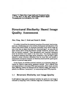
Fig. 1. Multi-scale structural similarity measurement system. L: low-pass filtering; 2 ↓: downsampling by 2. respectively. L is the dynamic range of the pixel values (L = 255 for 8 bits/pixel gray scale images), and K1 ¿ 1 and K2 ¿ 1 are two scalar constants. The general form of the Structural SIMilarity (SSIM) index between signal x and y is defined as: SSIM(x, y) = [l(x, y)]α · [c(x, y)]β · [s(x, y)]γ ,

(5)

where α, β and γ are parameters to define the relative importance of the three components. Specifically, we set α = β = γ = 1, and the resulting SSIM index is given by SSIM(x, y) =

(2 µx µy + C1 ) (2 σxy + C2 ) , (µ2x + µ2y + C1 ) (σx2 + σy2 + C2 )

(6)

which satisfies the following conditions:

Multi-scale method is a convenient way to incorporate image details at different resolutions. We propose a multi-scale SSIM method for image quality assessment whose system diagram is illustrated in Fig. 1. Taking the reference and distorted image signals as the input, the system iteratively applies a low-pass filter and downsamples the filtered image by a factor of 2. We index the original image as Scale 1, and the highest scale as Scale M , which is obtained after M − 1 iterations. At the j-th scale, the contrast comparison (2) and the structure comparison (3) are calculated and denoted as cj (x, y) and sj (x, y), respectively. The luminance comparison (1) is computed only at Scale M and is denoted as lM (x, y). The overall SSIM evaluation is obtained by combining the measurement at different scales using

1. symmetry: SSIM(x, y) = SSIM(y, x); 2. boundedness: SSIM(x, y) ≤ 1;

SSIM(x, y) = [lM (x, y)]αM ·

3. MULTI-SCALE STRUCTURAL SIMILARITY 3.1. Multi-scale SSIM index The perceivability of image details depends the sampling density of the image signal, the distance from the image plane to the observer, and the perceptual capability of the observer’s visual system. In practice, the subjective evaluation of a given image varies when these factors vary. A single-scale method as described in the previous section may be appropriate only for specific settings.

[cj (x, y)]βj [sj (x, y)]γj . (7)

j=1

3. unique maximum: SSIM(x, y) = 1 if and only if x = y. The universal image quality index proposed in [3] corresponds to the case of C1 = C2 = 0, therefore is a special case of (6). The drawback of such a parameter setting is that when the denominator of Eq. (6) is close to 0, the resulting measurement becomes unstable. This problem has been solved successfully in [5] by adding the two small constants C1 and C2 (calculated by setting K1 =0.01 and K2 =0.03, respectively, in Eq. (4)). We apply the SSIM indexing algorithm for image quality assessment using a sliding window approach. The window moves pixel-by-pixel across the whole image space. At each step, the SSIM index is calculated within the local window. If one of the image being compared is considered to have perfect quality, then the resulting SSIM index map can be viewed as the quality map of the other (distorted) image. Instead of using an 8 × 8 square window as in [3], a smooth windowing approach is used for local statistics to avoid “blocking artifacts” in the quality map [5]. Finally, a mean SSIM index of the quality map is used to evaluate the overall image quality.

M Y

Similar to (5), the exponents αM , βj and γj are used to adjust the relative importance of different components. This multiscale SSIM index definition satisfies the three conditions given in the last section. It also includes the single-scale method as a special case. In particular, a single-scale implementation for Scale M applies the iterative filtering and downsampling procedure up to Scale M and only the exponents αM , βM and γM are given nonzero values. To simplify parameter selection, we let αj =βj =γj for all j’s. In addition, we normalize the cross-scale settings such that PM γ =1. This makes different parameter settings (including j=1 j all single-scale and multi-scale settings) comparable. The remaining job is to determine the relative values across different scales. Conceptually, this should be related to the contrast sensitivity function (CSF) of the HVS [7], which states that the human visual sensitivity peaks at middle frequencies (around 4 cycles per degree of visual angle) and decreases along both high- and low-frequency directions. However, CSF cannot be directly used to derive the parameters in our system because it is typically measured at the visibility threshold level using simplified stimuli (sinusoids), but our purpose is to compare the quality of complex structured images at visible distortion levels. 3.2. Cross-scale calibration We use an image synthesis approach to calibrate the relative importance of different scales. In previous work, the idea of synthesizing images for subjective testing has been employed by the “synthesisby-analysis” methods of assessing statistical texture models, in

which the model is used to generate a texture with statistics matching an original texture, and a human subject then judges the similarity of the two textures [8]–[11]. A similar approach has also been qualitatively used in demonstrating quality metrics in [5], [12], though quantitative subjective tests were not conducted. These synthesis methods provide a powerful and efficient means of testing a model, and have the added benefit that the resulting images suggest improvements that might be made to the model [11]. 1

2

3

4

5

scale(M)

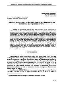
a specific distortion level (defined by MSE) and a specific scale. Each of the distorted image is created using an iterative procedure, where the initial image is generated by randomly adding white Gaussian noise to the original image and the iterative process employs a constrained gradient descent algorithm to search for the worst images in terms of SSIM measure while constraining MSE to be fixed and restricting the distortions to occur only in the specified scale. We use 5 scales and 12 distortion levels (range from 23 to 214 ) in our experiment, resulting in a total of 60 images, as demonstrated in Fig. 2. Although the images at each row has the same MSE with respect to the original image, their visual quality is significantly different. Thus the distortions at different scales are of very different importance in terms of perceived image quality. We employ 10 original 64×64 images with different types of content (human faces, natural scenes, plants, man-made objects, etc.) in our experiment to create 10 sets of distorted images (a total of 600 distorted images). We gathered data for 8 subjects, including one of the authors. The other subjects have general knowledge of human vision but did not know the detailed purpose of the study. Each subject was shown the 10 sets of test images, one set at a time. The viewing distance was fixed to 32 pixels per degree of visual angle. The subject was asked to compare the quality of the images across scales and detect one image from each of the five scales (shown as columns in Fig. 2) that the subject believes having the same quality. For example, one subject chose the images marked in Fig. 2 to have equal quality. The positions of the selected images in each scale were recorded and averaged over all test images and all subjects. In general, the subjects agreed with each other on each image more than they agreed with themselves across different images. These test results were normalized (sum to one) and used to calculate the exponents in Eq. (7). The resulting parameters we obtained are β1 = γ1 = 0.0448, β2 = γ2 = 0.2856, β3 = γ3 = 0.3001, β4 = γ4 = 0.2363, and α5 = β5 = γ5 = 0.1333, respectively. 4. TEST RESULTS

distortion level (MSE)

Fig. 2. Demonstration of image synthesis approach for cross-scale calibration. Images in the same row have the same MSE. Images in the same column have distortions only in one specific scale. Each subject was asked to select a set of images (one from each scale), having equal quality. As an example, one subject chose the marked images. For a given original 8bits/pixel gray scale test image, we synthesize a table of distorted images (as exemplified by Fig. 2), where each entry in the table is an image that is associated with

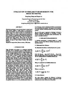
We test a number of image quality assessment algorithms using the LIVE database (available at [13]), which includes 344 JPEG and JPEG2000 compressed images (typically 768 × 512 or similar size). The bit rate ranges from 0.028 to 3.150 bits/pixel, which allows the test images to cover a wide quality range, from indistinguishable from the original image to highly distorted. The mean opinion score (MOS) of each image is obtained by averaging 13∼25 subjective scores given by a group of human observers. Eight image quality assessment models are being compared, including PSNR, the Sarnoff model (JNDmetrix 8.0 [14]), singlescale SSIM index with M equals 1 to 5, and the proposed multiscale SSIM index approach. The scatter plots of MOS versus model predictions are shown in Fig. 3, where each point represents one test image, with its vertical and horizontal axes representing its MOS and the given objective quality score, respectively. To provide quantitative performance evaluation, we use the logistic function adopted in the video quality experts group (VQEG) Phase I FR-TV test [15] to provide a non-linear mapping between the objective and subjective scores. After the non-linear mapping, the linear correlation coefficient (CC), the mean absolute error (MAE), and the root mean squared error (RMS) between the subjective and objective scores are calculated as measures of prediction accuracy. The prediction consistency is quantified using the outlier ratio (OR), which is de-

Table 1. Performance comparison of image quality assessment models on LIVE JPEG/JPEG2000 database [13]. SS-SSIM: single-scale SSIM; MS-SSIM: multi-scale SSIM; CC: non-linear regression correlation coefficient; ROCC: Spearman rank-order correlation coefficient; MAE: mean absolute error; RMS: root mean squared error; OR: outlier ratio. Model PSNR Sarnoff SS-SSIM (M=1) SS-SSIM (M=2) SS-SSIM (M=3) SS-SSIM (M=4) SS-SSIM (M=5) MS-SSIM

CC 0.905 0.956 0.949 0.963 0.958 0.948 0.938 0.969

ROCC 0.901 0.947 0.945 0.959 0.956 0.946 0.936 0.966

MAE 6.53 4.66 4.96 4.21 4.53 4.99 5.55 3.86

RMS 8.45 5.81 6.25 5.38 5.67 6.31 6.88 4.91

OR(%) 15.7 3.20 6.98 2.62 2.91 5.81 7.85 1.16

fined as the percentage of the number of predictions outside the range of ±2 times of the standard deviations. Finally, the prediction monotonicity is measured using the Spearman rank-order correlation coefficient (ROCC). Readers can refer to [15] for a more detailed descriptions of these measures. The evaluation results for all the models being compared are given in Table 1. From both the scatter plots and the quantitative evaluation results, we see that the performance of single-scale SSIM model varies with scales and the best performance is given by the case of M=2. It can also be observed that the single-scale model tends to supply higher scores with the increase of scales. This is not surprising because image coding techniques such as JPEG and JPEG2000 usually compress fine-scale details to a much higher degree than coarse-scale structures, and thus the distorted image “looks” more similar to the original image if evaluated at larger scales. Finally, for every one of the objective evaluation criteria, multi-scale SSIM model outperforms all the other models, including the best single-scale SSIM model, suggesting a meaningful balance between scales. 5. DISCUSSIONS We propose a multi-scale structural similarity approach for image quality assessment, which provides more flexibility than singlescale approach in incorporating the variations of image resolution and viewing conditions. Experiments show that with an appropriate parameter settings, the multi-scale method outperforms the best single-scale SSIM model as well as state-of-the-art image quality metrics. In the development of top-down image quality models (such as structural similarity based algorithms), one of the most challenging problems is to calibrate the model parameters, which are rather “abstract” and cannot be directly derived from simple-stimulus subjective experiments as in the bottom-up models. In this paper, we used an image synthesis approach to calibrate the parameters that define the relative importance between scales. The improvement from single-scale to multi-scale methods observed in our tests suggests the usefulness of this novel approach. However, this approach is still rather crude. We are working on developing it into a more systematic approach that can potentially be employed

in a much broader range of applications. 6. REFERENCES [1] A. M. Eskicioglu and P. S. Fisher, “Image quality measures and their performance,” IEEE Trans. Communications, vol. 43, pp. 2959–2965, Dec. 1995. [2] T. N. Pappas and R. J. Safranek, “Perceptual criteria for image quality evaluation,” in Handbook of Image and Video Proc. (A. Bovik, ed.), Academic Press, 2000. [3] Z. Wang and A. C. Bovik, “A universal image quality index,” IEEE Signal Processing Letters, vol. 9, pp. 81–84, Mar. 2002. [4] Z. Wang, H. R. Sheikh, and A. C. Bovik, “Objective video quality assessment,” in The Handbook of Video Databases: Design and Applications (B. Furht and O. Marques, eds.), pp. 1041–1078, CRC Press, Sept. 2003. [5] Z. Wang, A. C. Bovik, H. R. Sheikh, and E. P. Simoncelli, “Image quality assessment: From error measurement to structural similarity,” IEEE Trans. Image Processing, vol. 13, Jan. 2004. [6] Z. Wang, L. Lu, and A. C. Bovik, “Video quality assessment based on structural distortion measurement,” Signal Processing: Image Communication, special issue on objective video quality metrics, vol. 19, Jan. 2004. [7] B. A. Wandell, Foundations of Vision. Sinauer Associates, Inc., 1995. [8] O. D. Faugeras and W. K. Pratt, “Decorrelation methods of texture feature extraction,” IEEE Pat. Anal. Mach. Intell., vol. 2, no. 4, pp. 323–332, 1980. [9] A. Gagalowicz, “A new method for texture fields synthesis: Some applications to the study of human vision,” IEEE Pat. Anal. Mach. Intell., vol. 3, no. 5, pp. 520–533, 1981. [10] D. Heeger and J. Bergen, “Pyramid-based texture analysis/synthesis,” in Proc. ACM SIGGRAPH, pp. 229–238, Association for Computing Machinery, August 1995. [11] J. Portilla and E. P. Simoncelli, “A parametric texture model based on joint statistics of complex wavelet coefficients,” Int’l J Computer Vision, vol. 40, pp. 49–71, Dec 2000. [12] P. C. Teo and D. J. Heeger, “Perceptual image distortion,” in Proc. SPIE, vol. 2179, pp. 127–141, 1994. [13] H. R. Sheikh, Z. Wang, A. C. Bovik, and L. K. Cormack, “Image and video quality assessment research at LIVE,” http://live.ece.utexas.edu/ research/quality/. [14] Sarnoff Corporation, “JNDmetrix Technology,” http: //www.sarnoff.com/products_services/ video_vision/jndmetrix/. [15] VQEG, “Final report from the video quality experts group on the validation of objective models of video quality assessment,” Mar. 2000. http://www.vqeg.org/.

100

100 JPEG images JPEG2000 images Fitting with Logistic Function

80

80

70

70

60

60

50

50

40

40

30

30

20

20

10 0 15

JPEG images JPEG2000 images Fitting with Logistic Function

90

MOS

MOS

90

10 20

25

30

35

40

45

0 0

50

2

4

PSNR

(a)

80 70

60

60 MOS

MOS

90

70

50

40

30

30

20

20

10

10

0.4

0.5 0.6 0.7 0.8 Single−scale SSIM (M=1)

0.9

0 0.5

1

JPEG images JPEG2000 images Fitting with Logistic Function

0.6

0.7 0.8 Single−scale SSIM (M=2)

(c)

80 70

60

60 MOS

MOS

90

70

50

40

30

30

20

20

10

10 0.75

0.8 0.85 0.9 Single−scale SSIM (M=3)

0.95

JPEG images JPEG2000 images Fitting with Logistic Function

50

40

0 0.85

1

0.9 0.95 Single−scale SSIM (M=4)

(e) 100 JPEG images JPEG2000 images Fitting with Logistic Function

90

80

80

70

70

60

60 MOS

MOS

1

(f)

100

50

40

30

30

20

20

10

10 0.93

0.94

0.95 0.96 0.97 0.98 Single−scale SSIM (M=5)

(g)

0.99

1

JPEG images JPEG2000 images Fitting with Logistic Function

50

40

0 0.92

1

100 JPEG images JPEG2000 images Fitting with Logistic Function

80

90

0.9

(d)

100

0 0.7

12

50

40

90

10

100

JPEG images JPEG2000 images Fitting with Logistic Function

80

0 0.3

8

(b)

100 90

6 Sarnoff

0 0.7

0.75

0.8

0.85 0.9 Multi−scale SSIM

0.95

1

(h)

Fig. 3. Scatter plots of MOS versus model predictions. Each sample point represents one test image in the LIVE JPEG/JPEG2000 image database [13]. (a) PSNR; (b) Sarnoff model; (c)-(g) single-scale SSIM method for M = 1, 2, 3, 4 and 5, respectively; (h) multi-scale SSIM method.