Multiagent Learning for Open Systems: A Study in

Multiagent Learning for Open Systems: A Study in Opponent Classification Michael Rovatsos, Gerhard Weiß, and Marco Wolf {rovatsos,weissg,wolf}@in.tum.de Department of Informatics Technical University of Munich 85748 Garching bei München Germany

Abstract. Open systems are becoming increasingly important in a variety of distributed, networked computer applications. Their characteristics, such as agent diversity, heterogeneity and fluctuation, confront multiagent learning with new challenges. This paper presents the interaction learning meta-architecture InFFrA as one possible answer to these challenges, and introduces the opponent classification heuristic A D H OC as a concrete multiagent learning method that has been designed on the basis of InFFrA. Extensive experimental validation proves the adequacy of A D H OC in a scenario of iterated multiagent games and underlines the usefulness of schemas such as InFFrA specifically tailored for open multiagent learning environments. At the same time, limitations in the performance of A D H OC suggest further improvements to the methods used here. Also, the results obtained from this study allow more general conclusions regarding the problems of learning in open systems to be drawn.

1 Introduction The advent of the Internet brought with it an increasing interest in open systems [8, 10]. Real-world applications such as Web Services, ubiquitous computing, web-based supply chain management, peer-to-peer systems, ad hoc networks for mobile computing etc. involve interaction between users (humans, mobile devices, companies) with different goals whose internal structure is intransparent for others. Agent populations change dynamically over time. Drop-outs, malicious agents and agents who fail to complete tasks assigned to them may jeopardise the robustness of the overall system. Centralised authorities and “trusted third parties” are (if they exist at all) not always trustworthy themselves, since ultimately they are also serving someone’s self-interest. Obviously, these phenomena confront multiagent systems (MAS) [19] research with new challenges, because many assumptions regarding the knowledge of agents about each other are no more realistic. While the MAS community as a whole has been concentrating on relatively closed systems for a long time, multiagent learning researchers have long dealt with the problems of openness. This is because of the characteristic of machine learning [12] approaches in general to look at problems of acquiring useful knowledge from observation in complex domains in which this knowledge is not readily available. Thus, it is only natural to take a learning approach to build intelligent, flexible

and adaptive agents that can operate in open systems – in fact, the amount of potentially “missing” knowledge offers a seemingly endless source of new learning problems that need to be tackled. Mostly, the purpose of applying learning techniques in the construction of adaptive agents is to learn how to predict the behaviour of the system one way or the other. As far as multiagent learning is concerned, this means learning how to predict the behaviour of other agents, e.g. by learning their preferences [2], their strategies [3, 6, 17], the outcomes of joint actions or all of these [15], i.e. in some way to acquire a model of the opponent1. Most of the time, these models are also used to derive an optimal strategy towards this opponent at the same time, such as in [5, 3, 6, 15]. The majority of these multiagent learning approaches adopt a heavily cognitionbiased view of learning, which aims at extracting as much information from observation as possible about an individual. However, in large-scale, open MAS, in which agents have only occasional encounters with peers they are acquainted with, learning models of individual peer agents may not be feasible. This is because the cost of acquiring and maintaining an adequate model of the other normally outweighs its potential benefits if the probability of interacting with that same agent in the future is not very high. This problem has lead us to investigate a more social view of multiagent learning that is more adequate for open systems, which, at its core, focuses around the idea of learning the behaviour of agents in certain classes of interactions rather than the specific properties of particular agents. At the level of architectures for social learning of this kind, we have developed InFFrA [14] which provides a meta-model for developing appropriate learning algorithms. In this paper, we present a concrete implementation of this model for the problem of learning in multi-agent games called A D H OC (Adaptive Heuristic for Opponent Classification) and illustrate its usefulness by providing extensive experimental results. These confirm our initial intuition that the road to the development of new multiagent learning methods for open systems is long, but that our methodology is a first step in the right direction. The remainder of this paper is structured as follows: we first introduce our general intuitions about learning in open systems (section 1). Subsequently, section 2 presents an abridged introduction to the InFFrA social learning architecture. Section 3 then introduces A D H OC, an application of InFFrA to learning in multi-player games and section 4 presents extensive experimental results obtained from A D H OC simulations. In section 5, we discuss these results and make suggestions for further improvements, and section 6 concludes.

2 Open Systems: A New Challenge for Multiagent Learning One of the most prominent problems multiagent learning (MAL) research deals with is how to build an agent who can learn to perform optimally in a given environment. We will restrict the scope of our analysis to a sub-class of this problem, in which we are more specifically concerned with building an optimal “goal-rational agent” by assuming 1

We will make frequent use of the terms opponent, adversary, peer, partner etc. They are all intended to mean “other agent” without any implications regarding the competitive or cooperative nature of the interactions.

that an agent has preferences regarding different states of affairs and that she deliberates in order to reach those states of the world that seem most desirable to her (usually, these preferences are expressed by a utility function or an explicit set of goals/tasks). The environment such an agent is situated in is assumed to be co-inhabited by other agents that the agent interacts with. We assume that, in general, agents’ actions have effects on each other’s goal attainment so that agents have to coordinate their actions with each other to perform well. In the absence of omnipotence, it is useful and often necessary for agents to organise their experience in a cause-and-effect model of some sort in order to be able to adapt to the environment and to take rational action; only if the rules that govern the world are discovered can an agent actively pursue its goals through means-ends-reasoning, because such means-ends-reasoning requires making predictions about the effects of one’s own actions. Such a model of the world should not only capture the properties of the physical environment, but also describe (and predict) the behaviour of other agents, as they also influence the outcome of certain activities. In our analysis, we concentrate on the latter problem and neglect all problems associated with learning to behave optimally in a (passive) environment. This is to say that our focus is on agents that model other agents in order to predict the future behaviour of those agents. While the activity of modelling other agents forms part of virtually any “socially adaptive” agent design, open MAS have some special characteristics that add to the complexity of this modelling activity: 1. Behavioural diversity: In open systems, agents are usually granted (deliberately or inevitably) more degrees of freedom in their behaviour. For example, they might be untruthful, malicious or not behaving rationally from the modelling agent’s perspective. Generally speaking, an agent that is trying to model other agents can make less a priori assumptions about the internals or the behaviour of other agents (such as the benevolence and rationality assumptions in the above examples). In machine learning terms, this means that the hypothesis space [12] used when learning about others will be larger than it is in closed systems. 2. Agent heterogeneity: Open systems allow for a larger variety of possible agent designs than closed systems do. One problem this leads to is that an agent who is building models of other agents will need to maintain many different models. Worse still, it might be the case that the modelling agent has to apply different learning methods for different peers (for example, a logic-based adversary might be better modelled using inductive logic programming while decision tree learning might be better when modelling a reactive opponent). 3. Agent fluctuation: If agents may freely enter and leave the system, it is not clear how the agent should assess the value of learning a model of them. This makes it very hard to estimate how much effort should be spent on learning models of particular agents (given that the agent has only limited resources some of which it also needs for perception, planning and execution), considering that information about certain agents might become useless anytime. A side-effect of this is also that it becomes much harder to develop a reasonable “exploration vs. exploitation” strategy, not knowing which partners deserve being “explored”.

Taken together, these phenomena might be seen as different aspects of what can be called the contingent acquaintances problem (CAP) of modelling other agents: the problem that the behaviours of known peers are unrestricted, that there are many different agents the modelling agent is acquainted with, and that there is uncertainty about the value of information obtained from learning more about these acquaintances. Although opponent modelling (OM) has received considerable attention from the multiagent learning community in recent years, we feel that this problem has been largely ignored. Our own research has been focusing on a specific approach that addresses the CAP by different means called interaction frame learning. Essentially, it is based on the idea of learning different categories of interactions instead of particular models of individual adversaries, while combining learned patterns of behaviour appropriately with information about some specific individual agent whenever such information is available.

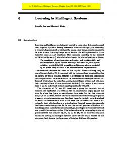
3 InFFrA: A Meta-Architecture for Social Learning InFFrA (the Interaction Frames and Framing Architecture) is a sociologically informed framework for building social learning and reasoning architectures. It is based on the concepts of “interaction frames” and “framing” which originate in the work of Erving Goffman [9]. Essentially, interaction frames describe classes of interaction situations and provide guidance to the agent about how to behave in a particular social context. Framing, on the other hand, signifies the process of applying frames in interaction situations appropriately. As Goffman puts it, framing is the process of answering the question “what is going on here?” in a given interaction situation – it enables the agent to act in a competent, routine fashion. In a MAL context, interaction frames can be seen as learning hypotheses that contain information about interaction situations. This information should suffice to structure interaction for the individual that employs the frames. Also, frames describe recurring categories of interaction rather than the special properties of individual agents, as most models learned by OM techniques.Thus, learning interaction frames is suitable to cope with the class of learning problems described in the previous section. A brief overview of InFFrA will suffice for the purposes of this paper and hence we will not go into its details here. More complete accounts can be found in [14] and [16]. In their computationally operationalised version, frames are data structures which contain information about – the possible interaction trajectories (i.e. the courses the interaction may take in terms of sequences of actions/messages), – roles and relationships between the parties involved in an interaction of this type, – contexts within which the interaction may take place (states of affairs before, during, and after an interaction is carried out) and – beliefs, i.e. epistemic states of the interacting parties. Figure 1 shows a graphical representation for the interaction frame (henceforth “frame”) data structure. As examples for how the four “slots” of information it provides might be realised, it contains graphical representations of groups (boxes) and relationships

Frame trajectories

roles & relationships R1

R2

R3

G2 A1

R2

A7

status

R3

A7

A2 A6

A9

A4

G1

context preconditions

trajectory model

beliefs postconditions

conceptual beliefs

A R2

time

C9

E

C

C4 R2

C8

C5

G

F R1

C3

D

B

R3

C1

C2

A8

A3

R5

R4

time

A5

R1

C10

activation conditions

deactivation conditions

A

R3 B

G

D

C C6

R1

C7

sustainment conditions

causal beliefs

F E

H

Fig. 1. Interaction frame data structure.

(arrows) in the “roles and relationships” slot and a protocol-like model of concurrent agent actions in the “trajectories” slot. The “contexts” slot embeds the trajectory model in boxes that contain preconditions, postconditions and conditions that have to hold during execution of the frames. The “beliefs” slot contains a semantic network and a belief network as two possible representations of ontological and causal knowledge, where shaded boxes define which parts of the networks are known to which participant of the frame. A final important characteristic of frames is that certain attributes of the above must be assumed to be shared knowledge among interactants (so-called common attributes) for the frame to be carried out properly while others may be private knowledge of the agent who “owns” the frame (private attributes). Private attributes are mainly used by agents to store their personal experience with a frame, e.g. utilities associated with previous frame enactments and instance values for the variables used in generic representations that describe past enactments (“histories”), inter-frame relationships (“links”) etc. Apart from the interaction frame abstraction, InFFrA also offers a control flow model for social reasoning and social adaptation based on interaction frames, through which an InFFrA agent performs its framing. Before describing the steps that are performed in this reasoning cycle, we need to introduce the data structures on which they operate. They are - the active frame (the unique frame currently activated),

InFFrA Framing Architecture

frame repository

F2

F1

action

behaviour generation module

perceived frame

frame enactment module

activated frame

F

trajec− tory

situation interpretation module

Fn F

F

frame adjustment module

retain

adapt

contexts beliefs compliance

perception

F

difference model roles

F

F3 .....

F

deviance

frame matching module

framing assessment module

sub−social level private goals/values

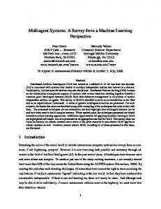
Fig. 2. Detailed view of the framing-based agent architecture. The main line of reasoning between perception and action (shown as a shaded arrow) captures both the sub-processes involved and the temporal order in which they occur.

- the perceived frame (a frame-wise interpretation of the currently observed state of affairs), - the difference model (containing the differences between perceived frame and active frame), - the trial frame (the current hypothesis when alternatives to the current frame are sought for), - and the frame repository, a (suitably organised) frame database used as a hypothesis space. The control flow model consists of the following steps: 1. Matching: Compare the current interaction situation (the perceived frame) with the frame that is currently being used (the active frame). 2. Assessment: Assess the usability of the current active frame. 3. Framing decision: If the current frame seems appropriate, retain the active frame and continue with 6. Else, proceed with 4. to find a more suitable frame. 4. Re-framing: Search the frame repository for more suitable frames. If candidates are found, “mock-activate” one of them as a trial frame and go back to 1; else, proceed with 5. 5. Adaptation: Iteratively modify frames in the frame repository and continue with 4. If no candidates for modification can be found, create a new frame on the grounds of the perceived frame.

6. Enactment: Influence action decisions by applying the active frame. Return to 1. Figure 2 visualises the steps performed in this reasoning cycle. It introduces a functional module for each of the above steps and shows how these modules operate on the active/perceived/trial frame, difference model and frame repository data structures. Also, it links the sub-social reasoning (e.g. BDI [13]) level to the InFFrA layer by suggesting that the agent’s goals and preferences are taken into account in the frame assessment phase. InFFrA offers a number of advantages regarding the design of social learning techniques for open learning environments: 1. The frame abstraction combines information about all the relevant aspects of a certain class of interaction. It contains information about who is interacting, what they are expected (not) to do when they interact, when they will apply this frame and what they need to know to carry out the frame appropriately. At the same time, it is left to the particular algorithm designed with InFFrA to specify which of these aspects it will focus on and how they will be modelled. For example, beliefs can be completely disregarded in scenarios in which behavioural descriptions are considered sufficient. 2. The framing procedure addresses all issues relevant to the design of interaction learning algorithms. It assists the designer in the analysis of – what knowledge should be captured by the frames and which level of abstraction should be chosen for them, – how perception is to be interpreted and matched against existing conceptions of frames, – how to define an implementable criterion for retaining or rejecting a frame, – which operators will be used for retrieving, updating, generating and modifying frames in the repository, – how the concrete behaviour of the agent should be influenced by frame activation (in particular, how local goal-oriented decision-making should be combined with social considerations). 3. It provides a unifying view for various perspectives on social learning at the interaction level. By touching upon classical machine learning issues such as classification, active learning, exploration vs. exploration, case-based methods, reinforcement and the use of prior knowledge, InFFrA provides a complete learning view of interaction. This enables us to make the relationship of specific algorithms to these issues explicit, if the algorithms have been developed (or analysed) with InFFrA. In the following section, we will lay out the process of applying the InFFrA framework in the design of a MAL system for opponent classification.

4

A D H OC

InFFrA has been successfully used to develop the A Daptive Heuristic for Opponent Classification A D H OC which addresses the problem of learning opponent models in

the presence of large numbers of opponents. This is a highly relevant problem in open systems, because encounters with particular adversaries are only occasional, so that the an agent will usually encounter peers it knows nothing of. Therefore, hoping that opponents will only use a limited set of strategies is the only possibility of learning anything useful at all, and hence it is only natural to model classes of opponents instead of individuals. Remarkably, this issue has been largely overlooked by research on opponent modelling. Yet, this area abounds in methods for learning models of particular individuals’ strategies (cf. [2, 5, 3, 6, 15]). Therefore, proposing new OM methods was not an issue by itself in the development of A D H OC. Instead, the classification method was thought to be parametrised with some OM method in concrete implementations. In fact, A D H OC does not depend on any particular choice of OM method, as long as the opponent models fulfil certain criteria. For our experimental evaluation in an iterated multiagent game-playing scenario, we combined A D H OC with the well-known US-L* algorithm proposed by Carmel and Markovitch [4, 3]. This algorithm is based on modelling opponent strategies in terms of deterministic finite automata (DFA) which can then be used to learn an optimal counterstrategy, e.g. by using standard Q-learning [18]. In explaining the system, we will first give an overview of A D H OC, then explain the underlying models and algorithms, and finally describe how it can be combined with the US-L* algorithm. 4.1 Overview A D H OC creates and maintains a bounded, dynamically adapted number of opponent classes C = {c1 , . . . ck } in a society of agents A = {a1 , . . . an } together with a (crisp) agent-class membership function m : A → C that denotes which class any known agent aj pertains to from the perspective of a modelling agent ai . In our application of A D H OC to multiagent iterated games, each of this classes will consist of (i) a DFA that represents the strategy of opponents assigned to it (this DFA is learned using the USL* algorithm), (ii) a Q-value table that is used for evolving an optimal counter-strategy against this behaviour and (iii) a set of most recent interactions with this class. This instance of A D H OC complies with the more general assumptions that have to be made regarding any OM method that is used – it allows for the derivation of an opponent model and it makes the use of this model possible in order to achieve optimal behaviour towards this kind of opponent. A D H OC assumes that interaction takes place between only two agents at a time in discrete encounters e = h(s0 , t0 ), . . . (sl , tl )i of length l where sk and tk are the actions of ai and aj in each round, respectively. Each pair (sk , tk ) is associated with a real-valued utility ui for agent ai 2 . The top-level A D H OC algorithm operates on the following inputs: - an opponent aj that ai is currently interacting with, 2

Any encounter can be interpreted as a fixed length iterated two-player normal-form game [7]; however, the OM method we use in our implementation does not require that ui be a fixed function that returns the same payoff for every enactment of a joint action (sk , tk ) (in contrast to classical game-theoretic models of iterated games).

- the behaviour of both agents in the current encounter e (we assume that A D H OC is called after the encounter is over) and - an upper bound k on the maximal size of C. It maintains and modifies the values of - the current set of opponent classes C = {c1 , . . . ck } (initially C = ∅) and - the current membership function m : A → C ∪ {⊥} (initially undefined (⊥) for all agents). Thus, assuming that an OM method is available for any c = m(aj ) (obtained via the function OM (c)) which provides aj with methods for optimal action determination, the agent can use that model to plan its next steps. In InFFrA terms, each A D H OC class is an interaction frame. In a given encounter, the modelling agent matches the current sequence of opponent moves with the behavioural models of the classes in C (situation interpretation and matching). It then determines the most appropriate class for the adversary (assessment). In A D H OC, this is done using a similarity measure S between adversaries and classes. After an encounter, the agent may have to revise its framing decision: If the current class does not cater for the current encounter, the class has to be modified (frame adaptation), or a better class has to be retrieved from C (re-framing). If no adequate alternative is found or frame adaptation seems inappropriate, a new class has to be generated that matches the current encounter. In order to determine its own next action, the agent applies the counterstrategy learned for this particular opponent model (behaviour generation). Feedback obtained from the encounter is used to update the hypothesis about the agent’s optimal strategy towards the current opponent class. A special property of A D H OC is that is combines the two types of opponent modelling previously discussed, i.e. the method of learning something about particular opponents versus the method of learning types of behaviours or strategies that are relevant for more than one adversary. It does so by distinguishing between opponents the agent is acquainted with and those it encounters for the first time. If an unknown peer is encountered, that agent determines the optimal class to be chosen after each move in the iterated game, possibly revising its choice over and over again. Else, the agent uses its experience with the peer by simply applying the counter-strategy suggested by the class that this peer had previously been assigned to. Next, we will describe how all this is realised in A D H OC in more detail. 4.2 The Heuristic in Detail Before presenting the top-level heuristic itself, we first have to introduce O PTA LTC LASS, a function for determining the most suitable class for an opponent after a new encounter which is employed in several situations in the top-level A D H OC algorithm. A pseudo-code description of this function is given in algorithm 1. The O PTA LT C LASS procedure proceeds as follows: if C is empty, a new class is created whose opponent model is consistent with e (function N EW C LASS). Else, a set of maximally similar classes Cmax is computed, the similarity of which with the behaviour

Algorithm 1 procedure O PTA LT C LASS inputs: Agent aj , Encounter e, Set C, Int k, Int b outputs: Class c begin if C 6= ∅ then {Compute the set of classes that are most similar to aj , at least with similarity b } Cmax = {c|S(aj , c) = maxc0 ∈C S(aj , c0 ) ∧ S(aj , c) ≥ b} if Cmax 6= ∅ then {Return the “best” of the most similar classes} return arg maxc∈Cmax Q UALITY(c) else {Create a new class, if |C| permits; else, the “high similarity” condition is dropped} if |C| < k then return N EW C LASS(e) else return O PTA LT C LASS(C, k, −∞) end if end if else return N EW C LASS(e) end if end

of aj must be at least b (we explain below how this threshold is used in the top-level heuristic). The algorithm strongly relies on the definition a similarity measure S(aj , c) that reflects how accurate the predictions of c regarding the past behaviour of a j are. In our prototype implementation, the value of S is computed as the ratio between the number of encounters with aj correctly predicted by the class and the number of total encounters with aj (where only entirely correctly predicted action sequences count as “correct” predictions, i.e. a single mis-predicted move suffices to reject the prediction of a particular class). As we well see below in the description of the top-level algorithm, this definition of S does not require entire encounters with aj to be stored (which would contradict our intuition that less attention should be paid to learning data associated with individual peers). Instead, the modelling agent can simply keep track of the ratio of successful predictions by incrementing counters. If Cmax is empty, a new class has to be generated for aj . However, this is only possible if the size of C does not exceed k, because, as mentioned before, we require the set of opponent classes to be bounded in size. If C has already reached its maximal size, O PTA LT C LASS is called with b = −∞, so that the side-condition of S(a j , c) ≥ b can be dropped if necessary. If Cmax is not empty, i.e. there exist several classes with identical (maximal) similarity, we pick the best class according to the heuristic function Q UALITY, which may use any additional information regarding the reliability or computational cost of classes.

In our implementation, this function is defined as follows: Q UALITY(c) = α · +γ·

#CORRECT(c) + #ALL(c) #agents(c) #known_agents

β·

#corr(c) #all(c)

1 + (1 − α − β − γ) · C OST (C)

where - #ALL(c) is the total number of all predictions of class c in all past games, - #CORRECT(c) is the total number of correct predictions of class c in all past games, - #all(c) is the total number of all predictions of class c in the current encounter, - #correct(c) is the total number of correct predictions of class c in the current encounter, - #agents(c) = |{a ∈ A|m(a) = c}|, - #known_agents be the number of known agents, - C OST ( C ) is a measure for the size of the model OM (c) and - α + β + γ ≤ 1. Thus, we consider those classes to be most reliable and efficient that are 1. accurate in past and current predictions (usually, α < β); 2. that account for a great number of agents (i.e. that have a large “support”); 3. that are small in size, and hence computationally cheap. It should be noted that the definition of a Q UALITY function is not a critical choice in our implementation of A D H OC, since it is only used to obtain a deterministic method of optimal class selection in case several classes have exactly the same similarity value for the opponent in question (a rather unlikely situation). If the similarity measure is less fine-grained, though, such a “quality” heuristic might significantly influence the optimal class choice. Given the O PTA LT C LASS function that provides a mechanism to re-classify agents, we can now present the top-level A D H OC heuristic. Apart from the inputs and outputs already described in the previous paragraphs, it depends on a number of additional internal parameters: - an encounter comprehension flag ecf(c) that is true, whenever the opponent model of some class c “understands” (i.e. would have correctly predicted) the current encounter; - an “unchanged” counter u(c) that counts the number of past encounters (across opponents) for which the model for c has remained stable; - a model stability threshold τ that is used to determine very stable classes; - similarity thresholds δ, ρ1 and ρ2 that similarities S(a, c) are compared against to determine when an agent needs to be re-classified and which classes it might be assigned to.

Algorithm 2 A D H OC top-level heuristic inputs: Agent aj , Encounter e, Integer k outputs: Set C, Membership function m begin c ← m(aj ) {The similarity values of all classes are updated depending on their prediction accuracy regarding e} for all c ∈ C do correct(aj ,c) S(aj , c) ← all(aj ) end for if c = ⊥ then {Unknown aj is put into the best sufficiently similar class that understands at least e, if any; else, a new class is created, if k permits} m(aj ) ← O PTA LT C LASS(C, k, aj , 1) if m(aj ) 6∈ C then C ← C ∪ {m(aj )} end if else {c is incorrect wrt aj or very stable} if S(aj , c) ≤ δ ∨ u(c) ≥ τ then {Re-Classify aj to a highly similar c, if any; else create a new class if k permits} m(aj ) ← O PTA LT C LASS(C, k, aj , ρ1 ) if m(aj ) 6∈ C then C ← C ∪ {m(aj )} end if else {The agent is re-classified to the maximally similar (if also very stable) class} c0 ← O PTA LT C LASS(C, k, aj , ρ2 ) if c0 ∈ C ∧ u(c0 ) > τ then m(aj ) ← c0 end if end if O M -L EARN(m(aj ), e) {Model of m(aj ) was modified because of e} if ecf(m(aj )) = false then {Reset similarities for all non-members of c} for all a0 ∈ A do if m(a0 ) 6= c then S(a0 , c) ← 0 end if end for end if C ← C − {c0 |∀a.m(a) 6= c0 } end if

After completing an encounter with opponent aj , the heuristic proceeds as presented in the pseudo-code description of algorithm 2. At the beginning, we set the current class c to the value of the membership function for opponent aj . So in case of encountering a known agent, the modelling agent makes use of her prior knowledge about aj . Then, we update all classes’ current similarity values with respect to aj as described above, i.e. by dividing the number of past encounters with aj that would have been correctly predicted by class c (correct(a j , c)) by the total number of past encounters with aj (all(aj )). In InFFrA terms, the similarity function represents the difference model, and thus, A D H OC keeps track of the difference between all opponents’ behaviours and all frames simultaneously. Therefore, the assessment phase in the framing procedure simply consists of consulting the similarity values previously computed. In other words, the complexity of assessing the usability of a particular frame in an interaction situation is shifted to the situation interpretation and matching phase. If aj has just been encountered for the first time, the value of m(aj ) is undefined (this is indicated by the condition c = ⊥). Quite naturally, aj is put into the best class that correctly predicts the data in the current encounter e, since the present encounter is the only available source of information about the behaviour of a j . Since only one sample e is available for the new agent, setting b = 1 in O PTA LT C LASS amounts to requiring that candidate classes correctly predict e. Note, however, that this condition will be dropped inside O PTA LT C LASS, if necessary (i.e. if no class correctly predicts the encounter). In that case, that class will be chosen for which Q UALITY (c) is maximal. Again, taking an InFFrA perspective, this means that a (reasonably general and cheap) frame that is consistent with current experience is activated. If no such frame is available, the current encounter data is used to form a new category unless no more “agent types” can be stored. It should be noted that this step requires the OM method to be capable of producing a model that is consistent at least with a single observed encounter. Next, consider the case in which m(aj ) 6= ⊥, i.e. the case in which the agent has been classified before. In this case, we have to enter the re-classification routine to improve the classification of aj , if this is possible. To this end, we choose to assign a new class to aj , if the similarity between agent aj and its current class c falls below some threshold δ or if the model c has remained stable for a long time (u(c) ≥ τ ) (which implies that it is valuable with respect to predictions about other agents). Also, we require that candidate classes for this re-classification be highly similar to aj (b = ρ1 ). As before, if no such classes exist, O PTA LT C LASS will generate a new class for a j , and if this is not possible, the “high similarity” condition is dropped – we simply have to classify aj one way or the other. In the counter-case (high similarity and unstable model), we still attempt to pick a new category for aj . This time, though, we only consider classes that are very stable, very similar to aj (ρ2 > ρ1 ), and we ignore classes output by O PTA LT C LASS that are new (by checking “if c0 ∈ C . . .”). The intuition behind this is to merge similar classes in the long run so as to obtain a minimal C. After re-classification, we update the class m(aj ) by calling its learning algorithm O M -L EARN and using the current encounter e as a sample. The “problem case” occurs

if e has caused changes to model c because of errors in the predicted behaviour of a j (ecf(m(aj )) = false), because in this case, the similarity values of m(aj ) to all agents are no more valid. Therefore, we choose to set the similarities of all non-members of c with that class to 0, following the intuition that since c has been modified, we cannot make any accurate statement about the similarity of other agents with it (remember that we do not store past encounters for each known agent and are hence unable to re-assess the values of S). Finally, we erase all empty classes from C. To sum up, the heuristic proceeds as follows: it creates new classes for unknown agents or assigns them to “best matches” classes if creating new ones is not admissible. After every encounter, the best candidate classes for the currently encountered agent are those that are able to best predict past encounters with it. At the same time, good candidates have to be models that have been reliable in the past and low in computational cost. Also, classes are merged in the long run if they are very similar and very stable. With respect to InFFrA, assigning agents to classes and creating new classes defines the re-framing and frame adaptation details. Merging classes and deleting empty classes, on the other hand, implements a strategy of long-term frame repository management. As far as action selection is concerned, a twofold strategy is followed: in the case of known agents, agent ai simply uses OM (m(aj )) when interacting with agent aj , and the classification procedure is only called after an encounter e has been completed. If an unknown agent is encountered, however, the most suitable class is chosen for action selection in each turn using O PTA LT C LASS. This reflects the intuition that the agent puts much more effort into classification in case it interacts with a new adversary, because it knows very little about that adversary. In the following section we introduce the scenario we have chosen for an empirical validation of the heuristic. This section will also present the details of combining A D H OC with a concrete OM method for a given application domain.

5 Application to Iterated Multiagent Games To evaluate A D H OC, we choose the long-studied domain of iterated multiagent games that captures a number of interesting interaction issues. More specifically, we implemented a simulation system in which agents move on a toroidal grid and play a fixed number of Iterated Prisoner’s Dilemma [7, 11] games whenever they happen to be in the same caret with some other agent. The matrix for the single-shot Prisoner’s Dilemma game in normal form is given in Table 1. If more than two agents meet, every player plays against every other player where couplings are drawn in random order. As stated before, we extend the model-based learning method US-L* proposed by Carmel and Markovitch [4, 3] that is based on learning opponent behaviour in terms of a DFA by classification capabilities. To this end, we model the opponent classes used in A D H OC as follows: let C = {ci = hAi , Qi , Si i|i = 1, . . . k} such that Ai is a DFA that models the behaviour of opponents in ci and Qi a Q-table [18] that is used to learn an optimal strategy against Ai . The state space of the Q-table is the

aj ai C D

C

D

(3,3) (0,5) (5,0) (1,1)

Table 1. Prisoner’s Dilemma payoff matrix. Matrix entries (ui , uj ) contain the payoff values for agents ai and aj for a given combination of row/column action choices, respectively. C stands for each player’s “cooperate” option, D stands for “defect”.

state space of Ai , and the Q-value entries are updated using the rewards obtained during encounters. We also store a set of samples Si with each ci . These are recent fixed-length sequences of game moves of both players used to train Ai . They are collected whenever the modelling agent plays against class ci . It is important to see that they may stem from games against different opponents, if these opponents pertain to the same class c i , because this means that we do not need to store samples of several encounters with the same peer in order to learn the automaton; it suffices to interact with opponents of the same “kind”. Further, as required by A D H OC, a similarity measure σ : A × C → [0; 1] between adversaries and classes is maintained, as well as a membership function m : A → C that describes which opponent pertains to which class. Again, looking at InFFrA, this choice of opponent classes implies a specific design of interaction frames. We can easily describe how the concept of interaction frames can be mapped to the opponent classes: – trajectories – these are given by the behavioural models of the DFA, describing the behaviour of the opponent depending on the behaviour of the modelling agent (which is not restricted by the trajectory model); – roles & relationships – each frame/class is defined in terms of two roles, where one (that of the modelling agent) is always fixed; the m-function defines the set of agents that can fulfil the “role” captured by a particular opponent class, while the Sfunction keeps track of similarities between agents and these roles across different opponent classes. – contexts — preconditions, frame activation conditions and frame deactivation conditions are trivial: agents can in theory apply any frame in any situation, provided that they are in the same caret with an opponent; framing terminates after a fixed number of rounds has been played. The post-conditions of encounters are stored in terms of reward expectations as represented by the Q-table. – beliefs – these are implicit to the architecture: both agents know their action choices (capabilities), both know the game has a fixed length, both know that the other’s choices matter. The training samples and Q-table values constitute the private attributes associated with a frame. They capture experienced rewards and a (bounded-memory) history of experiences with every frame, respectively. To recall how the A D H OC classification fits into the framing view of social reasoning with this particular OM method, we need to look at the individual aspects of framing once more. Thereby, we have to distinguish between (i) the case in which the current

opponent aj has been encountered before and (ii) the case in which we are confronted with an unknown adversary. Let us first look at the case in which aj has been encountered before: 1. Situation interpretation: The agent records the current interaction sequence (which becomes the perceived frame) and stores it in Sm(aj ) . It also updates the entries in the Q-table according to recent payoffs. 2. Frame matching: Similarity values are updated for all frames with respect to a j . As observed before, this is a complex variant of matching that moves some of the complexity associated with frame assessment to the matching phase. 3. Frame assessment and re-framing: These occur only after an encounter, since the classification procedure is only called after an encounter. As a consequence, the framing decision can only have effects on future encounters with the same agent. The framing decision itself depends on whether the current sequence of opponent moves is understood by the DFA in m(aj ) or not. After calling the OM learning procedure, the opponent model currently used for aj may have been modified, i.e. a frame adaptation has taken place. Unfortunately, the US-L* does not allow for incremental modifications to the DFA. This means that if a sample challenges the current DFA, the state set of the DFA and its transitions are completely overthrown – the algorithm is not capable of making “minor” modifications to the previous DFA. Therefore, none of the difference models represented implicitly by the similarity function S is adequate after such a modification to the DFA. Thus, it is very risky to modify the model of a class. 4. Trial instantiation: Instead of testing different hypotheses and “mock-activating” them as suggested by the general InFFrA view, A D H OC performs a “greedy” search for an adequate frame by using O PTA LT C LASS. Hence, this is a very simple implementation of the trial instantiation phase. 5. Frame enactment: This is straightforward – the InFFrA component uses the Qtable associated with the frame/opponent class m(aj ) for action selection and uses the classical Boltzmann strategy for exploration. Since there is no other level of reasoning to compete with, the agent can directly apply the choices of the InFFrA layer. A notable speciality of the US-L*-A D H OC variant of InFFrA is that the DFA impose no restrictions on the action selection mode of the modelling agent itself, it is free to do anything that will help optimise its utility. In the case of unknown opponents, frame assessment and re-framing is implemented as in the previous case. The differences lie in matching and in making framing decisions, which occurs after each round of the encounter (and not only after the entire encounter). After each round, the modelling agent activates the most similar class with respect to the current sequence of moves and uses this class for enactment decisions (according to the respective Q-table).

6 Experimental Results In the first series of experiments we conducted, one A D H OC agent played against a population of opponents with fixed strategies chosen from the following pool of strategies:

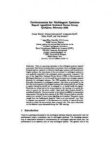
Fig. 3. Number of agent classes an A D H OC agent creates over time in contrast to the total number of known (fixed-strategy) opponents (which is increased by 40 in rounds 150, 300 and 450). As can be seen, the number of identified classes converges to the actual (four) strategies.

– “ALL C” (always cooperate), – “ALL D” (always defect), – “TIT FOR TAT” (cooperate in the first round; then play whatever the opponent played in the previous round) and – “TIT FOR TWO TATS” (cooperate initially; then, cooperate iff opponent has cooperated in the two most recent moves). Using these simple strategies served as a starting point to verify whether the A D H OC agent was capable of performing the task in principle. If A D H OC proved able to group a steadily increasing number of opponents into these four classes and to learn optimal strategies against them, this would prove that A D H OC can do the job. An important advantage of using these simple and well-studied strategies was that it is easy to verify whether the A D H OC agent is playing optimally, since optimal counter-strategies can be analytically derived. To obtain an adequate and fair performance measure for the classification heuristic, we compared the performance of the A D H OC agent to that of an agent who learns one model for every opponent it encounters (“One model per opponent”) and to that of an agent who learns a single model for all opponents (“Single model”). The results of these simulations are shown in figures 3 and 4. Plots were averaged over 100 simulations on a 10 × 10-grid. Parameter settings where: δ = 0.3, τ = 15, ρ1 = 0.6, ρ2 = 0.9, k = 80 and l = 10. 6 samples where stored for each class in order to learn opponent automata. They prove that the agent is indeed capable of identifying the existing classes, and that convergence to a set of opponent class is robust against entry of new agents into the system.

32

Reward per 100 Games

30

28

26

24

AdHoc Agent One Model per Opponent Single Model 0

5000

10000

15000 20000 Played PD Games

25000

30000

35000

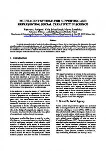
Fig. 4. Comparison of cumulative rewards between A D H OC agent, an agent that maintains one model for each opponent and an agent that has only a single model for all opponents in the same setting as above.

In terms of scalability, this is a very important result, because it means that A D H OC agents are capable of evolving a suitable set of opponent classes regardless of the size of the agent population, as long as the number of strategies employed by adversaries is limited (and in most applications, this will be reasonable to assume). A look at performance results with respect to utility reveals even more impressive results. It shows that the A D H OC agent not only does better than the “single model” agent (which is quite natural), but that it also significantly outperforms an allegedly “unboundedly rational” agent that is capable of constructing a new opponent model for each adversary! Even though the unboundedly rational agent’s performance is steadily increasing, it remains below that of the A D H OC agent even after 40000 encounters. This sheds new light on the issues discussed in section 2, because it means that designing learning algorithms in a less “individual-focused” way can even speed-up the progress in learning. In technical terms, the reason for this is easily found. The speed-up is caused by the fact that the A D H OC agent obtains much more learning data for every class model it maintains by forcing more than one agent into that model, thus being able to learn a better strategy against every class within a shorter period of time. This illustrates an aspect of learning in open systems that we might call “social complexity reduction”: the ability to adapt to adversaries quickly by virtue of creating stereotypes. If opponents can be assumed to have something in common (their strategy), learning whatever is common among them can be achieved faster if they are not granted individuality. Another issue that deserves analysis is, of course, the appropriate choice of the upper bound k for the number of possible opponent classes. Figure 5 shows a comparison between A D H OC agents that use values 10, 20, 40 and 80 for k, respectively, in terms of both number of opponent classes maintained and average reward per encounter.

35 k = 80 k = 60 k = 40 k = 30 k = 20 k = 10

Number of Opponent Classes

30

25

20

15

10

5

0 0

1000

2000

3000

4000

5000

6000

Simulations 33

32

Reward per 100 Games

31

30

29

28

27 k = 80 k = 60 k = 40 k = 30 k = 20 k = 10

26

25 0

2000

4000

6000

8000

10000

Number of Played PD Games

Fig. 5. Comparison between A D H OC agents using different k values. The upper plot shows the number of opponent classes the agents maintain, while the plot below shows the average reward per encounter. The number of opponent classes remains stable after circa 5000 rounds.

Even though there is not much difference between the time needed to converge to the optimal number of opponent classes, there seem to be huge differences with respect to payoff performance. More specifically, although a choice of k = 40 instead of k = 80 seems to have little or no impact on performance, values of 10 and 20 are certainly too small. In order to interpret this result, we have to consider two different aspects of the US-L*-A D H OC system: – The more models are maintained, the more exploration will be carried out per model in order to learn an optimal strategy against it. – The fewer models we are allowed to construct, the more “erroneous” will these models be in predicting the behaviour of adversaries that pertain to them.

The first aspect is simply due to the fact that as new classes are generated, their Q-tables have to be initialised and it takes a number of Q-value updates until a reasonably good counter-strategy is learned. On the other hand, a small upper bound on the number of classes forces us to use models that do not predict their member’s behaviours correctly, at least until a large amount of training data has been gathered. This contrasts our previous observation about the potential of creating stereotypes. Although it is certainly true that we have to trade off these two aspects against each other (both extremely high and extremely low values for k seem to be inappropriate), our results here are in favour of large values for k. This suggests that allowing some diversity during learning seems to be crucial to achieve effective learning and interaction. The second series of experiments involved simulations with societies that consist entirely of A D H OC agents. Here, unfortunately, A D H OC agents fail to evolve any useful strategy, they exhibit random behaviour throughout. The reason for this is that they have fairly random initial action selection distributions (when Q tables are not filled yet and automata un-settled). Hence, no agent can strategically adapt to the strategies of others (since they do not have a strategy, either). A slight modification to the OM method, however, suffices to produce better results. We simply add the following rule to the decision-making procedure: If the automaton of a class c is constantly modified during r consecutive games, we play some fixed strategy X for r0 games; then we return to the strategy suggested by OM (c). The intuition behind this rule can be re-phrased as follows: if an agent discovers that her opponent is not pursuing any discernible strategy whatsoever, it takes the initiative to come up with a reasonable strategy itself. In other words, she tries to become “learnable” herself in the hope that an adaptive opponent will develop some strategy that can be learned in turn. An important design issue is which strategy X to use in practice, and we investigated four different methods: 1. Use TIT FOR TAT on the grounds that it is stable and efficient in the IPD domain. 2. Use a fixed strategy that is obtained by generating an arbitrary DFA. 3. Pick that strategy from the pool of known opponent strategies C that (a) has the highest Q UALITY value, (b) provides the largest payoff. The results of these simulations are shown in figure 6. Quite clearly, the choice of TIT FOR TAT outperforms the other methods. More precisely, the A D H OC agents who have already met before will converge to the (C, C) joint action, once at least one of them has played the fixed strategy for a while (and has hence become comprehensible to its opponent). Of course, newly encountered opponents may still appear to be behaving randomly, so that sub-optimal play with those agents cannot be avoided in many situations. The superiority of TIT FOR TAT in these experiments confirms the long-lived reputation of this strategy [1], because it is known to be a very safe strategy against a variety of counter-strategies. In terms of deriving as generic method of choosing such a strategy

38

36

Reward per 100 Games

34

32

30

28

26

Tit For Tat Random Class Maximum Quality Highest Payoff

24 0

2000

4000

6000 8000 10000 Interactions (IPD Games)

12000

14000

Fig. 6. Comparison of agent performance in “A D H OC vs. A D H OC” simulations and different selection methods for the strategy chosen if the opponent exhibits random behaviour.

that does not depend on knowledge about the particular interaction problem, this is certainly not an optimal solution and is surely an issue that deserves further investigation. Still, our experiments prove that A D H OC is at least capable of “trying out” new strategies without jeopardising long-term performance, although this is certainly not optimal in decision-theoretic terms.

7 Conclusion Open systems are becoming increasingly important in real-world applications, and pose new problems for multiagent learning methods. In this paper, we have suggested a novel way of looking at the problem of learning how to interact effectively in such systems that is based on the principle of looking less at the behaviour of individual co-actors and concentrating more on learning activities that are concerned with recurring patterns of interactions that are relevant regardless of the particular opponent. We presented a framework for designing and analysing such learning algorithms based on the sociological terms of frames and framing called InFFrA and applied it to the design of a heuristic for opponent classification. A practical implementation of this heuristic in the context of a multiagent IPD scenario was used to conduct extensive empirical studies which proved the adequacy of our approach. This system called US-L*-A D H OC not only constitutes a first application of InFFrA, it also extends an existing opponent modelling method by the capability of classification, rendering this opponent modelling method usable for systems with more than just a few agents. For a particular domain of application, US-L*-A D H OC successfully addresses the problems of behavioural diversity, agent heterogeneity and agent fluctuation. It does so by allowing for different types of opponents and deriving optimal

strategies for acting towards these opponents, while at the same time coercing data of different opponents into the same model whenever possible, so that the learning efforts pay even if particular agents are never encountered again. The work presented here is only a first step toward the development of learning algorithms for open multiagent systems, and many issues remain to be resolved, out of which we can mention but a few that are directly related to our own research. One of these is the use of communication: in our experiments, the main reason for not being able to evolve cooperative interaction patterns in the “A D H OC vs. A D H OC” setting (i.e. the interesting case) unless TIT FOR TAT is used as a “fallback” strategy is the utility pressure which causes agents to use ALL D whenever in doubt (after all, it is the best strategy if we know nothing about the other’s strategy). So if agents were able to indicate what strategy they are going to play without endangering their utility performance every time, we expect the possibility for cooperation to emerge to be much bigger. Another interesting issue to explore is the application of US-L*-A D H OC to more realistic multiagent domains. Finally, a theoretical framework to analyse the trade-off between learning models of individuals vs. learning models of recurring behaviours would surely contribute to a principled development of learning algorithms for open systems.

References 1. R. Axelrod. The evolution of cooperation. Basic Books, New York, NY, 1984. 2. H. Bui, D. Kieronska, and S. Venkatesh. Learning other agents’ preferences in multiagent negotiation. In Proceedings of the Thirteenth National Conference on Artificial Intelligence, pages 114–119, Menlo Park, CA, 1996. AAAI Press. 3. D. Carmel and S. Markovitch. Learning and using opponent models in adversary search. Technical Report 9609, Technion, 1996. 4. D. Carmel and S. Markovitch. Learning models of intelligent agents. In Thirteenth National Conference on Artificial Intelligence, pages 62–67, Menlo Park, CA, 1996. AAAI Press/MIT Press. 5. C. Claus and C. Boutilier. The dynamics of reinforcement learning in cooperative multiagent systems. In Collected Papers from the AAAI-97 Workshop on Multiagent Learning, pages 13–18. AAAI, 1997. 6. Y. Freund, M. Kearns, Y. Mansour, D. Ron, R. Rubinfeld, and R. E. Shapire. Efficient Algorithms for Learning to Play Repeated Games Against Computationally Bounded Adversaries. In 36th Annual Symposium on Foundations of Computer Science (FOCS’95), pages 332–343, Los Alamitos, CA, 1995. IEEE Computer Society Press. 7. D. Fudenberg and J. Tirole. Game Theory. The MIT Press, Cambridge, MA, 1991. 8. L. Gasser. Social conceptions of knowledge and action: DAI foundations and open systems semantics. Artificial Intelligence, 47:107–138, 1991. 9. E. Goffman. Frame Analysis: An Essay on the Organisation of Experience. Harper and Row, New York, NY, 1974. Reprinted 1990 by Northeastern University Press. 10. C. Hewitt. Open information sytems semantics for distributed artificial intelligence. Artificial Intelligence, 47:79–106, 1991. 11. R. D. Luce and H. Raiffa. Games and Decisions. John Wiley & Sons, New York, NY, 1957. 12. T. Mitchell. Machine Learning. McGraw-Hill, New York, 1997. 13. A. S. Rao and M. P. Georgeff. BDI agents: From theory to practice. In Proceedings of the First International Conference on Multi-Agent Systems (ICMAS-95), pages 312–319, 1995.

14. M. Rovatsos. Interaction frames for artificial agents. Technical Report Research Report FKI244-01, AI/Cognition Group, Department of Informatics, Technical University of Munich, 2001. 15. M. Rovatsos and J. Lind. Hierarchical common-sense interaction learning. In E. H. Durfee, editor, Proceedings of the Fifth International Conference on Multi-Agent Systems (ICMAS00), Boston, MA, 2000. IEEE Press. 16. M. Rovatsos, G. Weiß, and M. Wolf. An Approach to the Analysis and Design of Multiagent Systems based on Interaction Frames. In M. Gini, T. Ishida, C. Castelfranchi, and W. L. Johnson, editors, Proceedings of the First International Joint Conference on Autonomous Agents and Multiagent Systems (AAMAS’02), Bologna, Italy, 2002. ACM Press. 17. J. M. Vidal and E. H. Durfee. Agents learning about agents: A framework and analysis. In Collected papers from AAAI-97 workshop on Multiagent Learning, pages 71–76. AAAI, 1997. 18. C. Watkins and P. Dayan. Q-learning. Machine Learning, 8:279–292, 1992. 19. G. Weiß, editor. Multiagent Systems. A Modern Approach to Distributed Artificial Intelligence. The MIT Press, Cambridge, MA, 1999.