Multidimensional data modeling for location-based services

The VLDB Journal (2004) 13: 1–21 / Digital Object Identifier (DOI) 10.1007/s00778-003-0091-3 The VLDB Journal, Volume 13, Number 1, pp 1-21, January 2004. URL: http://www.springerlink.com/link.asp?id=146e1mfw8wdanc39 The original publication is available at springerlink.com Copyright © Springer-Verlag

Multidimensional data modeling for location-based services Christian S. Jensen, Augustas Kligys, Torben Bach Pedersen, Igor Timko Aalborg University, Department of Computer Science, Fredrik Bajers Vej 7E, 9220 Aalborg Øst, Denmark; e-mail: {csj,augustas,tbp,timko}@cs.auc.dk Edited by J. Veijalainen. Received: 28 September 2002 / Accepted: 5 April 2003 c Springer-Verlag 2003 Published online: August 12, 2003 –


Abstract. With the recent and continuing advances in areas such as wireless communications and positioning technologies, mobile, location-based services are becoming possible. Such services deliver location-dependent content to their users. More specifically, these services may capture the movements and requests of their users in multidimensional databases, i.e., data warehouses, and content delivery may be based on the results of complex queries on these data warehouses. Such queries aggregate detailed data in order to find useful patterns, e.g., in the interaction of a particular user with the services. The application of multidimensional technology in this context poses a range of new challenges. The specific challenge addressed here concerns the provision of an appropriate multidimensional data model. In particular, the paper extends an existing multidimensional data model and algebraic query language to accommodate spatial values that exhibit partial containment relationships instead of the total containment relationships normally assumed in multidimensional data models. Partial containment introduces imprecision in aggregation paths. The paper proposes a method for evaluating the imprecision of such paths. The paper also offers transformations of dimension hierarchies with partial containment relationships to simple hierarchies, to which existing precomputation techniques are applicable. Keywords: Location-based services – Multidimensional data – Data modeling – Partial containment

1 Introduction Several trends in hardware technologies combine to enable the deployment of mobile, location-based e-services. These trends include continued advances in the miniaturization of electronics technologies, in display devices, and in wireless communications. Other trends include the improved performance of general computing technologies and the general improvement in the performance/price ratio of electronics. Perhaps most importantly, geopositioning is becoming increasingly available and accurate. Correspondence to: I. Timko

It is expected that the coming years will witness very large quantities of wirelessly Internet-worked objects that are location-enabled and capable of movement to varying degrees. Examples of objects of interest here include consumers using Internet-enabled mobile-phone terminals and personal digital assistants, tourists carrying online and position-aware “cameras” and “wrist watches,” vehicles with computing and navigation equipment, etc. These developments pave the way to a range of qualitatively new types of Internet-based services [12]. These types of services—which either make little sense or are of limited interest in the traditional context of fixed-location, desktop computing—include the following: traffic coordination, management, and way-finding, location-aware advertising, integrated information services, e.g., tourist services, safety-related services, and location-based games that merge virtual and physical spaces. A single generic scenario may be envisioned for these location-based services. Moving service users disclose their positional information to services, which in turn use this and other information to provide specific content and functionality. The services capture the requests they receive, including their geographical origins, in a multidimensional database, i.e., a data warehouse. We note that the privacy of service users is a concern and that legislation is available that regulates this aspect (e.g., [8]). We are aware that some service providers require each customer to enter into an explicit agreement with the provider that covers the provider’s possible use of the customer’s location data. Querying the resulting data warehouse enables the services to analyze their interactions with the users, thus allowing the services to customize their interactions with the users. As a result, each user receives a service customized to the user’s specific preferences and needs and current situation. For example, the query “show the number of requests per district for user X” provides valuable information about the geographical behavior of user X. In addition, the accumulated data are used by the service providers for delayed modification of the services provided and for longer-term strategic decision making. For example, the query “show the number of requests per

2

C.S. Jensen et al.: Multidimensional data modeling for location-based services

city per quarter for the last year" gives information about the changes in service use for different cities over time. A data warehouse [1,15,25] is a large repository that organizes data specifically for analytical purposes by employing a multidimensional view of data. Multidimensional models view a central data element for the given domain, e.g., a service request, as a fact (also termed a cell), which is uniquely defined by a combination of dimension values, each of which stems from one of a number of hierarchically organized dimensions. Typical dimensions are the location from which the request originates, the profile of the user that has issued the request, and the time of the request. Dimensions are organized as hierarchies of levels, also termed categories. For example, the time dimension may have Day, Week, Month, Quarter, and Year levels. The multidimensional view is particularly well suited for complex data analyses, which include data aggregation [25], i.e., the counting of facts that are characterized by specific values from the dimensions. Typical operations on multidimensional data warehouses use the dimension hierarchies to dynamically change the level of detail in order to gain an understanding of a particular phenomenon. If more detail is desired, e.g., to understand why the number of requests dropped sharply in Q4 2002, a “drill down” is performed, where numbers of requests per month are used in place of numbers of requests per quarter. If the opposite is true, i.e., less detail is desired in order to get a better overview, a “roll up” is performed. This means that it is crucial for multidimensional data warehouses to have well-designed dimension hierarchies that capture the useful levels of detail. We assume this kind of data analysis in our scenario. The scenario is realistic. For example, the Danish company Euman A/S [7] has developed and deployed a service delivery system capable of providing location-based services. Although the current object-relational database underlying the system is not optimized for complex data analyses, the database contains data, e.g., data on geo-referenced transportation infrastructure, that can be used to implement a multidimensional data warehouse. This in turn enables complex multidimensional analyses of the interactions among the services delivered by the system and the users. The scenario entails the capture of spatial data in a multidimensional data warehouse. This poses new challenges. For example, an appropriate data model should support irregular, so-called nonnormalized, dimension hierarchies [26] where the hierarchies are not balanced trees. Next, while dimension values in conventional multidimensional data models either are disjoint or exhibit total containment relationships, partial containment is prevalent in spatial data. For example, a roadway that extends from a city into a rural area is only partially contained in the city. Thus, partial containments between dimension values, i.e., location values such as roadways and cities, must be supported by the data model. The inclusion of advanced modeling facilities in a data model should not preclude the provision of an efficient implementation of the data model. In a multidimensional context, this implies that conventional preaggregation techniques [32] should remain applicable. This paper first analyzes the mobile e-service application domain, formulating requirements to a data model. It then presents a new multidimensional data model with an accom-

panying algebraic query language that arguably meets the requirements. Notably, the model supports nonnormalized hierarchies and partial containment. Partial containment, together with its transitivity property, is the key new aspect of the model, and the paper treats this topic in detail. Partial containment introduces additional imprecision in aggregation paths. Because it is important to be able to evaluate the imprecision of a path (e.g., for choosing the most precise one), the paper offers a path imprecision evaluation method. Practical preaggregation, i.e., precomputation of select aggregate results that can be reused to obtain other aggregates, is a technique that is essential for efficiently implementing any multidimensional data model, including the one proposed here. We thus propose algorithms for making its dimension hierarchies onto, covering, and aggregation strict. This enables the application of standard preaggregation techniques in an implementation of the model. This paper is a revised and substantially extended version of an earlier conference paper [13]. In particular, the contents of Sects. 4.7, 5, 6, 7, and the appendix are entirely new. The remainder of the paper is structured as follows. Section 2 discusses related work. Section 3 describes key requirements of a multidimensional data model for location-based services, and Sect. 4 then presents a data model that aims to satisfy those requirements. Section 5 completes the description of the model by defining its algebraic query language. Section 6 presents the method for evaluating the imprecision of an aggregation path. Section 7 provides an overview of the algorithms for normalizing dimension hierarchies. Section 8 concludes and points to future work. The appendix provides the details of the normalization algorithms. The paper can be read and understood without reading the appendix. 2 Related work In the domain of spatial data modeling, most related scientific and industrial work is dedicated to object-relational extensions of SQL. In particular, Egenhofer [6] proposed a spatial model and query language that compared favorably to several related languages. A spatiotemporal model and a query language were formally defined by G¨uting et al. [10]. Dedicated designs of spatial relational algebras with formal semantics were also proposed by Scholl and Voisard [31] and Gorgano et al. [2]. As for industrial standards, the Open GIS Consortium [20] adopted a specification [19] for implementation of a spatial SQL extension, and Oracle Spatial [17] conforms to this specification. In essence, these works develop means of analyzing spatial data, given, among other things, varying relationships between spatial objects, e.g., overlapping, containment, etc. However, we believe that the object-relational view of data does not fully support complex data aggregation. In part, this is due to the lack of hierarchies. We therefore develop a multidimensional data model and algebra that are capable of capturing an advanced kind of relationship between spatial objects, i.e., partial containment relationships. Multidimensional data warehouses [1,15,25] are generally accepted as the most powerful platform for data analysis in terms of expressive power and performance. Expressive power is achieved mainly by using the multidimensional concepts of

C.S. Jensen et al.: Multidimensional data modeling for location-based services

dimensions and hierarchies. Good performance is achieved primarily by using preaggregation, i.e., storing precomputed results of aggregate queries and using these to answer new queries more efficiently. However, current multidimensional database technology does not support the complex structures needed to handle complex spatial information. To the authors’ knowledge, no other existing multidimensional data model offers built-in support for partial containment hierarchies. This deficiency is also suggested by surveys of multidimensional data models [26, 33]. However, rather than proposing an entirely new multidimensional data model and query language, the proposed model and query language extend a previously proposed multidimensional model and algebra [23,26]. The model that we extend was chosen because it is formally defined and because it compares favorably to 14 related data models [26]. The paper’s algorithms for the normalization of partial containment dimension hierarchies extend algorithms presented by Pedersen et al. [22,24] for use with the model being extended. Pedersen and Tryfona [27] propose a slightly different approach to the multidimensional modeling of spatial data. They ignore partial containment relationships among hierarchy values and instead consider spatial facts, i.e., values characterized by hierarchy values, that are two-dimensional regions. Their focus is on how to support practical preaggregation with such overlapping facts. The conceptual model underlying their work is the model being extended here. Ferri et al. [9] propose a method to couple a multidimensional data model with a Geographical Information System (GIS) to combine the strengths of these technologies. Modern GISs such as ArcInfo [14] and MapInfo [3] provide some support for complex geostatistical and spatial analysis. Currently, the systems neither directly support multidimensional data modeling nor use preaggregation. Incorporation of these features into the systems would enable complex data aggregation queries and consequently enhance analytical capabilities of the systems. As a result, it would be possible to use the systems in our scenario of customizing location-based services to users’ needs. The area of “imperfect” data has received a great deal of attention in general as well as specialized database contexts [5]. Within multidimensional databases, work has been done on irregular multidimensional data [4,15,26,29] and the associated summarizability problems [16,26,28]. However, none of these works consider partial containment dimension hierarchies. In the industrial domain, linear referencing [30] has been used quite widely for the positioning of business data, e.g., user locations and other points of interest, located along linear elements (e.g., roadways) in transportation infrastructures. For example, Oracle Spatial [17] offers support for linear referencing. In addition, a generic data model [18] has been recommended for the capture of different aspects of entire transportation infrastructures and related business data. By applying the multidimensional view on linearly referenced data, we would enable complex aggregation queries on this kind of business data. In order to achieve this, it is necessary that a multidimensional model provide support for nonnormalized partial containment hierarchies. For this reason, we believe that our model, which supports hierarchies of this type, could serve as a basis for complex analysis of linearly referenced data.

3

Finally, the World Wide Web Consortium [35] has recently published a draft specification [34] of an XML-based language for describing location information. In our scenario, that language could facilitate data exchange.

3 Usage scenario and requirements We introduce a prototypical usage scenario for a multidimensional database in the context of location-based services, and we use this scenario to illustrate important requirements to a multidimensional data model. The scenario is also used for exemplification throughout the paper.

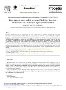
3.1 Usage scenario In our prototypical usage scenario, a user issues a service request that is characterized by a combination of values including values that capture the time and date of the request, the profile of the user, and the location from which the request originates. The ER diagram in Fig. 1 describes location values that may be used for capturing the origins of service requests as well as location values that may prove useful in analyses of service requests that involve the origins of the requests. The meanings of most of the entity types found in the diagram follow from the names of the types, though there are some exceptions, namely, the entity type IP Address represents fixed IP addresses, e.g., those of office or home desktop computers, the type Cell represents wireless network cells, the type District represents city districts, and the type Roadway represents all types of roads. The schema is meant to illustrate certain problematic properties of locations, such as partial containment hierarchies, while still maintaining simplicity. The schema is not meant to capture all aspects of locations. For example, generic international locations or locations in oceans are not handled. For information on how to model international locations, we refer to the literature [15]. The diagram uses its naming convention to distinguish between two different types of binary relationships between entities, namely, full and partial containment relationships among the spatial extents of the related entities. In the diagram, an “F” in a relationship name indicates a total, or full, containment relationship type, and a “P” indicates that only partial containment may be assumed. For example, consider the relationship type co-F-ro between entity types Coordinate and Roadway, and consider roP-di, which relates Roadway and District. The meaning is that a coordinate is either fully contained or not contained in a roadway, which, in turn, may be fully or (only) partially contained in a district. Note that all the relationship types in the diagram are stored relationship types. For example, with the relationship types coF-ro and ro-P-di present in the diagram, the relationship type co-F-di may seem redundant. However, this third relationship type captures nonredundant information. For example, some coordinates are not contained in any roadways, but are still contained in districts.

4

C.S. Jensen et al.: Multidimensional data modeling for location-based services All locations (1,n) co-F-al IP address

(1,1) Country

(1,n)

(0,n)

pr-F-co

ip-F-pr

ip-F-ci

co-F-ip

(1,n)

(0,1)

(0,1)

(1,1)

(1,n)

(1,n)

Province (1,n) ci-F-pr (1,1)

(1,n)

(1,n)

co-F-pr

di-F-pr

(1,1)

(1,1)

City (0,n)

(1,n) (1,n)

(1,n)

ce-P-pr

ro-P-co

(1,n)

ro-P-pr

(1,n)

(1,n)

di-P-ci

ro-P-ci

co-F-ci (1,n)

(0,n) (1,n)

(1,n)

(1,n)

ce-P-ci

District

(0,1)

(1,n)

(0,n)

ro-P-di (1,n)

Cell

(0,n) Roadway

(1,n)

co-F-di

(1,n) (0,1)

co-F-ce (0,n)

ce-P-di

(0,n)

(0,1)

co-F-ro (0,1) Coordinate

The existence of a partial containment relationship type between two entity types in the case study also implies the existence of a full containment relationship type between these two entity types, as full containment is a special case of partial containment. The intuition is that if objects of one type may be partially contained in objects of another type, then some objects of the former type may also be fully contained in objects of the latter type, although fewer objects will satisfy this relationship. In a multidimensional schema, user requests will be modeled as facts and the values that characterize the user requests are organized into dimensions. For our scenario, we will have three dimensions. The TIME dimension captures the time of the user requests and has categories (levels) such as Second, Minute, and Hour. The USER dimension captures aspects of the users issuing the requests. It has categories such as Spoken Language, Personal Interest, Actual Age, and Main Occupation. The LOCATION dimension captures the (possibly changing) locations of the users when the users issue requests. Entity types in the Location ER diagram are then represented as categories in the hierarchy of categories that makes up the LOCATION dimension, and relationship types in the Location ER diagram may be represented as relationships among categories in the LOCATION dimension. It is normal practice in multidimensional modeling to include only some of

Fig. 1. Location ER diagram

the relationships found in the source data, the primary driver being to obtain hierarchies useful for roll-up/drill-down operations [15]. In Sect. 4, we illustrate how the Location ER diagram is mapped to the LOCATION dimension. In particular, the issues involved in deciding how the LOCATION dimension should be modeled are discussed in detail in Sect. 4.7. As noted above, the presented usage scenario is based on a real-world location-based service delivery system [7]. The database of this system contains the data necessary for implementing a multidimensional data warehouse. For example, the available data on geo-referenced transportation infrastructure can be used to build a LOCATION dimension. Although the available data do not directly capture containment relationships between spatial entities, they can be inferred from the data. 3.2 Data model requirements Next we discuss the requirements for a multidimensional data model that contends with our usage scenario. While the requirements are all highly relevant to our context, most of them are more general and were formulated earlier. We describe the requirements only briefly and refer to the literature for further detail [26]. Other requirements are given elsewhere [11].

C.S. Jensen et al.: Multidimensional data modeling for location-based services

1. Explicit and multiple hierarchies in dimensions Dimension values are partitioned into categories of values, and categories are related via containment relationships. For example, coordinates belong to a Coordinate category, and Coordinate is contained in Country, meaning that coordinates are contained in countries. Explicit hierarchies are highly useful in data analysis as they are used for aggregating data to the right level of detail in exploratory analyses that use roll-up/drill-down operations [25]. Support for multiple hierarchies means that multiple aggregation paths are possible. These are important for a number of reasons. The key reason is that multiple hierarchies exist naturally in much data. Another reason is that these enable better handling of the imprecision in queries caused by partial containment in dimension structures. For example, in the LOCATION dimension, we obtain a more precise result if roadways are rolled up to countries directly than if roadways are rolled up to countries through districts, cities, and provinces. 2. Partial containment We have seen that two spatial values may be not only either disjoint or have one contained in the other; they may overlap. A multidimensional data model should provide built-in support for dimensions with partial containment relationships. This will increase the modeling power of the model and enable new kinds of queries. Specifically, we will be able to perform aggregation of data along hierarchies with partial containment (e.g., districts would, though approximately, roll up to cities). 3. Nonnormalized hierarchies Situations occur naturally where a hierarchy value has more than one parent, a value has no relationship to any value in the category immediately above it in the dimension hierarchy, or a value has no relationship to any value in any category below it. For example, a roadway value may be related to several district parent values, and a city value may have no cell child values. 4. Different levels of granularity In our scenario, user requests are characterized by values drawn from the dimensions. Support for different levels of granularity enables a request to refer to other values than those in the category at the lowest level of a dimension hierarchy. For example, the position of the user may be known at the level of a coordinate (precise) or at the level of a mobile phone cell (imprecise). 5. Many-to-many relationships between facts and dimensions This requirement implies that a fact may be related to more than one value in a dimension. For example, this is useful in a situation where a request is related to more than one service user. 6. Handling of imprecision When facts are characterized by dimension values from different levels, imprecision in the data occurs. In addition, partial containment introduces imprecision. Both types of imprecision may lead to imprecise aggregate query results. In the first case, a result may be imprecise because data for a query is missing. In the second case, the transitive relationships between members of aggregation paths may become imprecise (see Sect. 6 for details), rendering the results of queries imprecise. This calls for means of handling imprecision.

5

We base our proposal for a new model on an existing data model that satisfies Requirements 1, 3, 4, and 5. Moreover, Requirement 6 is partially satisfied by the algebra associated with the preexisting model. However, Requirement 2 (partial containment) is not met by this or any other existing model. 4 Data model This section extends the existing multidimensional data model [26] to support partial containment. The section also presents properties of the new model, considers its fulfillment of the requirements, and discusses how to use it when designing dimensions. 4.1 Data model definition: dimension schemas An n-dimensional fact schema is a two-tuple S = (F, D), where F is a fact type and D = {Ti , i = 1, . . . , n} is a set of dimension types. A dimension type T is a four-tuple (CT ,
T ,
T , ⊥T ), where CT = {Cj , j = 1, . . . , k} are category types of the dimension type T , and
T is a partial order on the set CT . Next,
T is the top element of the order, meaning that ∀C ∈ CT \ {
T } (C
T
T ). Symbol ⊥T is the bottom element; the precise meaning of this will be described shortly. A function Anc : CT  2CT is defined that returns the set of immediate ancestors of a category type Cj . Function Desc : CT  2CT returns the set of immediate descendants of Cj . The relation
T captures the full containment relationships between category types. We extend the definition of a dimension type by introducing an additional relation
P T ⊆ CT × CT . This new relation captures the partial containment relationships between category types. The properties of the new relation, which are properties of a partial order, are as follows: 1. ∀C ∈ CT (C 
P T C) (antireflexivity) 2. ∀(Ci , Cj ) ∈ CT × CT P ((Ci
P T Cj ) ⇒ (Cj 
T Ci )) (antisymmetry) 3. ∀(Ci , Cj , Ck ) ∈ CT × CT × CT P P (((Ci
P T Cj ) ∧ (Cj
T Ck )) ⇒ (Ci
T Ck )) (P-to-P transitivity) Relations
T and
P T are related as follows: ∀(Ci , Cj , Ck ) ∈ CT × CT × CT P 1. ((Ci
P T Cj ) ∧ (Cj
T Ck )) ⇒ (Ci
T Ck )) (P-to-F transitivity) P 2. ((Ci
T Cj ) ∧ (Cj
P T Ck )) ⇒ (Ci
T Ck )) (F-to-P transitivity) After the extension, a dimension type T is a five-tuple: (CT ,
T ,
P T ,
T , ⊥T ) (P )

We use the notation
T to indicate the union of the two orders
T and
P T . With this notation in place we can define the meaning of ⊥T being the bottom element: (P ) ∀C ∈ CT \ {⊥T } (⊥T
T C). The functions AncP and DescP provide ancestors and descendants based on the
P T relation, and functions Anc(P ) and Desc(P ) provide ancestors and descendants based on both relations.

6

C.S. Jensen et al.: Multidimensional data modeling for location-based services

All

All

Year Language group

Interests group

Age group

Country group

Occupation group

Home country

Main occupation

Week Quarter

Spoken language

Personal interest

Actual age

Sex

Month

Day ID

Hour Full containment only Minute

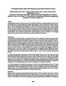
We use a fact schema to define the structure of a multidimensional data warehouse. The schema is generally capable of capturing some subset of the structure of some domain (in our scenario, the domain of a mobile e-service) at some level of abstraction. The fact schema defines facts as entities of a particular type (in our scenario, all the facts are service requests). Heterogeneous entities that characterize facts (cities, age groups, roadways, years, IP addresses, personal interests, coordinates, minutes, job categories, etc.) are organized into multiple dimensions, e.g., LOCATION and TIME dimensions. In a dimension, each type of entity has a corresponding category type (e.g., Coordinate, City, etc.). The types are organized into multiple partial and full containment hierarchies, along which the facts will be aggregated. While these hierarchies reflect some containment hierarchies of the domain (e.g., Coordinate < Cell < Province < Country <
and Coordinate < IP address < Province < Country <
), application requirements also impact the design of dimensions. With the new model fully defined, Sect. 4.7 covers dimensional database design based on the model. In essence, if we eventually wish to aggregate facts characterized by entities of type Ci (in our model, by dimension values, as defined later) with respect to entities of type Ck , then we relate these two types. Specifically, if entities of types Ci and Ck exhibit full (partial) containment relationships, we introduce the relationship Ci
T Ck (Ci
P T Ck ). The use of relations
P and
T for building hierarchies T of category types is the motivation behind defining them as partial orders. This ensures that the resulting data warehouse schema supports data aggregation. First, for a pair of category types (Ci , Cj ), the antisymmetry properties ensure that either Ci is placed higher in the hierarchy than Cj , or vice versa— both variants are not allowed at the same time. This uniquely indicates the direction of aggregation from bottom (category type ⊥T ) to top (category type
T ). Second, the transitivity enables “comparison” of category types, i.e., if Ci is lower than Cj and Cj is lower than Ck , then Ci is lower than Ck . This defines possible aggregation paths. Example 1. In Figs. 2 and 3, we present the result of applying the model to our domain. The figures depict the USER, TIME,

Second

Fig. 2. USER and TIME dimensions

All Full containment only Partial and full containment Country

Province

City

District

IP address

Roadway

Cell

Coordinate

Fig. 3. LOCATION dimension

and LOCATION dimensions. Nodes denote category types and links between nodes imply relationships between category types. Since Sect. 3 identifies three dimensions, we have a three-dimensional fact schema Scase = (Fcase , Dcase ), where Fcase = Request and the set of dimension types is Dcase = {Tloc , Tuser , Ttime }. The dimension type of the LOCATION dimension is Tloc = {Cloc,
Tloc,
P Tloc ,Call , Ccoordinate }. As a rule, the relations on set Cloc = {Ccoordinate , Croadway ,Cdistrict , Ccity , Cprovince , Ccountry , Cipaddress , Ccell , Call } are given as follows: if there exists

C.S. Jensen et al.: Multidimensional data modeling for location-based services

a relationship type of the full (partial) containment variety between entity types, the corresponding category types are P related by
Tloc (
P Tloc ) (e.g., Croadway
Tloc Cdistrict and Ccoordinate
Tloc Cprovince ). However, as noted, application requirements, e.g., support for certain roll-up and drill-down operations, also influence the design of dimensions. Thus, the LOCATION dimension models only selected aspects of the miniworld captured in the ER diagram in Fig. 1 (see Sect. 4.7 for details). (P)

We term a relationship between category types Ci
T Cj (P ) direct if it is given directly in the relation
T (without using transitivity); otherwise, the relationship is indirect. For exam(P ) ple, the relationship Roadway
T District is direct, and (P ) (P ) if also District
T City then Roadway
T City is an indirect relationship. 4.2 Data model definition: dimension instances After defining the schema level for dimensions in the data model, we proceed to define dimension instances, starting again from the prototypical data model. Given a fact schema S, a dimension of type T ∈ D is a twotuple D = (CD ,
), where CD = {Cj , j = 1, . . . , k} is a set of categories. Each category Cj has
a unique corresponding type Cj (a function T ype : CD  i CTi is defined and we write T ype(Cj ) = Cj ). A category Cj is a set of dimension values of type Cj .
The relation
is a partial order on j Cj (we henceforth
simply write Dim instead of j Cj ). The definition of the partial order is as follows. Given a pair of values (ei , ej ) ∈ Ci ×Cj such that T ype(Ci )
T T ype(Cj ), ei
ej means that ei is fully contained in ej . Dimension values of the category of type ⊥T , i.e., the “lowest” dimension values, are contained in values of other categories but do not contain anything themselves. The category of type
T has exactly one value, i.e., the “highest” value, denoted
, containing all values in the dimension. Note that the partial order on category types and the functions Anc and Desc imply a corresponding order and corresponding functions on categories. We extend the definition of a dimension by generalizing the existing partial order
on dimension values, which is capable only of expressing full containment hierarchies. Specifically, we replace
by a relation P ⊆ Dim × Dim × [0; 1]. In a triple (ei , ej , d) ∈ P , we refer to the value d as the degree of containment. With this extension, a dimension is a two-tuple D = (CD , P ). Example 2. Our LOCATION dimension is given by Dloc = (Cloc , Ploc ), where Cloc = {Coordinate, Roadway, District,City, Province, Country, IPAddress, Cell ,
} (one category for each node in Fig. 3). As reflected in the name of the new relation (P stands for “partial”), triples in the relation P define partial containment relationships between dimension values. The definition of the relation is as follows. Given a pair of values (ei , ej ) ∈ Ci ×Cj (P ) such that T ype(Ci )
T T ype(Cj ), we define (ei , ej , d) ∈ P , or simply ei
d ej , to mean that dimension value ei is

7

contained in dimension value ej so that the size of the part of ei contained in ej is larger than or equal to d times the size of ei . Intuitively, we expect that in most cases when we record a relationship in our warehouse, 0 < d < 1. To record this, it is required that T ype(Ci )
P T T ype(Cj ). In the special case where d = 1, which is defined only if T ype(Ci )
T T ype(Cj ), we say that dimension value ei is fully contained in dimension value ej . When d = 0, which requires that T ype(Ci )
P T T ype(Cj ), ei may be contained in ej . (P ) Finally, if T ype(Ci )
T T ype(Cj ), we also define ei 
ej to mean that dimension value ei is not contained in dimension value ej . In the following, we assume that ei ∈ Ci , ej ∈ Cj and ek ∈ Ck . We also assume that T ype(Ci ) = Ci , T ype(Cj ) = Cj , T ype(Ck ) = Ck and that (Ci
T Cj
T Ck ). The basic properties of the new relation are as follows. 1. Containment in all: ∀e ∈ Dim \ {
}(e
1
) Naturally, each dimension value e is fully contained in the “highest” dimension value. 2. Transitivity of full containment (f-to-f transitivity): ∀(ei , ej , ek ) ∈ Ci × Cj × Ck (((ei
1 ej ) ∧ (ej
1 ek )) ⇒ (ei
1 ek )) If ei is fully contained in ej and ej is fully contained in ek , it is natural to infer that ei is fully contained in ek . In defining the transitivity of partial containment, we employ a “safe” approach, where the idea is that we infer the relationships between dimension values with the maximum degrees of containment that hold. 3. Transitivity of partial containment: (P ) (P ) Assume that (Ci
T Cj
T Ck ). Then the following hold. ∀(ei , ej , ek ) ∈ Ci × Cj × Ck : (a) p-to-f transitivity: ∀d ∈ [0; 1)((ei
d ej ) ∧ (ej
1 ek ) ⇒ (ei
d ek )) While ek may contain the part of ei that is not in ej , the conditions of the property do not give us information on this. We infer only what we can guarantee: what is contained in ej is also contained in ek . (b) f-to-p transitivity: ∀d ∈ [0; 1)((ei
1 ej ) ∧ (ej
d ek ) ⇒ (ei
0 ek )) If ei is fully contained in ej and ej is partially contained in ek then we can only infer that at least no part of ei is contained in ek . In other words, we infer that ei may be contained in ek . (c) p-to-p transitivity: ∀(di , dj ) ∈ [0; 1) × [0; 1) ((ei
di ej ) ∧ (ej
dj ek ) ⇒ (ei
0 ek )) The reasoning follows the pattern from above: if ei is partially contained in ej and ej is also partially contained in ek , then we can only infer that ei may be contained in ek . 4.3 Building a dimension hierarchy To convey the intuition behind the definition of a dimension, we consider the construction of the hierarchy in a dimension instance, the focus being on the relation P .

8

C.S. Jensen et al.: Multidimensional data modeling for location-based services

All

1 Country

Country1 1

1

City1

City

City2 0.3

1

0.5

0.7

1

0

0 District

District2

District1

District3

1 0 0.5

1 1

0.4

0.6 Roadway

a

Roadway1

Roadway2

Roadway3

Roadway4

b

Fig. 4a,b. Schema a and instance b of a simplified LOCATION dimension

In the explanation of how we construct a dimension hierarchy, we term a relationship between dimension values ei
d ej direct if it is given explicitly in the relation P (without using transitivity); otherwise, the relationship is indirect. In short, direct relationships are used to support data aggregation from one category to any category immediately above it. In turn, indirect relationships support data aggregation from one category to any higher category. In order to exemplify the process of building dimension


hierarchies, we introduce a dimension Dloc = (CDloc , Ploc ), which is a simplified version of the LOCATION dimension Dloc . Figure 4a depicts the schema of this dimension. Based on our scenario, we assume that we have the following dimension values: coordinates Coord 1 and Coord 2, roadways Roadway1 and Roadway2, cities City1 and City2, district District1, province Province1, etc. Each of the values belongs to precisely one category (e.g., Roadway1 belongs to the Roadway category), and they are related to other values
via a dimension hierarchy given by partial order Ploc . Figure 4b then depicts an (incomplete) instance that corresponds to this schema. More specifically, the solid links between dimension values represent relationships that would be
captured explicitly in relation Ploc , i.e., direct relationships. The numbers next to the links denote containment degrees. The dotted and dashed links represent indirect, inferred relationships between dimension values. We now explain how to build a relation P while exempli
fying the process by building relation Ploc . First, we populate
Ploc with special direct relationships between dimension values that hold for every domain. Specifically, for each dimension value, e.g., Roadway1, we add Roadway1
1
to the relation. Second, we add other direct relationships, but now domain-specific. For example, if we know that District1 lies fully within City1 and that 50% of Roadway1 is in District1, then we add District1
1 City1 and Roadway1
0.5 Disctrict1 to the relation. We do not introduce zero-degree containments in this step because we assume that all relationships that exist are known to us. If we were uncertain about

some relationships, direct zero-degree containment relationships could result. Third, by applying transitivity to the relationships that we have so far, we infer new, indirect relationships. While transitivity is initially applied to the direct relationships, it is applied repeatedly until no new relationships may be inferred. We proceed to consider some examples. Using f-to-f transitivity, if Roadway2
1 District1 and District1
1 City1, we infer Roadway2
1 City1. Thus, if we know that Roadway2 is fully contained in District1 and that District1 is fully contained in City1, then we infer that Roadway2 is fully contained in City1. If Roadway1
0.5 District1 and District1
1 City1, we may use p-to-f transitivity to infer Roadway1
0.5 City1. So if we know that 50% of Roadway1 is in District1 and that District1 lies fully within City1, we infer that 50% of the roadway Roadway1 is in City1. The result can be imprecise, but we acknowledge that some part of Roadway1 lies in City1 and indicate the guaranteed percentage. As an example of using f-to-p transitivity, if Roadway3
1 District2 and District2
0.7 City2, we infer Roadway3
0 City2. This means that if we know that the roadway Roadway3 is in District2 and also that 70% of District2 is contained in City2, we can only infer that Roadway3 may be contained in City2. We may also use p-to-p transitivity: if Roadway2
0.6 District2 and District2
0.3 City1, we infer Roadway2
0 City1. In other words, we can only infer that Roadway2 may be contained in City1. To summarize, in our model, we relate two values according to full, or partial with nonzero-degree, containment if it is given that the domain entities they represent exhibit the specific relationship. We relate two values according to partial containment with zero degree if we can infer that the entities they represent may be related according to partial containment. If it is given that two entities are unrelated or if we cannot infer their relation, we do not relate the corresponding values. We note that if there are no partial containment relationships in a domain, we could still use the extended model. For category types, we then just use notation Ci
T Cj and Ci 
T Cj (full and no containment, respectively) and never use notation Ci
P T Cj (partial containment). For dimension values, we just use notation ei
1 ej and ei 
ej (full and no containment, respectively) and do not use notation ei
d ej , where d ∈ [0; 1) (partial containment). 4.4 Data model definition: facts For the formal definition of facts, we define ei 1 ej ≡ (ei
1 ej ) ∨ (ei = ej ) and Ci T Cj ≡ (Ci
T Cj ) ∨ (Ci = Cj ). Consider a set of facts F of type F and a dimension D = (CD , P ). A fact-dimension relation R is defined as R ⊆ F × Dim. In the prototypical model, a fact f ∈ F is said to be characterized by dimension value ek , written f  ek , if ∃ei ∈ Dim ((f, ei ) ∈ R ∧ ei ek ). It is required that ∀f ∈ F (∃e ∈ Dim ((f, e) ∈ R)). We extend this definition in only one respect: as a consequence of introducing partial containment, we need to use pcharacterization. We say that a fact f ∈ F is 0-characterized by dimension value ek , written f 0 ek , if ∃ei ∈ Dim

C.S. Jensen et al.: Multidimensional data modeling for location-based services

All

1 Country

Country1 1

District

City2

1

0

0.3

1

District1

Roadway1

0.7

1

Finally, a multidimensional object (MO) is a four-tuple M = (S, F, DM , RM ), where S = (F, D = {Ti , i = 1, . . . , n}) is a fact schema, F is a set of facts of type F, DM = {Di , i = 1, . . . , n} is a set of dimensions, where dimension Di is of type Ti , and where RM = {Ri , i = 1, . . . , n} is a set of fact-dimension relations such that ∀i ((f, e) ∈ Ri ⇒ ((f ∈ F ) ∧ ∃C ∈ CDi (e ∈ C))). A multidimensional object brings the different parts of the domain model together and completes the definition of the model.

E

0.5

1

0.6

District2 B 1

Roadway2

Roadway3

A

a

C

City1

City

Roadway

1

9

District3

0.4

Example 5. In our case, we can define the multidimensional object Mcase = (Scase , Frequest , Dcase , Rcase ). 4.5 Model properties

Roadway4

G

b

Fig. 5a,b. Relationships between facts and a simplified LOCATION dimension

(((f, ei ) ∈ R) ∧ (ei
d ek ) ∧ (d < 1)). In addition, we will refer to the characterization from the prototypical model as 1characterization, written f 1 ek , if ∃ei ∈ Dim (((f, ei ) ∈ R) ∧ (ei 1 ek )). Example 3. In our case study, the set of facts of type Frequest is Frequest = {A, B, C, . . .}. The fact-dimension relation between Dloc and Frequest could be denoted as Rloc . A fact-dimension relation links facts and corresponding dimension values. Each fact is related to at least one dimension value in each dimension. Characterization is propagated up along a hierarchy of dimension values. We use 1-characterization to mean that a fact is known for sure to be characterized by a dimension value, and we use 0-characterization to mean that a fact may be characterized by a dimension value. Example 4. Figure 5 illustrates characterization of facts from Frequest by values from the simplified LOCATION dimen
sion Dloc in Fig. 4. Unnumbered, solid arrows denote factdimension relationships. Numbered, dotted arrows denote propagated characterizations of facts. We link a fact to a dimension value if the domain object represented by that fact is characterized by the object represented by the dimension value. For example, if we know that request A has been issued from Roadway1, then we add the
pair (A, Roadway1) to the relation Rloc . We also infer characterizations of facts. This is analogous to inferring indirect relationships between dimension values using f-to-f and f-to-p transitivity. Specifically, we 1characterize a fact by a dimension value if the dimension value that it is linked to is fully contained in that dimension value.
So, if (G, Roadway2) ∈ Rloc and Roadway2
City1, then G 1 City1. In this case, it is natural to say that fact G is surely characterized by City1. Next, we 0-characterize a fact by a dimension value if the dimension value that it is linked to is only partially contained in that dimension value. For ex
ample, if (A, Roadway1) ∈ Rloc and Roadway1
0 City1, then A 0 City1. In this case, it is natural to say that fact A may be characterized by City1.

We proceed to define important properties of the data model. The definitions extend the ones given in the prototypical model with support for partial containment. In the definitions, we assume a multidimensional object M = (S, F, DM , RM ) and a dimension D ∈ DM . We also assume that T ype(Ci ) = Ci , T ype(Cj ) = Cj , and T ype(Ck ) = Ck . Definition 1. Given two distinct categories Ci and Cj , where Cj ∈ Anc (P ) (Ci ), we say that the mapping from Ci to Cj is onto if ∀ej ∈ Cj (∃(ei , d) ∈ Ci × [0; 1] (ei
d ej )); otherwise, it is non-onto. If all the mappings in a dimension are onto, we say that the dimension hierarchy is onto; otherwise, it is non-onto. Example 6. The mapping from Province to Country is onto because each country is partitioned into provinces. However, the mapping from IPAddress to City is non-onto because some cities have no computers (IP addresses). Thus, the hierarchy of the dimension Dloc is non-onto. The hierarchy of the Dtime dimension is onto. Definition 2. Given three distinct categories Ci , Cj , and (P ) (P ) Ck , where Ci
T Cj
T Ck , we say that the mapping from Cj to Ck is covering with respect to Ci if ∀(ei , d) ∈ Ci × [0; 1] (∀ek ∈ Ck ((ei
d ek ) ⇒ ∃(ej , di , dj ) ∈ Cj × [0; 1] × [0; 1] ((ei
di ej ) ∧ (ej
dj ek )))); otherwise, it is noncovering. If in a dimension all the mappings with respect to all the categories are covering, we say that the dimension hierarchy is covering, otherwise, it is noncovering. Example 7. Consider the categories Roadway, Province, and Country in Dloc . Each roadway going through some country also goes through a province. So the mapping from Province to Country is covering with respect to Roadway. Consider the categories Coordinate, Roadway, and District. Some coordinates do not lie on any roadway, so we map them directly to districts. This means that the mapping from Roadway to District is noncovering with respect to Coordinate. Thus, the hierarchy of the dimension Dloc is noncovering. In contrast, the hierarchy of the dimension Dtime is covering. Definition 3. Given two distinct categories Ci and Cj , where Cj ∈ Anc (P ) (Ci ), we say that the mapping from Ci to Cj is strict if ∀(ei , di1 , di2 ) ∈ Ci × [0; 1] × [0; 1] (∀(ej1 , ej2 ) ∈ Cj × Cj ((ei
di1 ej1 ) ∧ (ei
di2 ej2 ) ⇒ ((ej1 = ej2 ) ∧ (di1 = di2 )))); otherwise, it is nonstrict. If in a dimension all the mappings are strict, we say that the dimension hierarchy is strict; otherwise, it is nonstrict.

10

C.S. Jensen et al.: Multidimensional data modeling for location-based services

Example 8. The mapping from IP Address to Province is strict because an address uniquely identifies a province. But the mapping from Cell to Province is nonstrict because a cell may be shared by provinces. Thus, the hierarchy of the dimension Dloc is nonstrict. The hierarchy of the dimension Dtime is strict. Definition 4. We say that a dimension hierarchy is aggregation strict if it is strict or the following holds: if Cj ∈ Anc (P ) (Ci ) and a mapping from Ci to Cj exists that is nonstrict then Anc (P ) (Cj ) = ∅; otherwise, it is aggregation nonstrict. Example 9. Consider the categories Cell and Province. As the mapping from Cell to Province is nonstrict and Anc (P ) (P rovince) = ∅, the hierarchy of the dimension Dloc is aggregation nonstrict. The hierarchy of dimension Dtime is aggregation strict because it is strict. Definition 5. We say that a dimension hierarchy is normalized if it is onto, covering, and aggregation strict; otherwise, it is nonnormalized. We say that a multidimensional object is normalized if all its dimensions Di are normalized and ∀Ri ∈ RM (((f, e) ∈ Ri ) ⇒ (e ∈ ⊥Di )); otherwise, it is nonnormalized. Example 10. The hierarchy of the dimension Dtime is normalized because it is onto, covering, and strict. But the hierarchy of the dimension Dloc is nonnormalized because it is non-onto, noncovering, and aggregation nonstrict. Therefore, the multidimensional object Mcase is nonnormalized.

4.6 Meeting the requirements We now examine whether the requirements stated in Sect. 3.2 have been met. Explicit and multiple hierarchies are supported with the help of the partially ordered dimension types. Partial containment is supported with the help of special relations on category types and dimension values. The relation on dimension values supports nonnormalized hierarchies. Nonstrict hierarchies are captured by allowing a dimension value in a category to be related to several values in an ancestor category. Non-onto hierarchies may be built: a dimension value in a category is allowed to have no children in a descendant category. Noncovering hierarchies are also supported because a value is not required to be related to another value in an immediate parent category, i.e., a link between dimension values may “skip” one or more levels. Many-to-many relationships between facts and dimensions can be implemented by relating a fact to several dimension values in a dimension and relating a dimension value to several facts. This is allowed by the definition of factdimensional relationships. Different levels of granularity are handled: facts may map to dimension values from different categories. The combination of support in the data model for different levels of granularity of facts and partial containment of dimension values provides a basis for supporting imprecision in the data [26].

4.7 Designing dimension schemas We turn our attention to the design decisions that go into the creation of multidimensional dimension schemas. We initially consider the design context, then offer five guidelines for dimension schema design.

4.7.1 Design context The design of a multidimensional schema typically begins with the analysis of a single business process, e.g., users requesting services, and then determines the relevant facts and dimensions for this process. It is important that the dimensions be rich on contextual information that can be used for characterizing the facts. Rich dimensions enable multiple aggregations of facts and enable roll-up and drill-down operations. Supplying this rich context typically requires data from several data sources. Only information relevant to the analysis of the particular business process is captured in the multidimensional schema; much other information is omitted. For example, a multidimensional schema based on our scenario will leave out some of the relationships present in Fig. 1. We do not try to capture every aspect of the miniworld in one-multidimensional schema. A multidimensional model is not a replacement for the ER model or UML. It is beyond the scope of this paper to describe a full data warehouse design process in detail; for this, we refer to the literature [15]. Rather, we consider the design issues that are particular to the data occuring in location-based services, most notably spatial data hierarchies with partial containment relationships. We summarize the discussions into a set of general guidelines for the design of dimension schemas with such data. The insights and guidelines presented here are thus part of some complete methodology for multidimensional database design, e.g., the one described by Kimball et al. [15].

4.7.2 Dimension design guidelines Because the data model presented here allows partial containment relationships in dimensions, it generalizes existing models and offers new means of modeling dimensions. Below we explore pertinent implications of using the model for the design of dimensions. Section 3.1 describes a prototypical usage scenario for a multidimensional database in the context of a locationbased service. In particular, Fig. 1 depicts an ER diagram that presents various location values of relevance to location-based services. We proceed to consider the process of mapping the ER diagram to the LOCATION dimension shown in Fig. 3. The ER diagram captures information about containment relationships among various location entity types. Transitive relationships are not shown, and there are no explicit descriptions of hierarchies. We must build explicit hierarchies based on this diagram that enable the capture of data and the relevant analyses. For example, as a reflection of the relationship types ro-Pdi and di-P-ci in the ER diagram—and because a roadway is

C.S. Jensen et al.: Multidimensional data modeling for location-based services

typically contained in one city, so that we find it most informative to aggregate requests per roadway into requests per city— we will have a category Roadway that is below a category City in our dimension hierarchy. We identify the Coordinate category as the lowest category because its corresponding entity type is only contained in other types. The highest category has a single value, denoted
, that contains all other values. This value is very useful in analyses as we can easily express aggregation over a whole dimension. In our case, the ER diagram happens to have a corresponding entity type, but in many cases the
category is implicit and must be created specially for the multidimensional schema. We summarize this into the guideline “(1) build explicit hierarchies with top and bottom categories.” When building the LOCATION dimension, we obtain multiple hierarchies. The use of these is caused in part by the support for partial containment, so we explore this aspect in some detail. An obvious reason for introducing multiple hierarchies is that mutually exclusive hierarchies exist in the scenario. For example, the groupings of the coordinates of service requests by mobile cells and by an administrative unit such as roadways are exclusive, as one category cannot meaningfully be said to be contained in another. Therefore, the Cell category does not fit anywhere in the (main) hierarchy, Coordinate < Roadway < District < City < Province < Country <
. It is instead part of separate hierarchies, e.g., Coordinate < Cell < Province < Country <
, which skip the Roadway category. In general, building these kinds of hierarchies translates into inserting categories and corresponding relationships in the LOCATION dimension. We summarize this into the guideline “(2) introduce an additional hierarchy if a category does not fit into the existing hierarchies.” The other cases where it is necessary to build additional hierarchies are discussed next. An additional relationship may be inserted to “mend” a noncovering hierarchy. To illustrate, recall from Example 7 that it is possible for a coordinate to not lie on any roadway, while it does lie in some district. The consequence is that we cannot map all coordinates to their corresponding districts via the Roadway entity type in Fig. 1 or the Roadway category in Fig. 3. As we consider this mapping important for data analyses, we include a direct relationship from Coordinate to District in the LOCATION dimension. This relationship then creates a new path, or hierarchy, from Coordinate to
. We summarize this as follows: “(3) insert direct relationships to capture noncovering hierarchies.” Next, note that there are some relationship types from the ER diagram that do not have corresponding relationships in the dimension. For example, the ro-P-co relationship type would yield a direct relationship between the Roadway and Country categories, which is absent from the dimension. The following reasoning went into this design decision. First, in the real world, each roadway goes through a province that is part of some country, meaning that the relationship between Province and Country is covering with respect to Roadway. We are thus able to relate roadways to corresponding countries through values from the Province category – we do not depend on a direct relationship between the Roadway and the Country categories. Second, transitive partial containment relationships between dimension values are generally less precise than direct ones. However, in some situations, such as the one we are considering, maintaining a high pre-

11

cision of the degrees of containment in relationships between values of two categories may not be important. For example, a single roadway typically contributes only very little to the aggregate for a whole country, so the imprecision caused by rolling up through provinces is negligible and is preferred over creating a more complex schema. If high-precision partial containment relationships are important, we insert direct relationships. For example, had it been important that roadways roll up to countries as precisely as possible, we would add a direct relationship between Roadway and Country. This illustrates a trade-off: if one wants high precision, this comes at the cost of increasing the size and complexity of a dimension. The higher precision we want, the more direct relationships are needed. We summarize as follows: “(4) start with the relevant immediate parent-child relationships and insert direct, nonimmediate relationships if and only if high precision is desired.” Another aspect of dimension design is how to determine which category should be below which other category. While this may not be obvious in the general case, it is most often easy to decide how to relate two dimension categories. This is the case when values from one category are inherently “smaller” than those of another category. For example, since provinces are parts of countries, there is a full containment relationship from Province to Country, not the other way around. To illustrate that relationships between categories are not always obvious, consider the relationship between the District and City categories. In reality, districts exist that are contained in cities – they are termed city districts. The LOCATION dimension assumes this district type. However, there are also districts that contain cities, e.g., church districts may include several small “cities.” In addition, dimension values from two different categories can be of the same size, e.g., cities and districts are not related by containment relationships but simply overlap. One approach to addressing this problem is to divide the common District category into several categories, one for each district type, thus introducing, e.g., Church District and City District categories. The category City District is then placed below the City category, and Church District is placed above City. This approach does not contend well with large cities and city districts that contain church districts. Another approach is to allow districts of all types to belong to the unique District category, with a pair of symmetric direct relationships between the City and District categories, i.e., (P ) (P ) City
Tloc District and District
Tloc City. These relationships enable us to capture the desired relationships between district and city dimension values. For example, if city City1 and church district District1 overlap, we may include two relationships with the appropriate degrees of containment, e.g., City1
0.6 District1 and District1
0.2 City1. However, the antisymmetry property of the order on categories does not allow symmetric, direct relationships. This restriction aims to avoid inappropriate transitive relationships between dimension values. For example, without antisymmetry, in our case, by p-to-p transitivity it may be inferred that District1
0 District1, which is undefined. Also, performing this kind of roll up makes little sense. We summarize this last discussion into the last guideline: “(5) choose the hierarchical relationship between two cate-

12

C.S. Jensen et al.: Multidimensional data modeling for location-based services

All

1 Country

1

Country1 1

1 City

Country1 1

C

0.7 1

E District

Roadway

Roadway1

District3

District2

District1

B

1 0.6

Roadway2

0.6

0.4

1 Roadway3

0.9 D

Roadway4

Roadway1

District2 1

District3 0.7

Roadway2

Roadway5

A

A

a

0.8

1

District1

0.5

0.5

0.3

C City2

City1

City2

City1

1

b

Fig. 6a–c. Schema a and LOCATION dimensions of b

c 1 Mcase

and c

gories based on the most common case and such that aggregation makes the most sense.”

5 The algebra In this section, we present an algebra for the extended data model. It is based on the algebra for the prototypical model. We redefine the operators (selection, union, and aggregate formation) that need to be extended in order to support partial containment. The operators that can be taken directly from the prototypical algebra without modification include projection, rename, difference, and identity-based join, as well as derived operators such as value-based join, duplicate removal, SQL-like aggregation, star join, drill down, and roll up. For unary operators, we assume a single n-dimensional MO M = {S, F, DM , RM }, where DM = {Di , i = 1, . . . , n} and RM = {Ri , i = 1, . . . , n}. For binary operators we assume two n-dimensional MO’s M1 = (S1 , F1 , DM1 , RM1 ) and M2 = (S2 , F2 , DM2 , RM2 ), where DM1 = {Di1 , i = 1 , . . . , n}, DM2 = {Di2 , i = 1, . . . , n}, RM1 = {Ri1 , i = 1, . . . , n}, and RM2 = {Ri2 , i = 1, . . . , n}. Given a dimension Di with the set of categories
CDi = {Cj , j = 1, . . . , k}, we use the notation Dim i for j Cj . Example 11. In order to illustrate the workings of the oper1 ators, we construct two example MOs denoted by Mcase and 2 Mcase . Figure 6a depicts the schema of the LOCATION dimension of the MOs, which is a simplified version of that of Mcase . In Figs. 6b and 6c, the structure of the LOCATION di1 2 mensions of Mcase and Mcase , respectively, is presented, with numbers near the links denoting the degrees of containment. The arrows in Figs. 6b and 6c represent the fact-dimension relationships in the LOCATION dimensions. Note that facts may map directly to dimension values in nonbottom categories. The TIME and USER dimensions of the MOs are identical to the corresponding dimensions of Mcase .

2 Mcase

5.1 Selection operator The selection operator is used to select a subset of the facts in an MO based on a predicate. We first restate the definition from [26]. Given a predicate q : Dim 1 × . . . × Dim n  {true, false}, the selection operator for the prototypical mod

el, σ, is defined as: σ[q](M ) = M
= (S
, F
, DM , RM ),


where S = S, F
= {f ∈ F | ∃(e1 , . . . , en ) ∈ Dim 1 × . . . × Dim n ; ((q(e1 , . . . , en )) ∧ (f  e1 ) ∧ . . . ∧ (f  en ))},
DM
= DM ,
RM
= {Ri
, i = 1, . . . , n}, and Ri
= {(f
, e) ∈ Ri | f
∈ F
}. The selection operator for the extended model, σext , uses the new 2n-ary predicate qext : Dim 1 × . . . × Dim n × [0; 1] × . . . × [0; 1]  {true, false}. The resulting set of facts is F
= {f ∈ F | ∃(e1 , . . . , en ) ∈ Dim 1 × . . . × Dim n (∃(d1 , . . . , dn ) ∈ [0; 1] × . . . × [0; 1] ((qext (e1 , . . . , en , d1 , . . . , dn )) ∧ (f d1 e1 ) ∧ . . . ∧ (f dn en )))}. We thus restrict the set of facts to those that are characterized by dimension values where qext evaluates to true. In addition, we restrict the fact-dimension relations accordingly, while the dimensions and the fact schema stay the same. The operator supports partial containment by letting the value of the predicate depend on degrees of containment. This allows us to formulate queries that select either facts that are surely characterized by a dimension value, or facts that may be characterized by a value, or both. 1 Example 12. Suppose we want to select requests from Mcase that were surely issued from District2. In addition, the time of the requests we are interested in is July 14, 2001, and the users associated with the requests must be 21–30 years old. The predicate for the query is: (eloc = District2) ∧ ((euserage ∈ [21; 30]) ∧ (etime = [07 \14 \2001 ]) ∧ (dloc = 1) ∧ (duserage = 1) ∧ (dtime = 1). Notice that B 1 District2, so request B will be in the result.

C.S. Jensen et al.: Multidimensional data modeling for location-based services

13

2 Example 13. Suppose we want to select requests from Mcase that may have been issued from City1. Moreover, we take only nighttime requests (i.e., from 10 p.m. to 6 a.m.) into consideration. The predicate for this query may be given as follows: (eloc = City1) ∧ (etime ∈ {10 p.m., . . . , 12 p.m., . . . , 1 a.m., . . . , 6 a.m.}) ∧ (dloc = 0) ∧ (dtime = 1). Notice that A 0 City1, so the request A will be in the result.

1 Country1 1

1

C City2

City1 0.8

5.2 Union operator The union operator is used to take the union of two MOs. Consider two dimensions D1 = (CD1 ,
D1 ) and D2 = (CD2 ,
D2 ) of the same type T , where CD1 = {Cj1 , j = 1, . . . , m} and CD2 = {Cj2 , j = 1, . . . , m}. The union op
D erator on dimensions for the prototypical model, , is de
D


fined as follows: D = D D = (C ,
), where 1 2 D D
CD
= {Cj1 Cj2 , j = 1, . . . , m} and ∀(e1 , e2 ) ∈ (Dim 1 ∪ Dim 2 ) × (Dim 1 ∪ Dim 2 ) ((e1
D
e2 ) ⇔ ((e1
D1 e2 ) ∨ (e1
D2 e2 ))). In what follows, we use notation Cj

for Cj1 Cj2 . Consider two n-dimensional MOs with S1 =
S2 . The union operator on MOs , is de
for the prototypical
model,
fined as: M
= M1 M2 = (S
, F
, DM
, RM
), where

D 2
= {Di1 Di , i = S
= S1 , F
= F1
F2 , DM

1 1, . . . , n}, RM Ri2 , i = 1, . . . , n}.
= {Ri We proceed to first define an extended dimension union
D operator (denoted ext ). Consider two dimensions D1 = (CD1 , PD1 ) and D2 = (CD2 , PD2 ) of the same type T . We modify the condition for the partial order in the resulting dimension. Specifically, we require the following. 1. ∀(e1 , e2 ) ∈ (Dim 1 ∪ Dim 2 ) × (Dim 1 ∪ Dim 2 ) ((∃d ∈ [0; 1]((e1 , e2 , d) ∈ PD
) ⇔ (∃(d1 , d2 ) ∈ [0; 1] × [0; 1] (((e1 , e2 , d1 ) ∈ PD1 ) ∨ ((e1 , e2 , d2 ) ∈ PD2 )))) 2. ∀(e1 , e2 , d) ∈ PD
(((e1 , e2 ) ∈ Ci
× Cj
) ∧ (Cj
∈ Anc (P ) (Ci
))) ⇒ (∃(d1 , d2 ) ∈ [0; 1] × [0; 1] (((e1 , e2 , d1 ) ∈ PD1 ) ∨ ((e1 , e2 , d2 ) ∈ PD2 )) ∧ (d = max (d1 , d2 )))) Only the degrees of containment for the direct relationships are found using these rules. The indirect relationships between values in the resulting dimension are inferred using our transitivity rules. Stated less formally, given two MOs with common fact schemas, the union operator for the extended model takes the set union of facts and the fact-dimension
D relations. Dimensions are combined with the help of the ext operator. Specifically, given two dimensions of the same type, we perform set union on corresponding categories and build a new relation on dimension values: there exists a relationship between two dimension values if there exists a relationship between the values in the first dimension, in the second dimension, or in both. The degree of containment for a resulting relationship is determined in a natural way, namely, if two values are directly related in one of the two dimensions only, then their degree is transferred unchanged into the resulting dimension. However, if the values are directly related in both dimensions with two

0.3

1

E

1

0.6 Roadway1

District3

District2

District1 1 0.6

Roadway2

D

B 0.4

0.7

1 Roadway3

Roadway4 Roadway5

A 1 2 Fig. 7. Union of Mcase and Mcase

different degrees, then without breaking the principle of the safe approach we can return the maximum of the two as the new degree. Example 14. The LOCATION dimension of an MO obtained 1 2 by uniting Mcase and Mcase is depicted in Fig. 7. Note that some degrees of containment for the indirect relationships, e.g., Roadway1
0.6 City1, are not found in any of the original MOs and can only be inferred using the transitivity rules. 5.3 Aggregate formation operator The aggregate formation operator is used when applying aggregate functions to an MO. We first restate the definition from the prototypical model. We assume a family of aggregation functions G that “look up” the required data for the facts in the relevant fact-dimension relation, e.g., COUNT i finds its data in the fact-dimension relation Ri and counts them. In addition, the operator Group : Dim 1 × . . . × Dim n  2F is defined. The operator groups the facts characterized by the same dimension values, i.e., Group(e1 , . . . , en ) = {f | (f ∈ F ) ∧ (f  e1 ) ∧ . . . ∧ (f  en )}. Given a new (result) dimension Dn+1 of a new (result) type Tn+1 , an aggregation function g : 2F  Dim n+1 and a set of grouping categories {Ci ∈ Di , i = 1, . . . n}, the aggregate formation operator for the prototypical model, α, is defined as follows: M
= α[Dn+1 , g, C1 , . . . , Cn ](M ) =

(S
, F
, DM
, RM
), where S
= (F
, D
) F
= 2F ,
D
= {Ti
, i = 1, . . . , n} {Tn+1 }




Ti = (Ci ,
Ti , ⊥Ti ,
Ti ) Ci
= {Cij ∈ Ti | Type(Ci ) Ti Cij }

Ti =
Ti |C
, i ⊥
Ti = Type(Ci ),

Ti =
Ti F
= {Group(e1 , . . . , en ) | ((e1 , . . . , en ) ∈ C1 × . . . ×

14

C.S. Jensen et al.: Multidimensional data modeling for location-based services

Cn ) ∧ (Group(e1 , . . . , en
) = ∅)} D
= {Di
, i = 1, . . . , n} {Dn+1 },

Di
= (CD
,
D
), i i



CD
= {Cij ∈ Di | Type(Cij ) ∈ Ci } i

D
=
Di |D
i i



RM {Rn+1 }
= {Ri , i = 1, . . . , n} Ri
= {(f
, e
i ) | ∃(e1 , . . . , en ) ∈ C1 × . . . × Cn ((f
= Group(e1 , . . . , en )) ∧ (f
∈ F
) ∧ (ei = e
i )} and

Rn+1 = (e1 ,...,en )∈C1 ×...×Cn {(Group(e1 , . . . , en ), g(Group(e1 , . . . , en ))) | Group(e1 , . . . , en ) = ∅} Thus, for every combination of dimension values (e1 , . . . , en ) in the given grouping categories, the aggregation function g is applied to the set of facts characterized by (e1 , . . . , en ), and the result is placed in the new dimension. The new facts are of type sets of the argument fact type, and the argument dimension types are restricted to the category types that are greater than or equal to the types of the grouping categories. The dimension type for the result is added to the set of dimension types. The new set of facts consists of sets of the original facts, where original facts in a set share a combination of characterizing dimension values. The argument dimensions are restricted to the remaining category types, and the result dimension is added. The fact-dimension relations for the argument dimensions now link sets of facts directly to their corresponding combination of dimension values, and the fact-dimension relation for the result dimension links sets of facts to the function results for these sets. 1 Example 15. Consider the MO Mcase in Fig. 6b. Suppose we want to count the number of requests issued from different districts regardless of issue time and user information. The aggregate formation operator for the query would look as fol1 lows: α[RESULT , COUNT , District,
,
](Mcase ).

In the extended model, we have introduced p-characterization of facts, which allows us to capture imprecision in the data. This sort of imprecision must be accommodated by the aggregate formation operator. Specifically, this imprecision in data may be handled by grouping facts in different ways, i.e., by using alternative grouping operators. There are three ways of handling this, namely, by means of conservative, liberal, and weighted fact groupings. In the conservative grouping, we include only those facts in a group that are known for sure to belong to that group. We define the corresponding operator, Group c , as follows: Group c (e1 , . . . , en ) = {f | (f ∈ F ) ∧ (f 1 e1 ) ∧ . . . ∧ (f 1 en )}. Since only precise data will be used in calculations and the remaining data discarded, this kind of grouping is useful for computing a “lower bound” for a query result, in the sense that the query result contains as little data as possible. Example 16. Assume the aggregation query from Example 15. The requests B and E are guaranteed to have been issued from certain districts, while for the request A we only know that it may have been issued from the district District1. This means that the conservative grouping of the requests by districts would yield the fact groups {E} and {B} mapped to the values District1 and District2 in the LOCATION dimension,

respectively, as depicted in Fig. 8a. In this case, the count for both groups of requests would be 1, which can be seen from the result dimension in Fig. 8c. In the liberal grouping, a group is formed from the facts that are known to belong to the group as well as from those facts that might belong to that group. We define the corresponding operator, Group l , as: Group l (e1 , . . . , en ) = {f | (f ∈ F )∧(f d1 e1 )∧. . .∧(f dn en )∧(∀i ∈ {1, . . . , n}((di = 1) ∨ (di = 0)))}. Liberal grouping can be used for computing an “upper bound” for a query result, in the sense that the query result contains as much data as possible, because all the data, both precise and imprecise, are taken into consideration. Example 17. Assume the aggregation query from Example 15. The liberal grouping of the requests by districts would include the request A in a group, i.e., we would get the fact groups {A, E} and {B} mapped to the values District1 and District2 as depicted in Fig. 8b. In this case, the count for the groups would be 2 and 1, respectively, which is shown in Fig. 8d. Finally, in the weighted grouping, we gather both kinds of facts but apply a weight of membership to each fact in a group. For this kind of grouping we use the liberal grouping operator, i.e., Group w = Group l . We determine the weight of membership for a fact with the help of a function Weight : Dim 1 ×. . .×Dim n ×F  R by combining the fact’s degrees of containment. For example, the simplest way to combine the degrees is to take their product, namely, if f ∈ Group w (e1 , . . . , en ) and f d1 e1 , . . . , f dn en , then Weight simp (e1 , . . . , en , n f ) = i=1 di . Since weighted data will be used in calculations, with this kind of grouping an “average” for a query result could be computed. However, the choice of weighting function is crucial; an inadequate function may introduce additional imprecision into the query result. For example, Weight simp may sometimes be inadequate because it applies zero weights even for data that are imprecise with respect to just one dimension, i.e., ∀f ∈ Group w (e1 , . . . , en )((∃ei ∈ {e1 , . . . , en } (f 0 ei )) ⇒ (Weight simp (e1 , . . . , en , f ) = 0)). Example 18. Assume the aggregation query from Example 15 and the corresponding liberal grouping of the facts from Example 17. The function Weight simp would apply weights of membership to our facts as follows: Weight simp (District1,
,
, A) = 0 × 1 × 1 = 0, Weight simp (District1,
,
, E) = 1 × 1 × 1 = 1, Weight simp (District2,
,
, B) = 1 × 1 × 1 = 1. Thus, the weighted grouping will, unlike the liberal grouping, show that E is certain to be in District1 while A only may be in District1. This can then be exploited by the aggregation function, e.g., by counting the facts with their expected degree of membership in the group, which is 1 for E and 0.5 for A, resulting in a count for District1 of 1.5. 6 Imprecision in aggregation paths With partial containment in the model and transitivity of partial containment defined, we face the problem of how to choose the

C.S. Jensen et al.: Multidimensional data modeling for location-based services

1

1

1

1 City2

City1

City2

City1

0.7 {E}

1

15

0.7

0.3 1

1

0.3 1

District2 {B}

District3

District1

District2

{A, E}

1

District3

{B}

{B}

b

2

1

{A, E}

{B}

{E}

a

1

1

1 District1

c

d

Fig. 8a–d. LOCATION and RESULT dimensions after the query α a and c describe conservative grouping. b and d describe liberal grouping

most precise data aggregation path while processing a query, or more generally how to evaluate the level of imprecision of a path. We address these aspects next. Given a dimension D = (CD , P ), an aggregation path of D is a sequence of distinct categories such that for any element of the sequence Ci and its successor Cj , the following holds: Cj ∈ Anc (P ) (Ci ). In our case, we could define the aggregation path α = {Roadway,District, City, Province}. Two aggregation paths αi and αj are alternative aggregaj j i i i = Cfirst and Clast = Clast , where Cfirst tion paths if Cfirst j j i and Cfirst are their first elements and Clast and Clast are their last elements. So, α and αalt = {Roadway, Province} are alternative aggregation paths. An aggregation path is direct if it consists of just two elements. Thus, αalt is a direct aggregation path. Recall that we term a relationship between dimension values ei
d ej direct if it is given directly in the relation P (without using transitivity); otherwise, the relationship is indirect. Given an aggregation path β, ei ∈ Ci , and ej ∈ Cj , we say that a direct relationship ei
d ej is in the path β if Cj is the successor of Ci in β (in our case, Roadway1
0.2 District1 is a direct relationship in path α). Consider an aggregation path γ = {Cf irst , . . . , Clast } and its alternative direct aggregation path γalt . We build two sets M and Malt for γ and γalt , respectively. Both sets contain relationships ef irst
d elast , where ef irst ∈ Cf irst and elast ∈ Clast . Set M contains indirect relationships that are deduced using the transitivity property on the relationships in the path γ. Set Malt contains relationships in the path γalt . We proceed to compare the aggregation paths, for which purpose we introduce the concept of imprecision level of an aggregation path γ (denoted ILγ ). The imprecision level ILγ is evaluated by the following algorithm: (1) procedure EvaluateImprecision (2) ILγ ← 0 (3) for each (ef irst
dMalt elast ) ∈ Malt (4) where ef irst ∈ Cf irst ∧ elast ∈ Clast do (5) if (ef irst
dM elast ) ∈ M (6) then M ← M \ {(ef irst
dM elast )} (7) ILγ ← ILγ + |dMalt − dM | (8) else ILγ ← ILγ + dMalt (9) for each (ef irst
dM elast ) ∈ M do ILγ ← ILγ + dM

The algorithm distinguishes among three cases. First, if the link between two values exists in both paths (lines 6–7), the difference between the containment degrees is added to the running imprecision level total. Second, if the link exists only in the alternative path (line 8), the alternative containment degree is added. Third, for the remaining links, i.e., links existing only in the original paths, the original containment degrees are added. Note that if there is more than one link between two values in a given aggregation path, e.g., efirst
p1 elast and efirst
p2 elast , then the link with the maximum degree, i.e., efirst
max (p1 ,p2 ) elast , appears in the algorithm. The algorithm gives a high imprecision-level value if there is a large difference between the degrees of containment in the original and those in the alternative path. Note that the algorithm is meant only for choosing the best path among several alternatives, i.e., the algorithm does not provide an absolute estimate of the imprecision. This definition of imprecision level conforms to the intuitive understanding of imprecision, i.e., the greater the value of the imprecision level of a path, the more imprecise results from aggregating data along the path become. The method does not take noncovering mappings into consideration. Specifically, it ignores direct relationships that exist to accommodate noncovering hierarchies, e.g., relationships between dimension values in the Coordinate and District categories. In this case, we introduce additional imprecision, and the result of the algorithm could lead to the choice of a wrong candidate for the most precise aggregation path. Thus, we must use the ignored relationships. However, it is not reasonable to use as an alternative direct aggregation path the one that is included to accommodate noncovering hierarchies because this introduces excessive imprecision in the structure. For example, if not every coordinate is directly related to a province, δalt = {Coordinate, Province} must not be used. The proposed method is helpful in choosing aggregation paths while managing the trade-off between the speed of aggregation and the amount of preaggregation applied to the warehouse. Without preaggregation, there is no difference in speed between aggregation along a path and the alternative direct path. However, with preaggregation we can speed up aggregation along a given path considerably by precomputing some steps in it. Thus, having evaluated the imprecision level and aggregation speed (possibly with different preaggregation variants) of several alternative aggregation paths, we could choose the path with the highest speed (if we are interested in

16

C.S. Jensen et al.: Multidimensional data modeling for location-based services

speed), the path with the lowest imprecision level (if we are interested in precision), or a path that balances aggregation speed and imprecision. The applicability of the method is limited by the fact that in many cases we do not have an alternative direct aggregation path. In this situation, we can split the path according to the available paths and evaluate the level of imprecision of its subpaths. For example, in our case, we cannot use the method directly for the path  = {Coordinate, Roadway, District, City, Province, Country,
} because the path alt = {Coordinate,
} is absent. Instead, we could split  into two subpaths, 1 = {Coordinate, Roadway, District, City, Province} and 2 = {Province, Country,
}. Then 1 could be compared to 1alt (supposing every coordinate is directly related to a province) to get the imprecision level of the subpath. 7 Hierarchy transformations Using the data model described in Sect. 4, we are able to specify nonnormalized dimension hierarchies. However, such hierarchies pose problems to practical preaggregation, as will be explained shortly. In this section, we briefly present algorithms that normalize hierarchies (the algorithms are described in detail elsewhere [22, 24]) and extend the algorithms to accommodate partial containment. Due to space constraints, the details are deferred to the appendix. If a hierarchy is noncovering, then some links between dimension values skip one or more levels. Thus, at a “skipped” level some data are missing, and we cannot use aggregation results at a “skipped” level for computing aggregates at higher levels. For example, suppose a coordinate Coord 1 does not lie on any roadway, but in district District1. The mapping from category Roadway to category District is then noncovering with respect to the category Coordinate, and the level of Roadway is “skipped.” Thus, we cannot use aggregates at the Roadway level to calculate aggregate results at the District level. If a dimension hierarchy is non-onto, we are not able to reach some dimension values moving from bottom to top. Again, this means that we cannot reuse aggregates at the lowest level to compute aggregate results for the levels with “unreachable” values. For example, suppose there are no computers (IP addresses) in city City1 . The mapping from category IPAddress to category City is non-onto and City1, the dimension value of City category, is “unreachable.” Thus, we are unable to use aggregates at the Coordinate level to calculate aggregate results at the City level. Finally, if a hierarchy is nonstrict, some dimension values have multiple parents. Thus, moving from a child level to a parent level, we may count the same data several times. This means that we are unable to use aggregation results at the parent level to compute aggregates at the grandparent level. For example, suppose a roadway Roadway1 crosses districts District1 and District2, so that Roadway1 has two parent dimension values, District1 and District2, in category District. Moving from the level of Roadway to the level of District, we count aggregates for Roadway1 twice. Thus, we cannot use aggregates at the level of District to calculate aggregate results at the level of City.

A suite of hierarchy transformation algorithms remove these problems and thus enable correct use of preaggregation for nonnormalized hierarchies transparently to the user. The algorithms normalize dimension hierarchies in three steps: hierarchies are first made covering, then onto, and finally aggregation strict. Hierarchies are made covering by introducing intermediate “placeholder” values in the levels that are skipped by the original links between dimension values and by linking these values appropriately to the relevant existing dimension values (which may be placeholder values). Similarly, a hierarchy is made onto by “padding” the hierarchy downwards by inserting “dummy” child values for dimension values with no children. Aggregation strictness is achieved by “fusing” the set of parent values of a lower-level dimension value into one fused value and linking this new value to the appropriate child, parent, and grandparent values before continuing the process upwards in the hierarchy. The transformations include the rearranging of relationships between dimension values, but they do not take the partial containment relationships and their degrees of containment into account in the process. When extending the transformations, we must assign the proper degrees of containment with the relationships created during the transformations. We pose two requirements to the extended algorithms. First, full containment relationships between dimension values must be preserved. The reason is that if we guarantee that a dimension value is fully contained in another one, then this is the best we can get for the values. It would be unreasonable to eliminate or degrade such relationships. Second, as we follow the safe approach to the transitivity of containment, a new degree must be less than or equal to the corresponding old one. Example 19. The workings of the algorithms is best illustrated by an example. For the PMakeCovering algorithm, consider the transformation in Fig. 9a. Here the direct link between ek (using the example of a noncovering hierarchy in the beginning of this section, ek may correspond to District1) and ei2 (corresponding to Coord 1) is transformed by inserting a new placeholder value Cek (in our example, CDistrict1) in the intermediate category. This new value is then linked to ek and ei2 . The degree of containment of the first link is naturally 1, while the degree of the second link is inherited from the original direct link. For the PMakeOnto algorithm, consider the transformation in Fig. 9b. Here a new dummy value Lej2 (or LCity1 in our example of a non-onto hierarchy) is inserted below ej2 (City1) with a natural containment degree of 1. For the PMakeStrict algorithm, consider the transformation in Fig. 10. Here the multiple parents of value ei (corresponding to Roadway1 in our example introducing a nonstrict hierarchy) are fused into one new value e = {ej1 , . . . , ejm } (in our example, m = 2 and the fused value is {District1, District2}), which is then linked to ei and the parents ej1 , . . . , ejm (i.e., District1 and District2). To keep the figure simple, we have not shown additional values in the ei category. The degree of containment is computed to provide the highest possible degree that can still be guaranteed. See the appendix for details. The transformation algorithms described in the above example enable the use of practical preaggregation while still preserving the information about partial containment.

C.S. Jensen et al.: Multidimensional data modeling for location-based services

ek de

j

de d

ej de

j

d

Ce k ,e k

,e k

ej

e i ,e k 2

i1

ek

ek

,e k

e i ,e j

2

1

e i1

e i2

de

=1

Ce k de ,Ce =de i k

d

,e j

17

e i1

ek d

2

e j1 e i ,e j

,e k

e i2

de

j2

e i ,e j

,e k

e j2

d 1

ei

a

j 1,e k

e j1

e j2

d i2

de

e j ,e k

j 1,e k

dLe

1

ei

j 2,e j 2

=1

Le j 2

b

Fig. 9a,b. Transformations by the a PMakeCovering and b PMakeOnto algorithms

e k1 e k2 de

de j1

,e k

e k3 j 1 ,e k 2

de

e kn

...

de

j 2 ,e k 3

1

e j1

e j2 de

i

,e j

... de

i

1

,e j

2

e k1 e k2 j m,e k n

de,e

... de,e

e kn k2

de,e

de,e

k1

e jm de

i

,e j

{ej ,ej ,...,ej }=e 1

2

m

m

ei

8 Conclusions and research directions Mobile, location-based e-services promise to become a significant application domain for multidimensional modeling of spatial data. We envision that such services will store data about their interaction with the users in multidimensional data warehouses, which will be subsequently used to analyze the data in order to improve the services. This paper aims to provide better support for this application domain in multidimensional data warehouses, the focus being on data modeling and aggregation. This domain poses a number of interesting requirements to a multidimensional data model. One of them, partial containment among dimension values, is not supported by existing data models. This paper extends an existing, socalled prototypical, model that already satisfies other important requirements to also support partial containment. A key problem faced is to define transitivity of partial containment. The essence of the problem is which degree of containment to assign to an inferred relationship: if ((ei
di ej ) ∧ (ej
dj ek )) ⇒ (ei
d ek ), what is the value of d? We have provided a “safe” definition of partial containment, meaning that we deduce only those relationships that must hold. But at the same time, we try to maximize the containment degrees in inferred relationships. We feel that this is the most basic and useful approach. The paper also defines an algebra – with extended selection, union, and aggregate formation operators – that we believe serves well as a formal basis for an end-user query language for our model. Several elements of the algebraic operators reflect the support for partial containment. Specifically, the predicate for selection depends on degrees of containment as well as on dimension values. In addition, the union operator on dimension assigns proper degrees of containment to

e j1 e j2

kn j1

de,e

e jm

... j2

de,e

jm

d

e i ,e

ei

Fig. 10. Transformations by the PMakeStrict algorithm

resulting dimension values. Finally, the aggregate formation operator uses different grouping strategies. The presence of partial containment introduces imprecision in dimension hierarchies. In particular, one aggregation path from one level in a hierarchy to a higher level may be more precise than an alternative path. In order to make informed decisions on which path to choose among several alternatives, the paper provides a means of evaluating the imprecisions of paths. This allows the selection of paths based on their precisions and associated speeds of aggregation. Enabling practical preaggregation requires that dimension hierarchies be onto, covering, and aggregation strict. The paper extends existing hierarchy transformations to support partial containment. This extension satisfies the requirements that full containment relationships between dimension values be preserved and that the degrees of containment in partial containment relationships be as close to the original degrees as possible, but not higher (safe approach). It is relatively straightforward to provide transformations for making hierarchies onto and covering and at the same time retain old degrees. Incorporating support for partial containment into the transformation that makes hierarchies aggregation strict is a more complex task. We preserve full containment at the expense of degrees for partial containment relationships (some degrees reduce to “zero”). It would be of interest to study several aspects of the proposed data model further. The paper adopts a “safe” approach to inferring partial containment relationships among dimension values. Other approaches could be explored where “probable” partial relationships are inferred. Such approaches could be used together with the safe approach. In addition, it is possible to use more information when safely inferring partial containment relationships.

18

C.S. Jensen et al.: Multidimensional data modeling for location-based services

Next, with the partial containment, summarizability [27] is generally not guaranteed, even if a multidimensional object is normalized. It is of interest to determine which conditions are sufficient for summarizability with partial containment. Moreover, the extended aggregate formation operator does not handle the imprecision introduced by mapping of facts to dimension values of different granularities. It seems that the approach suggested in the literature [26] to handling this sort of imprecision can be extended to also contend with partial containment. Furthermore, it is very relevant to devise a prototype implementation of the model using an existing OLAP system [32]. Data models of existing systems do not meet all the formulated requirements. Therefore, they do not provide direct support for all the elements of our model. This raises issues related to model-to-model transformations. Finally, it is important to evaluate the applicability of the model. This could be achieved by populating a data warehouse that implements the model with the real-world spatial data and then performing experiments with the warehouse. Appropriate data on geo-referenced transportation infrastructures are currently available from a database of a location-based service delivery system developed and deployed by the Danish company Euman A/S [7].

levels or dimension hierarchies are either non-onto, noncovering, or nonstrict. Generally, preaggregation at the lowest level of a dimension does not take into consideration fact-dimension relationships at higher levels. So if all facts do not map to dimension values at the lowest level, some data are missing. This means that we cannot reuse aggregates at the lowest level to compute higher-level aggregate results. For example, suppose a user has issued a request from the roadway Roadway1. The corresponding fact is then mapped to the value Roadway1, which belongs to the category Roadway, not the lowest one. Data for the request are missing at the lowest level. We are thus unable to use aggregates at the level of the lowest category Coordinate to calculate aggregate results at the level of Roadway. With the extension for capturing partial containment introduced into the model, generally data in a normalized multidimensional object may become nonsummarizable. The proposed transitivity property infers only guaranteed (conservative) relationships between dimension levels, which means that real-world relationships exist that will be missed. In spite of this, normalization of dimension hierarchies is a first step toward achieving summarizability.

Acknowledgements. This research was supported in part by grants from the Danish National Centre for IT Research, the Nordic Academy for Advanced Study, and the Nykredit Corporation. We are thankful to the anonymous reviewers and the associate editor for comments that helped improve the presentation.

A.2 Hierarchy transformation algorithms

A Hierarchy transformation algorithms The appendix describes the hierarchy transformation approach in detail. A.1 Preaggregation and nonnormalized hierarchies To preaggregate data means to store results of aggregate queries. It is done in order to decrease the query response time of a data warehouse system. However, the results of full preaggregation, when all combinations of aggregates are precomputed, may require too much storage space, making full preaggregation impractical. Modern data warehouse systems instead use practical preaggregation, which means that only select combinations of aggregates are stored and reused later for computing other aggregates. Furthermore, it is important that we can preaggregate values at any combination of dimension levels and reuse the preaggregated values to compute higher level aggregate results. If this requirement is met, we say that our data is summarizable. In [27], it is mentioned that data captured by the model that we present in Sect. 4 (though without our extension for handling partial containment) is summarizable, if the multidimensional object for the data is normalized. So the problems with practical preaggregation occur if, in a multidimensional object, facts map to dimension values at different

We present pseudocode for the algorithms. The input to each algorithm is a set of tables RCi ,Cj ,X that specifies the relationships between dimension values in categories Ci and Cj (Cj ∈ Anc (P ) (Ci )). Column X in the table captures degrees of containment. In Figs. 9a, 9b, and 10, we illustrate the effects of the algorithms that make hierarchies covering, onto, and aggregation strict. On the left, a fragment of a dimension hierarchy is depicted, while on the right, the same fragment after the transformation is presented. When analyzing the algorithms, we do not cover in detail how the mappings are transformed (this is done elsewhere [22, 23]). Instead, we explain the extension and how the transformed hierarchies meet the formulated requirements.

A.3 Making hierarchies covering In Fig. 9a, we assume that ei1 ∈ Ci , ei2 ∈ Ci , ej ∈ Cj , Cek ∈ Cj , and ek ∈ Ck . We also assume that Ck ∈ Anc (P ) (Cj ), Ck ∈ Anc (P ) (Ci ), and Cj ∈ Anc (P ) (Ci ). Before the transformation we have: ei2
dei ,ek ek . We 2 may retain the same relationship between the values after the transformation, if for the new degrees of partial containment we let dei2 ,Cek = dei2 ,ek and dCek ,ek = 1. By using f-to-f or p-to-f transitivity (depending on the values of the degrees), we get: ((ei2
dei ,Cek Cek ) ∧ (Cek
dCek ,ek ek )) ⇒ 2 (ei2
dei ,ek ek ). Thus, the relationship ei2
dei ,ek ek 2 2 is retained by the algorithm. Obviously, the first requirement is met: if before the transformation dei2 ,ek = 1, this also holds after the transformation. The second requirement is also met: the degree dei2 ,ek never increases after the transformation (in fact, it remains the same).

C.S. Jensen et al.: Multidimensional data modeling for location-based services

Notice that after the transformation, altering the relationships between Ci , Cj , and Ck may be required. That P is, we state that T ype(Ci )
P T T ype(Cj ) if T ype(Ci )
T T ype(Ck ), and T ype(Ci )
T T ype(Cj ) if T ype(Ci )
T T ype(Ck ). By doing this we allow an arbitrary value of dei2 ,Cek . In addition, we must add the relationship T ype(Cj )
T T ype(Ck ), if it was not present before the transformation, to allow dCek ,ek = 1. (1) procedure PMakeCovering(C) (2) for each P ∈ Anc (P ) (C) do (3) begin (4) for each H ∈ Anc (P ) (C) where (P ) T ype(P )
T T ype(H) do (5) begin (6) L ← ΠC,H (RC,H,X ) \ ΠC,H (ΠC,P (RC,P,X )  ΠP,H (RP,H,X )) (7) N ← ΠH (L) (8) P ← P ∪ {M ark(h) | h ∈ N } (9) RP,H,X ← RP,H,X ∪ {(M ark(h), h, 1) | h ∈ N } (10) RC,P,X ← RC,P,X ∪ {(c, M ark(h), dc,h ) | (c, h) ∈ L ∧ (c, h, dc,h ) ∈ RC,H,X } (11) end (12) PMakeCovering(P ) (13) end

A.4 Making hierarchies onto In Fig. 9b, we assume that ei ∈ Ci , Lej2 ∈ Ci , ej1 ∈ Cj , ej2 ∈ Cj , and ek ∈ Ck . We also assume that Ck ∈ Anc (P ) (Cj ) and Cj ∈ Anc (P ) (Ci ). The transformation does not require altering the present degrees of containment. We let the completely new degree dLej2 ,ej2 = 1 (it conforms to the logic that a “placeholder” Lej2 for a value ej2 is fully contained in that value). Since no degrees are altered, the first and second requirements are met. Finally, we add the needed relationship between the categories Ci and Cj , i.e., T ype(Ci )
T T ype(Cj ). (1) procedure PMakeOnto(P ) (2) for each C ∈ Desc (P ) (P ) do (3) begin (4) N ← P \ ΠP (RC,P,X ) (5) C ← C ∪ {M ark(n) | n ∈ N } (6) RC,P,X ← RC,P,X ∪ {(M ark(n), n, 1) | n ∈ N } (7) PMakeOnto(C) (8) end

A.5 Making hierarchies aggregation strict In Fig. 10, we assume that ei ∈ Ci , ∀l ∈ {1, . . . , m}(ejl ∈ Cj ), ∀l ∈ {1, . . . , n}(ekl ∈ Ck ) and e = {ej1 , ej2 , . . . , ejm } ∈ Cjf (a category containing “fused” dimension values of Cj ). We also assume that before the transformation Ck ∈ Anc (P ) (Cj ) and Cj ∈ Anc (P ) (Ci ), but after the

19

transformation Ck ∈ Anc (P ) (Cjf ), Cj ∈ Anc (P ) (Cjf ), and Cjf ∈ Anc (P ) (Ci ). Before the transformation we have the set of relationships L = {ei
dei ,ej ejl , l = 1, . . . , m}. We would like to have l these relationships between the values with the same degrees after the transformation. But notice that in the transformed hierarchy, the relationships can be inferred only with the help of transitivity: ∀l ∈ {1, . . . , m}(((ei
dei ,e e) ∧ (e
de,ej l ejl )) ⇒ (ei
dei ,ej ejl )). The common initial condition for l each relationship in set L is: ei
dei ,e e. In general, the common condition does not allow us to retain all the old degrees of containment in the set. We deal with the situation as follows: if set L has any full containment relationships, we retain them (using f-to-f transitivity, the first step of which is to let dei ,e = 1); otherwise, we perform an approximation, which conforms to the “safe” approach, and retain the minimal degree in the set (using p-to-f transitivity, the first step of which is to let dei ,e = min({dei ,ejl , l = 1, . . . , m}). After having assigned a value to dei ,e , we perform further assignments. If we retain the full containment then for completion, we infer relationships as follows: ∀l ∈ {1, . . . , m}(((dei ,ejl = 1) ⇒ (de,ejl = 1)) ∧ ((dei ,ejl = 1) ⇒ (de,ejl = 0))). If we retain the minimal degree in the set then for completion, we must let ∀l ∈ {1, . . . , m} (de,ejl = 1). By p-to-f transitivity we then get the required result: ∀l ∈ {1, . . . , m}(ei
min({dei ,ej ,l=1,...,m}) ejl ). Nol tice that in the former case, for some relationships we get ei
1 ejl (by f-to-f transitivity), but for some relationships we cannot avoid using f-to-p transitivity, meaning that we get ei
0 ejl . This means that we do preserve full containment but miss the guaranteed degrees that were less than 1. We also need to contend with the set of relationships N = {ei
dei ,ek ekl , l = 1, . . . , n} (defined for the hierarchy prior l to the transformation). In doing so, we take into consideration that actions for set L have already been performed. Again, we would like for the transformation to retain these relationships with the same degrees. And again the relationships in the transformed hierarchy can be inferred only by transitivity (∀l ∈ {1, . . . , n}(((ei
dei ,e e) ∧ (e
de,ek ekl )) ⇒ l (ei
dei ,ek ekl ))). l Notice that the common initial condition for each relationship in set N is already given after we have dealt with the set L. Although this of course limits our capabilities, we follow the same logic that was applied in the case of set L: if set N has any full containment relationships, we retain them; otherwise, we apply a conservative approximation. We can preserve full containment because any full containment relationships in set N have degree dei ,e equal to 1 in the first condition. In this case, we partition set N into N1 and Np such that elements of set N1 are full containment relationships, while elements of set Np are partial containment relationships. We infer relationships as follows: ∀l ∈ {1, . . . , n}(((ekl ∈ N1 ) ⇒ (de,ekl = 1)) ∧ ((ekl ∈ Np ) ⇒ (de,ekl = 0))). By doing so, we retain full containment where it is present but miss guaranteed degrees that are less than 1 (analogously with the case of set L). If dei ,e is not equal to 1, the set N does not have any full containment relationships. We then perform approxi-

20

C.S. Jensen et al.: Multidimensional data modeling for location-based services

mation as follows: ∀l ∈ {1, . . . , n}((∃ejl
(ejl

dej

l


,ek

l

ekl )) ∧ ((dej
,ekl = 1) ⇒ (de,ekl = 1)) ∧ (dej
,ekl = 1) ⇒ l l (de,ekl = 0)). Thus, for some relationships in the set N , by p-to-p transitivity we get ei
0 ekl (this is true before the transformation as well) and for some relationships in L by pto-f transitivity we get ei
dei ,ek ekl (the degree is less than l that before the transformation, but still greater than zero). We see that the first and the second requirements to the procedure of inferring new degrees of containment are met. The drawback of the algorithm is that in some cases it substitutes zero degrees for nonzero ones. For example, if n = l = 2, then there are 4 degrees to work with and 16 variants for the set of degree values (each degree is allowed to be one or nonone). Therefore, there are 64 relationships. Twelve of them turn their degree from nonzero to zero. In the transformed dimension, we modify the relationships between category types as needed. If we need partial containment for the algorithm to work, we introduce such relationships. Otherwise, we only allow full containment. Specifically, we perform the modification of the relationships between category types according to the rules presented in the list below. We assume that T ype(Ci ) = Ci , T ype(Cj ) = Cj , T ype(Ck ) = Ck , and T ype(Cjf ) = Cjf . 1. (Ci
T Cj
T ∧(Cjf
T Ck )) 2. (Ci
P T Cj
T f ∧(Cj
T Ck )) 3. (Ci
T Cj
P T ∧(Cjf
P C )) T k P 4. (Ci
P T Cj
T f ∧(Cj
P T Ck ))

Ck ) ⇒ ((Ci
T Cjf ) ∧ (Cjf
T Cj ) ∧ f f P Ck ) ⇒ ((Ci
P T Cj ) ∧ (Cj
T Cj ) ∧

Ck ) ⇒ ((Ci
T Cjf ) ∧ (Cjf
T Cj ) ∧ f f P Ck ) ⇒ ((Ci
P T Cj ) ∧ (Cj
T Cj ) ∧

Notice that the pseudocode contains a new (compared to the variant in [22] and [23]) function onPath : [0 ; 1 ]  [0 ; 1 ]. The function works as follows: if ((ei
di ej ) ∧ (ej
dj ek ) then onPath(dj ) = di .

(1) procedure PMakeStrict(C) (2) for each P ∈ Anc (P ) (C) do (3) begin (4) if (∃e1 ∈ C(∃e2 , e3 ∈ P (∃d1,2 , d1,3 (e1
d1,2 e2 ∧ e1
d1,3 e3 ∧ e2 = e3 )))) ∧ Anc (P ) (P ) = ∅ (5) then begin (6) N ← CreateCategory(2P ) (7) if ∃d1,2 (d1,2 = 1) ∧ (e1 , e2 , d1,2 ) ∈ RC,P,X (8) then RC,N,X ← {(e1 , F use({e2 | (e1 , e2 , d1,2 ) ∈ RC,P,X }), 1)} (9) else RC,N,X ← {(e1 , F use({e2 | (e1 , e2 , d1,2 ) ∈ RC,P,X }), min({d1,2 | (e1 , e2 , d1,2 ) ∈ RC,P,X }))} (10) N ← ΠN (RC,N,X ) (11) RN,P,X ← {(e0 , e2 , ∅) | e0 ∈ N ∧ e2 ∈ U nf use(e0 )} (12) for each e2 ∈ U nf use(e0 ) where e0 ∈ N do (13) begin (14) if d1,0 = 1 ∧ d1,2 = 1 ∧ (e1 , e0 , d1,0 ) ∈ RC,N,X ∧ (e1 , e2 , d1,2 ) ∈ RC,P,X (15) then RN,P,X ← RN,P,X ∪ {(e0 , e2 , 0)} \ {(e0 , e2 , ∅)} (16) else RN,P,X ← RN,P,X ∪ {(e0 , e2 , 1)} \ {(e0 , e2 , ∅)} (17) end (18) Anc (P ) (C) ← Anc (P ) (C) ∪ {N } \ {P } (19) Anc (P ) (N ) ← {P } (20) for each G ∈ Anc (P ) (P ) do (21) begin (22) L ← ΠG (ΠN,P (RN,P,X )  ΠP,G (RP,G,X )) (23) RN,G,X ← {(e0 , e3 , ∅) | e0 ∈ N ∧ e3 ∈ L} (24) for each e3 ∈ L do (25) begin (26) if d1,0 = 1 ∧ (e1 , e0 , d1,0 ) ∈ RC,N,X ∧ e0 ∈ N (27) then (28) if d2,3 = 1∧d1,2 = 1∧d1,2 ∈ onP ath(d2,3 )∧e2 ∈ P (29) then RN,G,X ← RN,G,X ∪ {(e0 , e3 , 1)}\{(e0 , e3 , ∅)} (30) else RN,G,X ← RN,G,X ∪ {(e0 , e3 , 0)} \ {(e0 , e3 , ∅)} (31) else if d2,3 = 1 ∧ e2 ∈ P (32) then RN,G,X ← RN,G,X ∪{(e0 , e3 , 1)} \ {(e0 , e3 , ∅)} (33) else RN,G,X ← RN,G,X ∪{(e0 , e3 , 0)} \ {(e0 , e3 , ∅)} (34) end (35) Anc (P ) (N ) ← Anc (P ) (N ) ∪ {G} (36) Anc (P ) (P ) ← Anc (P ) (P ) \ {G} (37) end (38) PMakeStrict(N ) (39) end (40) else PMakeStrict(P ) (41) end

C.S. Jensen et al.: Multidimensional data modeling for location-based services

References 1. Blaha M (ed) (2001) Special section: data warehouses. IEEE Comput Mag 34(12):38–79 2. Gargano M, Nardelli E, Talamo M (1991) Abstract data types for the logical modeling of complex objects. Inform Sys 16(6):565–583 3. Daniel L, Loree P, Whitener A (2001) Inside MapInfo Professional. OnWord Press, Santa Fe 4. Dyreson CE (1996) Information retrieval from an incomplete data cube. In: Proc. 22nd international conference on very large databases, Bombay, 3–6 September 1996, pp 532–543 5. Dyreson CE (1997) A bibliography on uncertainty management in information systems. In: Motro A, Smets P (eds) Uncertainty management in information systems: from needs to solutions. Kluwer, Amsterdam, pp 413–458 6. Egenhofer MJ (1994) Spatial SQL: a query and presentation language. IEEE Transactions on knowledge and data engineering, 6(1):86–95 7. Euman (2003) http://www.euman.com. Current as of March 14, 2003 8. European Parliament and Council of the European Union (2002) Directive 2002/58/EC—Directive on Privacy and Electronic Communications. Available at: http://europa.eu.int/information society/topics/telecoms/regu latory/new rf/documents/l 20120020731en00370047.pdf. Current as of March 31, 2003 9. Ferri F, Pourabbas E, Rafanelli M, Ricci FL (2000) Extending geographic databases for a query language to support queries involving statistical data. In: Proc. 12th international conference on scientific and statistical database management, 26–28 July 2000, Berlin, pp 220–230 10. G¨uting RH, B¨ohlen MH, Erwig M, Jensen CS, Lorentzos NA, Schneider M, Vazirgiannis M (2000) A foundation for representing and querying moving objects. ACM Transactions on database systems, 25(1):1–42 11. Jensen CS, Pedersen TB (2001) Mobile e-services and their challenges to data warehousing. Datenbank Rundbrief 27:8– 16 12. Jensen CS (2002) Research challenges in location-enabled mservices. In: Proc. 3rd international conference on mobile data management, 8–11 January 2002, Singapore, pp 3–7 13. Jensen CS, Kligys A, Pedersen TB, Timko I (2002) Multidimensional data modeling for location-based services. In: Proc. 10th ACM international symposium on advances in geographic information systems, 8–9 November 2002, McLean,VA, pp 55– 61 14. Johnston K, Ver Hoef JM, Krivoruchko K (2001) Using ArcGIS Geostatistical Analyst. ESRI Press, Redlands, CA 15. Kimball R, Reeves L, Ross M, Thornthwaite W (1998) The data warehouse lifecycle toolkit. Wiley, New York 16. Lenz H, Shoshani A (1997) Summarizability in OLAP and statistical databases. In: Proc. 9th international conference on scientific and statistical database management, 11–13 August 1997, Olympia, WA, pp 39–48

21

17. Murray C (2002) Oracle spatial user guide and reference, Release 9.2. Oracle Corporation 18. National Cooperative Highway Research Program (1997) A generic data model for linear referencing systems. Transportation Research Board 19. Open GIS Consortium (1999) Open GIS simple features specification for SQL (Revision 1.1). Available at: http://www.opengis.org/techno/specs/99-049.pdf. Current as of March 31, 2003 20. Open GIS Consortium (2003) http://www.opengis.org. Current as of March 14, 2003 21. Open Mobile Alliance (2003) http://www.openmobilealliance.org. Current as of March 14, 2003 22. Pedersen TB, Jensen CS, Dyreson CE (1999) Extending practical pre-aggregation in on-line analytical processing. In: Proc. 25th international conference on very large databases, 7–10 September 1999, Edinburgh, pp 663–674 23. Pedersen TB (2000) Aspects of data modeling and query processing for complex multidimensional data. Ph.D. Thesis, Aalborg University, Aalborg Øst, Denmark 24. Pedersen TB, Jensen CS, Dyreson CE (2000) The TreeScape System: reuse of pre-computed aggregates over irregular OLAP hierarchies. In: Proc. 26th international conference on very large databases, Cairo, 10–14 September 2000, pp 595–598 25. Pedersen TB, Jensen CS (2001) Multidimensional database technology. IEEE Comput 34(12):40–46 26. Pedersen TB, Jensen CS, Dyreson CE (2001) A foundation for capturing and querying complex multidimensional data. Inform Sys 26(5):383–423 27. Pedersen TB, Tryfona N (2001) Pre-aggregation in spatial data warehouses. In: Proc. 7th international symposium on advances in spatial and temporal databases, Redondo Beach, CA, 12–15 July 2001, pp 460-478 28. Rafanelli M, Shoshani A (1990) STORM: a statistical object representation model. In: Proc. 5th conference on statistical and scientific database management, Charlotte, NC, 3–5 April 1990, pp 14–29 29. Rafanelli M (ed) (2002) Multidimensional databases: problems and solutions. Idea Group Publishing, Hershey, PA 30. Scarponcini P (2002) Generalized model for linear referencing in transportation. GeoInformatica 6(1):35–55 31. Scholl M, Voisard A (1989) Thematic Map Modeling. In: Abstracts of the 1st symposium on design and implementation of large spatial databases, Santa Barbara, 17–18 July 1989, pp 167–190 32. Thomsen E, Spofford G, Chase D (1999) Microsoft OLAP solutions. Wiley, New York 33. Vassiliadis P, Sellis TK (1999) A survey of logical models for OLAP databases. SIGMOD Record 28(4):64–69 34. World Wide Web Consortium (1999) POIX: Point Of Interest eXchange language specification. Available at: http://www.w3.org/TR/poix/. Current as of 31 March 2003 35. World Wide Web Consortium (2003) http://www.w3.org. Current as of 14 March 2003