Jan 1, 1995 -
SLL 78-269/AO cy 4
MULTIDITHER ADAPTIVE ALGORITHMS
J.E. Pearson, S. Hansen, M.L. Minden, and C. Yeh Hughes Research Laboratories 3011 Malibu Canyon Road Malibu,CA 90265
September 1976
Contract F30602-76-C-0022 Interim Technical Report No. 2 For Period 1 November 1975 Through 30 June 1976
Approved for public release; distribution unlimited
Prepared For DEFENSE ADVANCED RESEARCH PROJECTS AGENCY 1400 Wilson Boulevard Arlington, VA 22209
Monitored By AIR FORCE SYSTEMS COMMAND Rome Air Development Center Griffiss Air Force Base, NY 13441
PLEASE RETURN TO: D BSJECHNICAL INFORMATION CENTER BALLISTIC MISSILE DEFENSE ORGANIZATION 7100 DEFENSE PENTAGON WASHINGTON D.C. 20301-7100
U311l^
ßi
Effective Date of Contract
1 August 1975
Contract Expiration Date
31 July 1976
Amount of Contract
$190, 745,00
Contract Number
F30602-76-C-0022
Principal Investigator
J. E. Pearson (213) 456-6411, ext. 283
RADC Project Engineer
Robert F. Ogrodnik (315) 330-4306
ARPA Order No.
1279, Amendment No. 29
The views and conclusions contained in this document are those of the authors and should not be interpreted as necessarily representing the official policies, either expressed or implied, of the Defense Advanced Research Projects Agency or the U.S. Government.
19980513 103
UNCLASSIFIED SECURITY CLASSIFICATION OF THIS PAGE (Wien Data Entered)
READ INSTRUCTIONS BEFORE COMPLETING FORM
REPORT DOCUMENTATION PAGE I. REPORT NUMBER
4.
2. GOVT ACCESSION NO
TITLE (and Subtitle)
3. RECIPIENT'S CATALOG NUMBER
5.
TYPE OF REPORT ft PERIOD COVERED
Interim Tech. Report 2 1 Nov. 1975-30 June 1976
MULTIDITHER ADAPTIVE ALGORITHMS 6
PERFORMING ORG. REPORT NUMBER
8. CONTRACT OR GRANT NUMBERfs)
7. AUTHORf»;
J. E. Pearson, K. M. Brown, M. L. Minden, K. D. Price, and C. Yeh 9.
PERFORMING ORGANIZATION NAME AND ADDRESS
10.
Hughes Research Laboratories 3011 Malibu Canyon Road Malibu, CA 90265 II.
PROGRAM ELEMENT. PROJECT, TASK AREA a WORK UNIT NUMBERS
6E20; 1279, Amendment 29 12.
CONTROLLING OFFICE NAME AND ADDRESS
Defense Advanced Research Projects Agency 1400 Wilson Boulevard Arlington. VA 22209 14 MONITORING AGENCY NAME S ADDRESSr// .// Heron I Irmn ("..nlr./linii Clltice) Air Force Systems Command Rome Air Development Center Griffiss Air Force Base, NY 13441 16.
F30602-76-C-0022
REPORT DATE
Sept. 1976 13
NUMBER OF PAGES
15
SECURITY CL ASS. (ol this report)
64
UNCLASSIFIED I5n
DECL ASSIFICATION DOWNGRADING SCHEDULE
DISTRIBUTION STATEMENT (ol thi* Repi.rli
Approved for public release; distribution unlimited
17.
DISTRIBUTION STATEMENT (ol the abstract entere.! in 111.., I .' j (a n +6 n sin co n t) fn (x,' y) "
',
(2)
n=l
where the two-dimensional functions f are orthogonal over the correction aperture, a are the correction amplitudes, and 6 and co are the dither th n n amplitude and frequency for the n servo channel. For a zonal system, the functions f are the influence functions for the N deformable mirror actuators. For optical systems with circular apertures, a logical choice of an alternate orthogonal correction set is the Zernike polynomials. These functions are orthogonal over a circular aperture, and the lowest-order functions are the classical aberrations of tilt, focus, coma, etc., most of which are known to have large values in phase distortions produced by turbulence and thermal blooming. We have given the name "ZEP-COAT" to a multidither modal COAT system that uses Zernike modes. Using computer simulation codes, we have determined that only the 7 polynomials indicated with an asterisk in Table 1 are necessary for good correction in moderate thermal blooming. In determining that these 7 polynomials were the significant ones, a moderate blooming case was chosen (ptransmit ~ ^criticaP* T^e c*esired cw correction phasefront was calculated using a function-maximization routine. ' This phasefront was a
W. P. Brown, Jr., "Computer Simulation of Adaptive Optical Systems, Final Report on Contract N60921-74-C-0249, September, 1975. J. E. Pearson, et al. , "High Power, Closed Loop, Adaptive System (HICLAS) Study," Final Report on Contract N60921-76-C-0008.
13
Table 1.
Zernike Polynomials Used in ZEP-COAT Simulation 7 Z
n
Aberration Name
n
ßn"
X
Horizontal tilt
2
Y
Vertical tilt
2
*3
2R2 - 1
Refocus
1.5
*4
X2-Y2
Astigmatism
3
XY
Astigmatism
3
X(3R2 - 2)
Coma (Y-symmetry)
4
7a
Y(3R2 - 2)
Coma (X-symmetry)
4
8
X(X2 - 3Y2)
120 degree (5th order, Y-symmetry)
4
9a
Y(Y2 - 3X2)
120 degree (5th order, X-symmetry)
4
6R4 - 6R2 + 1
Spherical aberration
2.5
11
(X2 - Y2)(4R2 - 3)
Astigmatism (5th order)
5
12
XY (4R2 - 3)
Astigmatism (5th order)
5
X(10R4 - 12R2 + 3)
5th order coma (Y-symmetry)
6
Y(10R4 - 12R2 + 3)
5th order coma (X-symmetry)
6
20R6 - 30R4 + 12R2 - 1
5th-order spherical aberration
3. 5
*1 2a
5a *6
#10
"l3 14a *15
where X = -^= = R cos 6, Y = —\= = R sin 9, and R = x /2 /2
2
2 + y Si
a
These five polynomials are not used for compensating only therma 1 blooming because of the symmetries in the blooming distortions; t he transverse wind is in the X-direction (see Ref. 11). They are use d for turbulence compensation.
*Principal polynomials needed for blooming compensation. ' Relative dither amplitude fo r constant effective modulation index. T1994 14
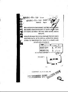
then fitted by means of an expansion using the first 44 Zernike polynomials. Table 2 lists the results of this calculation and Figure 2 shows the uncorrected and corrected beam profiles calculated for the conditions shown in Table 3.
Although there are some contributions from higher order poly-
nomials, their amplitudes are either less than 1/10 of the smallest amplitude among the 7 polynomials noted in Tables 1 and 2, or are of too high an order to be produced by a 37-element mirror.
For the planned experi-
ments, however, we will implement all 14 polynomials.
The ZEP-COAT
system can thus be used for turbulence compensation studies if so desired. Implementing a ZEP-COAT capability into the DARPA/RADC hardware is a straightforward procedure, as indicated in Figure 3. A "polynomial generator" is merely inserted between the control channels (synchronous detectors plus low-pass filters) and the drivers for the deformable mirror.
The polynomial generator is composed of several
groups of weighting matrices that distribute the error signal across the mirror in the correct manner to produce the desired polynomial spatial mode.
Since the dither and correction signals will be put onto a single
mirror for our experiments, the low-voltage dither and correction signals will be combined, put through the polynomial box, separated and separately amplified, and then recombined onto the mirror. The process is illustrated in Figure 4. A 14-channel polynomial generator is nearly complete; 37 mirror actuator drivers, each capable of ±150 V output, and a dither/correction combiner (dither injector) have already been completed. The interconnection of these units for either a zonal or a modal control system is shown in Figure 5. Because of the excessive delays in the delivery of the piezoelectric transducer (PZT) material for the deformable mirror (Section B of this chapter), the technical portion of the contract will be extended in time, but at no increase in cost, until the middle of November 1976 in order to complete the necessary thermal blooming studies.
15
-** ».
GRFv-srsi.E
t Ip»-
1*»*lli*- . » + *. ♦.
«**« . ■ *M «**' . ***♦ .
11'« - . til'i«-II«
. ♦ * 1 II
in Hi
•
GREY-SC4LE
« * 4
1 II
* li< •
Figure 2.
r.Hswjr.
TERS
A
»in R4»'l,ES
.SRKSIHF-Ob ,?7b?73t »00 .SS^SuSHOO ..H?KIM7E ton . 11 nsn2101Pt*01 . ?U»h'JSE + 0 1
,^7b?7.Utcn
.SSPSUSF+OO .«PHH17E+U0 .1 InSOOtMII .1JR136E +nt . lh57b3E tOI .l'miOttOI .?U86U5E+01 ,?7fe272E«01
CHäRA(TERS «Mi »»Mf.KS . 7C 7 1 *S^t -Oh ,H?lBa?t+on . 1 Ml 3b8E «01 ,^UnSS?t«01 .5?PMftt «01 .uioq^u «oi .149.41 Obfc +01 ,S7"S?i?RE*l'1 .hV/a JJfc+01 ,7 50hS7l- »01
.HiMRU2E«00 . lb«3b8E«01 .?Uh«Et01 . «H7JbE«0l ,U10921E. + 01 .
u
ni (X
E
o
EJJ Q
3
10
_l CL
2
(8)
where n is any number, T(x) is the gamma function, and
n
exp
[*2 + y2]n/2-[(«-ß,W] n/2
dxdy.
(9)
The quantity ß is given by
1/n vß = — v r o = (-inC m7)
(10)
Reference 4 gives the values of C sn for various choices of C m and n. For the RADC mirror, n = 1. 5 and C =0. 23, bgiving& C m ' sn 0.70. For C m =0. 20,' C sn = 0.67 and if C m =0.15, C sn =0.58. All of these values are very' substantial couplings, which may severely limit the usable COAT servo
35
bandwidth when this mirror is employed.
This is a point which we will
have to verify experimentally. The only way to reduce the servo coupling once n is fixed, Eq. (3), is to narrow the influence function, i.e., reduce Cm.
Studies conducted
on the Hughes IR&D program, however, show that n = 2. 0 minimizes C for a fixed value of C . On the other hand, reducing C m will increase sn m the interactuator ripple (surface ripple when all actuators have equal excitation). The tradeoff between ripple and Cgn as a function of Cm is shown in Figure 13. The ripple data are obtained by calculating the surface produced by a 99-actuator, hexagonal-array mirror.
Each actuator is
given a unit amplitude deflection and all actuators are assumed to have the same influence function.
The resulting surface is assumed to be a linear
superposition of all the individual actuator influence functions.
This is an
approximation, but one which should be reasonably good as long as the actuator restoring springs dominate the interactuator surface "springs" caused by the faceplate stiffness (this is expected to be the case in the RADC mirror). Note in Figure 13 that curves (b) and (c) for the ripple cross over. This implies that, for a given C , there is a value of n in Eq. (7) that minimizes the ripple. This optimum exponent is plotted in Figure 14 as a function of C . For large C , the value of n approaches 2. 0, a gausXXI xxi opt sian. For all cases, however, nQ t > 2. 0, so the RADC mirror is expected to have a larger surface ripple when excited than a mirror with a gaussian influence function. In fact, based on the data in Figures 13 and 14, it appears that the influence function on the RADC mirror is far from optimum. A value of n between 2 and 2. 5 is desirable, with Cm £ 10% so that the servo coupling will be less than 30%. The experimentally observed surface profile when two adjacent actuators are driven with the same voltage is shown in Figure 15. For reference, the individual actuator profiles are also shown. The peak-topeak surface ripple is 4. 9% of the surface deflection at one actuator location. Figure 13 predicts 8% ripple if all actuators are energized. A simple superposition of 2 actuators with the same influence function,
36
80
< LU
/U
^ < LU
fin
a.
Q.
cc O 5S
50
is
40
_l o. Q- 9: -> rr
o o o
30
tr
20
>
LU CO ii
c tn o
10 0
Cm = MECHANICAL COUPLING, %
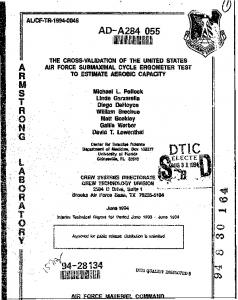
Figure 13. Servo coupling C (eq. (8)) and peak-peak ripple as a function of deformable mirror mechanical coupling, Cm (eq. (6)). Three influence function cases are shown, a "subgaussian" (n = 1.5), a gaussion (n = 2. 0), and a "supergaussion" (n = 2. 5). Further data are available in Ref. 4.
37
5554-2
cm = MECHANICAL COUPLING %
Figure 14.
Optimum value of exponent, n, in eq. (3) in order to produce minimum surface ripple.
38
5554-1
1.0 0.9
SUM OF TWO ACTUATORS
0.8 0.7 0.6 0.5 0.4
0.3 0.2 0.1 0
Figure 15.
Experimentally observed surface profile with two adjacent actuators on DARPA/RADC mirror driven with equal voltage (=30 V rms at 500 Hz). The individual actuator influence functions that produce the resultant surface are also shown.
39
IN = exp [- (r/r )1' 5], and 23% coupling, predicts a 3. 3% ripple. The difference between this value and the observed 4. 9% can be attributed to the differences between the two influence functions in Figure 14; they are not identical. C.
Irradiance Tailoring Studies The previous contract report presented some results on efforts to
find a fixed transmitter irradiance distribution that will minimize thermal blooming effects.
The basic conclusion presented there was that special laser
modes and truncated distributions have little effect on the strength of blooming at a fixed transmitted power.
In order to minimize blooming, the trans-
mitter aperture should be made as large as possible and the irradiance distribution should be made as uniform as possible. Since the time the first report was written, we have found an error in the calculations that produced Figures 7 and 10 of that report. Fortunately, the basic conclusion remains unchanged even though the quantitative output of the calculations is different. The corrected work has been accepted for publication in the Journal of the Optical Society of America, to appear in early 1977. Since the corrected results appear in that article, we present it here in its entirety as an Appendix.
40
III.
PLANS FOR THE NEXT CONTRACT PERIOD
The next phase of the contract will be devoted almost exclusively to characterizing the RADC beryllium mirror. The faceplate will be thinned to 0. 125 in. to reduce the mechanical coupling, and the unit will be polished with 19 actuators in place.
All of the data required by Amendment No. 1
to the contract will be obtained.
These data will form the substance of the
3rd interim report of the contract. In addition to completing the construction and characterization of the mirror, we will also complete the Zernike polynomial generator and set up the thermal blooming optical system. Our present plans are to use a flowing-liquid blooming medium for two reasons: (1) difficulties and safety hazards with the flowing-gas cell; (2) ease of producing substantial blooming with the limited optical power available. Previous work has indicated no signficant differences between thermal blooming produced in a gaseous or in a liquid medium.
41
APPENDIX Propagation of Laser Beams Having an On-Axis Null in the Presence of Thermal Blooming
43
PROPAGATION OF LASER BEAMS HAVING AN ON-AXIS NULL IN THE PRESENCE OF THERMAL BLOOMING* J. E. Pearson, C. Yeht, and W. P. Brown, Jr. Hughes Research Laboratories 3011 Malibu Canyon Road Malibu, California 90265 ABSTRACT The propagation of focused beams having an on-axis irradiance null is considered in the presence of thermal blooming.
Two cases are
treated: (a) beam profiles that have an irradiance zero in the beam center at the focal plane as well as the transmitter aperture; (b) beam profiles that have an on-axis irradiance null only at the transmitter. It is demonstrated that none of the beam profiles considered in case (a) has a meaningful advantage over a Gaussian beam profile. Some of the case (b) profiles do produce a larger bloomed irradiance in the focal plane, particularly when the initial intensity distribution is very uniform in its non-zero regions. Addition of a simple central obscuration to a "filled" irradiance distribution is found to have no advantage, however, for the cases considered.
*To be published in the Journal of the Optical Society of America. This work sponsored in part by the Air Force Systems Command's Rome Air Development Center, Griffiss AFB, NY. t Permanent address: Electrical Engineering Department, University of California at Los Angeles Los Angeles, California 90024 45
I.
INTRODUCTION
When an optical laser beam is propagated through an absorbing medium with a negative refractive index temperature coefficient (dn/dT < 0), the phenomenon of thermal blooming ' occurs. In the presence of thermal blooming, the propagation medium acts like a negative lens that defocuses, spreads, and distorts the optical beam. This power-dependent phenomenon can be particularly harmful when the optical system is attempting to produce maximum focal plane irradiance. It has been suggested that the use of a transmitted beam that has an annular intensity profile may provide higher focal plane irradiance in the presence of thermal blooming3 than that produced by a Gaussian beam. physical reasoning behind this suggestion is straightforward.
The
A Gaussian
intensity profile produces a quadratic refractive index variation in the medium that is minimum at the beam center where most of the optical power occurs. With an annular beam that has an on-axis null, the negative lens induced in the medium has a larger refractive index on-axis than off-axis. The result is a positive lens for light that is close to the beam axis, and this lens tends to counteract some of the off-axis negative lens beam spreading as the optical beam propagates. This article presents the results of an investigation aimed at quantifying how much thermal blooming distortions are reduced by the use of laser beam that have an on-axis intensity zero. Such beams can be produced either by apodization (truncation), or by use of laser resonators that have annular gain profiles,4 or by many unstable resonator configurations such as those used in many high energy laser devices. The investigations were performed by computer simulation of the propagation problem. The computer code5 solves the coupled differential equations that describe both the medium dynamics and the diffraction-propagation of a focused laser beam.
Convection-dominated heat transfer produced by
a transverse wind is assumed and the quantity of interest is the peak focal plane irradiance. Two types of annular or "on-axis-null" intensity profiles are treated. Section II discusses those that have an intensity zero in the beam center,
46
both in the focal plane (far-field) as well as at the transmitter (near-field) and thus are free-space propagation modes. Section III discusses those profiles that have a zero in the beam center only at the initial transmitter plane. Due to diffraction, the initial on-axis null fills in as these beams propagate so that the on-axis irradiance is not zero at the focal plane.
An
appropriate choice of the initial profile can indeed increase the maximum focal plane irradiance.
The standard of comparison in all cases is the
focal plane irradiance produced by a Gaussian beam that is truncated at the 10% intensity radius. II.
"ON-AXIS-NULL" IRRADIANCE PROFILE AT THE TRANSMITTING APERTURE (NEAR-FIELD) AND AT THE FOCAL PLANE (FAR-FIELD) In this section, we consider cases where the irradiance null in the
middle of the beam is retained as the focused beam is propagated to the target.
To first demonstrate that an appropriately chosen transmitter
irradiance distribution can indeed be focused to produce an on-axis-null focal-plane irradiance distribution, we start with a transmitter aperture 4 field given by
E(rj, Oj) = Amfm(ri) cos(m61), (m = 0, 1, 2
where A
is the maximum field magnitude, f
) ,
(1)
(r ) may be a continuous or
a discontinuous function of r , and (r^ 6.) are the transverse polar coordinates of the transmitting aperture. From Fresnel diffraction formulae, we obtain the field u at the focal plane:
U(
W
Z)
=
-WT
eX
P 1J TZ
X
o
+ y
o ) ' (2)
'
JMrl,Q1)eXp[- jg (x^+y^jjdxjdyj,
47
where z is the focal distance, \ the free-space wavelength, k = 2ir/\, (x0>yQ) are the transverse rectangular coordinates at the focal plane, and (x^Vj) are the transverse rectangular coordinates at the transmitting aperture plane.
Changing Eq. (2) into polar coordinates and carrying out the
angular integration, we find
u(r O ,
Jkz , z) = -rr—exp O J A-Z r
Jjrr
cos(mG) exp
Jkz
exp
. k J T" 2z
r
Oil ro}
\z
2 o
f
m(rl)rldrl
r cos(6 - 6 ) 1 o 1 o
2IT cos(m8 )e x o
'j
2
de.
(3)
I m (r o ),
where
I m (r o )
A mf rrr(r.) (T^r.r) 1 J m\\z lo/ r 1 dr 1
The on-axis irradiance occurs at r
(4)
=0 and is given by
[2TT
cos(m0 )T
u(0, 9o, z)
\Z
J
I2rrr(0)
(5)
Since J (0) = 0 when m 4 0, Eq. (4) indicates that I = 0 for m 4 0. An on-axis-null focal plane irradiance is thus obtained for all m 4 0. When m = 0, however, the on-axis focal plane irradiance may take on any value, including zero, depending upon the initial radial dependence of u.
48
The particular transmitter irradiance profiles that we have chosen to study are given in Eqs. (6) and (7) and are illustrated in Fig. 1.
The
truncated Gaussian beam we are using for comparison purposes is also shown in Fig. 1 and defined in Eq. (8).
Case (Il-a)
, |2 , |ul = A.
-r2/ 2 1 ^o
2
cos
8,,
= 0
Case (Il-b)
1lu
I '
< a
(6)
for r, > a 1 o
XH 7
for r
?
o'
P
= A, 2
. _ cos 6,, for b a 1 o
Case (Ill-b)
I u 12 = A.2 e "(rrrm/Po) 4
1 , for . —^ 2 p
b < r, < a o 1 o
(10)
, otherwise
Case (III-c)
, for b 1 - 1 'I1* *l|l»*. .♦«■h* **M1♦--«1*** + *1H 1 1 «*** «»tli'Mlnli*»
,
* 1««««.
, **d(BI ♦. -«iniinxt. rAC ♦ «»•Hi«*. !£.«SlttHI ♦.
******
, .
♦!)(«♦♦, .+**♦-.
•"i
• --- •
■ •-f
.---.
,la
• •
-* * -
»'llll'l.fl'* ID««»««»'!! ,|i********»< »i****irnp***»>f ill*»»»»»»*»*!!' rp**ir» xd'*** ir**iii» d'U*ft(r
. 1«*.
+nmi*. 1*111 + * til« x* tt) P
-«
2 o
o
T
(A.4)
where a is the propagation medium absorption, Fj is defined in Eq. (A-2), and F2 is given by
*a /\r2 p F2(ao/Po, p)=
|
°
°'m Jm(ß-)^x
(A-5)
and 2TTN/2 K
o
ß =
o
(A-6)
\7
We have evaluated the integral function F£ in Eq. (A-5) for each of the 7 radial f functions discussed maximum value of F2 as a function / l R? aa /D /h -= 7', rr values a /p =- 1.5£,
in the text (Eqs. (6)-(12)) to find the of the normalized parameter p. The /a = 2/3,' and ^p = 1 were used for this o 0 o Q m/*0 evaluation. Table A-l gives the results of this analysis. To obtain numerical results, we chose \= 10. 6 p-rn, Z=Z km, and PQ = 23 cm (corresponding to aQ = 35 cm). The irradiance plotted as the ordinate axes in Figs. (3) and (6) is thus given by
2
u|
=
F2 0.0592 (m+ 1) jT2-
(S.R.)PT
in units of power per square centimeter, with (S. R. ) being the strehl ratio determined by the thermal blooming computer code (S. R. = 1 for free-space propagation). For the blooming calculations, the following parameters were taken:
62