Multiple-antenna signal detection in cognitive radio ... - IEEE Xplore

IEEE ICC 2014 - Wireless Communications Symposium 1

Multiple-Antenna Signal Detection in Cognitive Radio Networks with Multiple Primary User Signals Raymond H. Y. Louie† , Matthew R. McKay† , Yang Chen∗ †

Hong Kong University of Science and Technology, Hong Kong ∗ University of Macau, Macau

Abstract—We consider multiple-antenna signal detection of primary user transmission signals by secondary user receivers in cognitive radio networks. The optimal detector is analyzed for the scenario where the number of primary user signals is no less than the number of receive antennas at the secondary users. We first derive exact expressions for the moments of the generalized likelihood ratio (GLRT) statistic, yielding approximations for the false alarm and detection probabilities. We then show that the normalized GLRT statistic converges in distribution to a Gaussian random variable when the number of antennas and observations grow large at the same rate, which is used to obtain a simple design rule for the signal detection threshold.

I. I NTRODUCTION Cognitive radio is a promising technology which can be used to improve the utilization efficiency of the radio spectrum [1], by allowing secondary user (SU) networks to co-exist with primary user (PU) networks through spectrum sharing. A key requirement is that SU transmission will not adversely affect the PUs’ performance. To achieve this, a common technique involves the SUs first detecting if at least one PU is transmitting1 . If no signals are detected, the SUs are allowed to transmit. The importance of signal detection can be seen by its inclusion in the IEEE 802.22 standard; a standard built on cognitive radio techniques [2]. Due to the importance of signal detection, a number of optimal signal detection tests have been proposed to detect PU transmission when there are multiple receive antennas at the SUs (see e.g., [3]). Optimality is typically considered in the Neyman Pearson sense, which involves comparing the generalized likelihood ratio (GLR) to a user-designed detection threshold. The GLR can be used to determine the false alarm probability and detection probability, which can then be subsequently used to design the threshold. The particular form of the GLR is dependent on the number of PU transmission signals, and whether noise and/or channel information is known at the SU receiver performing the signal detection. A reasonable scenario is to assume that nothing is known at the SU receiver, i.e., no noise and channel information are known. For this scenario, the false alarm and detection probability have been analyzed when there is only one PU signal (see e.g., [3, 4]). However, for next generation systems, scenarios exist where the number of PU signals is no less than the number of receive antennas. This may occur, for

example, in systems where spatial multiplexing techniques are employed, or where there are simultaneously transmitting PUs. For these scenarios, an exact expression for the false alarm probability and detection probability were derived in [5] when there are two receive antennas. For more general scenarios with arbitrary number of receive antennas and observations, [6] conducted Monte Carlo simulations while [7] [8, pp. 230] derived infinite series expansions. However, the expressions in [7] involved complicated zonal polynomials or Meijer-G functions which are hard to compute, while the false alarm probability expression in [8, pp. 230] was not amenable to analysis. For the same general scenario, an approximation was considered in [5], however, the approximation was only justified for the false alarm probability, and only then for a very small number of antennas. In this paper, we derive accurate easy-to-compute approximations for the false alarm and detection probabilities when there are an arbitrary number of receive antennas and observations. This is facilitated by an expression for the moments of the GLR test (GLRT) statistic which we derive. We also consider the scenario where the number of receive antennas and observations are large and of similar order. For this scenario, we show that the GLRT statistic converges in distribution to a Gaussian random variable, which facilitates a simple design rule to choose a detection threshold which can accurately achieve a desired false alarm probability. This detection threshold was also found to result in a high detection probability for different practical scenarios. Note that the performance of the GLR detector has been previously shown to perform better than other detectors in many practical scenarios [5], and thus we do not consider such comparisons in this paper. II. P ROBLEM S TATEMENT Consider a wireless communications system where a SU receiver equipped with n antennas is tasked with determining if PU transmission signals are present from m observation independent and identically distributed sample vectors x1 , . . . , xm , where2 x = CN n,1 (0n,1 , R) for = 1, . . . , m, and R is a n × n population covariance matrix. The th sample vector x for this hypothesis testing problem can be modeled as

The work of R. H. Y. Louie and M. R. McKay was supported by research grant SBI11EG15. The work of R. H. Y. Louie was also supported by HKUST research grant IGN13EG02. 1 This is also referred to as “spectrum sensing” in cognitive radio literature.

978-1-4799-2003-7/14/$31.00 ©2014 IEEE

4951

H0 : H1 : 20

p,q

x = n

no signal present

x = Hs + n

signals present

denotes the p × q matrix of all zeroes.

(1)

IEEE ICC 2014 - Wireless Communications Symposium

where n ∼ CN n,1 (0n,1 , In N0 ) denotes additive white Gausk sian noise variance N0 , s ∈ C is the signal vector with † n×k with E s s = In , H ∈ C is the channel matrix from the PUs to the SU detector, which is assumed to be constant during the m observation time periods, and k is the number of PU transmission signals. Note that unless otherwise specified, the results in this paper do not assume a specific distribution for H. Thus, for example, our results can account for each PU transmission signal having different transmit power. We assume that H, k and N0 are unknown at the detector, and that HH† is of full rank, i.e., k ≥ n. The latter condition can correspond to the scenario where there are at least n single-antenna PU transmitters, or if there is at least one PU transmitter equipped with at least n antennas which is utilized for spatial multiplexing. The detection problem in (1) is thus equivalent to testing if the population covariance matrix R is one of two structures: H0 :

R = In N 0

H1 :

R = HH† + In N0

A. False Alarm and Detection Probability To evaluate the performance of the GLRT statistic (7), we consider the false alarm and the detection probability. The false alarm probability is the probability that H1 is chosen given H0 is the true hypothesis, defined as Δ

Δ

W0 =

signals present .

Then the GLR, used for determining H0 or H1 , admits max+ f x1 , . . . , xn N0 N0 ∈R L= max f x 1 , . . . , x n N 0 , H

Δ

PD (η) = Pr (W1 > η) = 1 − FW1 (η)

Δ

W1 =

1 ≷H H0 η

Tr(XX† ) n 1 det(XX† ) n

,

X ∼ CN n,m 0n,m , HH† + In N0 (12)

and FW1 (η) denotes the c.d.f. of W1 . Note that increasing the detection threshold η decreases the false alarm probability but also decreases the detection probability. Finally, observe that to obtain the probability of false alarm and detection, the c.d.fs. of W0 and W1 are required respectively.

(4)

(5)

III. C. D . F. OF W0 AND W1 : NON - ASYMPTOTIC APPROXIMATE ANALYSIS

In this section, we derive expressions for the c.d.f. of W0 and W1 for arbitrary n and m. To do this, we first present closed-form expressions for the moments of W1 : Theorem 1. The pth (p ∈ Z+ ) moment of W1 , for p < n(m − n + 1), is given by p

n n−1 p! i=1 yin Γ m − n + 1 − np + j p E [W1 ] = np Γ (m − n + 1 + j) j=0

n

Γ m − np + ki × (13)

Γ(ki + 1)Γ m − np yiki k1 +...+kn =p i=1

is the corresponding likelihood function under hypothesis H1 , with etr(·) = eTr(·) . Substituting (5) and (6) into (4), after simple algebra, the GLRT to determine H0 or H1 admits W =

(11)

where (3)

is the likelihood function of the observation matrix under hypothesis H0 and

etr −mR ˆ HH† + In N0 −1 f x1 , . . . , xn N0 , H = det (HH† + In N0 ) π mn (6)


(10)

The probability of detection is the probability that H1 is chosen given H1 is the true hypothesis, defined as

(2)

N0 ∈R+ ,H∈C n×k

ˆ etr − mR N0 x1 , . . . , xn N0 = (N0 π)mn

X ∼ CN n,m (0n,m , In N0 )

η = P−1 FA (α0 ) .

=1

Δ

(9)

,

and FW0 (η) denotes the cumulative distribution function (c.d.f.) of W0 . The threshold η is typically chosen to ensure the false alarm probability does not exceed a maximum value α0 ∈ (0, 1), and thus the corresponding minimum value of η is given by

m

f


no signal present

1 ˆ = 1 x x† = XX† . R m m

(8)

where

To proceed, it is convenient to introduce the observed data matrix X = [x1 , . . . , xm ] and the sample covariance matrix

where

PFA (η) = Pr (W0 > η) = 1 − FW0 (η)

(7)

where Γ(·) denotes the Gamma function [10], k1 , . . . , kn ∈ Z+ and 0 < y1 ≤ y2 ≤ . . . ≤ yn < ∞ denote the eigenvalues of HH† + In N0 .

where η is a user-specified detection threshold and W is the GLRT statistic3 . Thus at least one PU is assumed to be transmitting if W > η, while no PUs are assumed to be transmitting if W < η.

Proof. See Appendix A. By substituting y1 = y2 . . . yn = N0 into (13), followed by algebraic manipulation, the moments of W0 can be obtained, as presented in the following corollary:

1 GLRT statistic usually presented in literature is W , which is used to form the well-known sphericity test [9]. However, we work with W for mathematical convenience, and because it does not affect the key results. 3 The

2

4952


Corollary 1. The pth (p ∈ Z+ ) moment of W0 , where p < n(m − n + 1), is given by

n−1

Γ m−n+1− p +j Γ (mn) p n . E [W0 ] = p n Γ (mn − p) j=0 Γ (m − n + 1 + j)

0

10

Cumulative Distribution Function, F( x)

Gaussian Z0

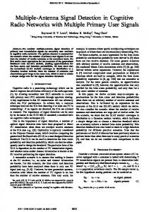
(14) Note that (14) has been previously derived in [5], while (13) is new. Condition p < n(m − n + 1): Observe that the condition p < n(m − n + 1), required for the moment expressions (13) and (14) to hold, is satisfied whenever p < n, with the value of n decreasing for increasing m − n. The first few moments can thus be obtained for even a very small number of antennas and observations. For example, for p = 3, the condition is satisfied when n = 2 and m = 3. Simulating H: To simulate the detection probability for the figures in this paper, we randomly choose H as ∼ CN n,k (0n,k , In ), which is then held constant for the m observation periods. This corresponds to a scenario where there is transmission from a single PU utilizing k antennas for spatial multiplexing, with unit average received power from each transmit antenna, and where the PU-SU channel undergoes Rayleigh fading. To motivate our c.d.f. expressions, we first define W0 − E [W0 ] Δ Z0 = . 2 E (W0 − E [W0 ])

m=5, 10, 20, 30, 50

−3

−4

−3

−2

−1

x

0

Fig. 1. Cumulative distribution function of Z0 =

1

2

W0 −E[W0 ] E[(W0 −E[W0 ])2 ]

with

n = 0.9m and k = n. The c.d.f. of a standard Gaussian is also shown for comparison. Convergence of the Z0 c.d.f. curve to the Gaussian curve as m increases is evident.

Moreover, the c.d.f. of W0 is approximated as η − E [W0 ] , μ , μ , μ FW0 (η) ≈ G √ W0 ,2 W0 ,3 W0 ,4 μW0 ,2

(19)

where μW0 ,p is the pth central moment of W0 , given by p p p− μW0 ,p = . (20) E W0 (−E [W0 ])

(15)

=0

Proof. Follows by applying the same procedure used to obtain [12, Eq. (196)], which involves finding the p.d.f. of a normalized random variable using a truncated Edgeworth expansion [11], and integrating to obtain the c.d.f. Accuracy: The function G(x, μ2 , μ3 , μ4 ) corresponds to a truncated Edgeworth expansion of an appropriately normalized random variable [11]. More terms can be added to G(x, μ2 , μ3 , μ4 ) with an expected increase in accuracy, however, for only a small number of terms in (16), high accuracy is already achieved. This can be observed in Figs. 2 and 3, which plot respectively the probability of false alarm PFA (η) vs. the detection threshold η, and the probability of detection PCD (η) vs. the detection threshold η. The ‘Analytical (Gaussian)’ curves correspond to a Gaussian approximation without any correction terms, i.e., replacing G(·) in (16) with G(x, . . .) = Φ(x), while the ‘Analytical (Correction)’ curves are plotted using (17) and (19). Finally, the ‘Analytical (Beta) [5]’ curves are plotted using the Beta function approximation introduced in [5]. For the false alarm probability curves in Fig. 2, we observe that the Gaussian approximation deviates from the ‘Monte Carlo’ simulated curves, except for n = 10, m = 20, justifying the use of additional correction terms. However, both ‘Analytical (Correction)’ and ‘Analytical (Beta) [5]’ curves closely match the ‘Monte Carlo’ simulated curves. For the detection probability curves in Fig. 3, we again observe deviation of the Gaussian approximation from the ‘Monte Carlo’ simulated curves. Moreover, we observe that

(17)

where μW1 ,p is the pth central moment of W1 , given by p

μW1 ,p = E [(W1 − E [W1 ]) ] p p p− = . E W1 (−E [W1 ])

−2

10

10

Fig. 1 plots the c.d.f. of Z0 for different number of observations m. For comparison, the c.d.f. of a standard Gaussian wth zero-mean and unit-variance is also shown. All curves are generated using Monte Carlo simulations. We observe that as m grows large, the c.d.f. curve for Z0 approaches the Gaussian curve. A similar observation is made for W1 (not shown due to space limitations). This motivates us to consider a Gaussian approximation for the c.d.f. of W0 and W1 , with additional correction terms obtained by the Edgeworth expansion [11]. It is convenient to first define the following function: x2

2 e− 2 Δ μ3 (x2 − 1) G(x, μ2 , μ3 , μ4 ) = Φ(x) − √ π 12( μ2 )3 (μ3 )2 4 μ4 − 3μ22 2 2 x(x − 3) + √ 3 x x − 10x + 15 + √ 4 μ2 12 μ2 (16) where x, μ2 , μ3 , μ4 ∈ R and Φ(x) = 12 1 + erf √x2 . Using this definition, we have the following: Proposition 1. The c.d.f. of W1 is approximated as η − E [W1 ] FW1 (η) ≈ G , μW1 ,2 , μW1 ,3 , μW1 ,4 √ μW1 ,2

−1

10

(18)

=0

3

4953


0

10

1

−1

m=15, n=4

10

m=10 n=4

0.9 0.8 Detection Probability, PD(η)

False Alarm Probability, PFA(η)

Monte Carlo Analytical (Gaussian) Analytical (Correction) Analytical (Beta) [5]

m=20, n=10

0.7 0.6 0.5

n = 2, 3, 4, 5, 6

0.4 0.3 0.2

−2

10

0.9

1

1.1

1.2

1.3

1.4

Detection Threshold, η

1.5

1.6

1.7

ROC curve Approximate Threshold

0.1 −3 10

1.8

10

−2

−1

0

10

10

False Alarm Probability, PFA(η)

Fig. 2. Probability of false alarm vs. detection threshold, with k = n.

Fig. 4. ROC curve (detection probability vs. false alarm probability) with n = 10n and k = n. The vertical dotted line at a false N0 = 6, m = 0.1 alarm probability of 0.01 is shown for convenience.

1 Monte Carlo Analytical (Gaussian) Analytical (Correction) Analytical (Beta) [5]

0.9

D

Detection Probability, P (η)

0.8

where μ ¯ = e(1 − c)

m=10 n=4

0.7 0.6 0.5

m=15, n=4

and

m=20, n=10

0.4

σ ¯ 2 = e2 (1 − c)

0.3

0.1

ln

1 1−c

−c

(23)

Proof. See Appendix B. 1

1.2

1.4

1.6

1.8

Detection Threshold, η

2

2.2

2.4

2.6

This suggests that the false alarm probability for large n and m can be approximated as n (η − μ ¯) 1 √ , (24) PFA (η) = 1 − FW0 (η) ≈ 1 − erf 2 2¯ σ2

Fig. 3. Probability of detection vs. detection threshold, with N0 = 5 and k = n.

except for n = 4, m = 15, the ‘Analytical (Beta) [5]’ curves are inaccurate for most detection probabilities. However, we observe that our ‘Analytical (Correction)’ curves closely match the ‘Monte Carlo’ simulated curves for all antenna/observation configurations.

and thus the minimum threshold which can satisfy a false alarm probability requirement of α0 can be approximated as √ 2¯ σ 2 −1 erf (1 − 2α0 ) . (25) η≈μ ¯+ n

IV. C. D . F. OF W0 : A SYMPTOTIC A NALYSIS

A natural question then is how large the number of antennas and observations have to be for this to be accurate. To investigate this, we plot in Figs. 4 and 5 for c = 0.1 and c = 0.2 respectively, the receive operating characteristics (ROC) curve, i.e., detection probability vs. false alarm probability. The ‘ROC curve’ is plotted using Monte Carlo simulations. The ‘Approximate Threshold’ circle corresponds to the ROC point with threshold calculated in (25) with a false alarm probability of α0 = 0.01. We observe that the approximate threshold (25) can achieve the false alarm probability of 0.01 for all n with relatively high accuracy, while also obtaining a high detection probability for sufficienty large m. As expected, we also observe in Figs. 4 and 5 that increasing c for the same n results in a lower detection probability, as less observations are utilized for detection.

Although the false alarm probability can be calculated for arbitrary number of antennas n and observations m using the moment expressions in (14), for sufficiently large n and m, it is more convenient to obtain an expression for the c.d.f. which can be more efficiently calculated. Moreover, we observed in Fig. 1 that for increasing n and m, the c.d.f. of a normalized W0 approached a Gaussian distribution. We now formalize this, and show in the following theorem the asymptotic convergence of W0 to a Gaussian distribution: Theorem 2. Let n → ∞ with

→ c ∈ (0, 1). Then4

d n (W0 − μ ¯) → N 0, σ ¯2

d 4x →

(22)

with e = 2.718281828....

0.2

0.8

2(1−c) c

1−c c

n m

(21)

y implies x converges in distribution to y.

4

4954


where Σ = HH† + In N0 Then by denoting D = {0 ≤ λn ≤ . . . ≤ λ1 < ∞}, we have5

1 0.9

E [W1p ] p n λ 1 i i=1 = p fΛ (λ1 , . . . , λn )dλ1 , . . . dλn n D n λ n1 i=1i n p eω i=1 λi a 1 d = p p fΛ (λ1 , . . . , λn )dλ1 , . . . dλn n dω p D n λ n ω=0 i=1 i n n(n−1) ym (−1) 2 b =1 = p n (yi − yj ) n =1 (m − )! ∞i