Multiple Sensor Detection of Process Phenomena in Laser Powder Bed Fusion Brandon Lane*, Eric Whitenton, Shawn Moylan National Institute of Standards and Technology, 100 Bureau Drive, Gaithersburg, MD, 20899, USA ABSTRACT Laser powder bed fusion (LPBF) is an additive manufacturing (AM) process in which a high power laser melts metal powder layers into complex, three-dimensional shapes. LPBF parts are known to exhibit relatively high residual stresses, anisotropic microstructure, and a variety of defects. To mitigate these issues, in-situ measurements of the melt-pool phenomena may illustrate relationships between part quality and process signatures. However, phenomena such as spatter, plume formation, laser modulation, and melt-pool oscillations may require data acquisition rates exceeding 10 kHz. This hinders use of relatively data-intensive, streaming imaging sensors in a real-time monitoring and feedback control system. Single-point sensors such as photodiodes provide the temporal bandwidth to capture process signatures, while providing little spatial information. This paper presents results from experiments conducted on a commercial LPBF machine which incorporated synchronized, in-situ acquisition of a thermal camera, high-speed visible camera, photodiode, and laser modulation signal during fabrication of a nickel alloy 625 AM part with an overhang geometry. Data from the thermal camera provides temperature information, the visible camera provides observation of spatter, and the photodiode signal provides high temporal bandwidth relative brightness stemming from the melt pool region. In addition, joint-time frequency analysis (JTFA) was performed on the photodiode signal. JTFA results indicate what digital filtering and signal processing are required to highlight particular signatures. Image fusion of the synchronized data obtained over multiple build layers allows visual comparison between the photodiode signal and relating phenomena observed in the imaging detectors. Keywords: laser powder bed fusion, additive manufacturing, thermography, photodetector
1. INTRODUCTION Laser powder bed fusion (LPBF) is an additive manufacturing technique which uses a high power, focused laser to melt thin layers of metal powder in specified geometries, which then can form geometrically complex and nearly fully dense metallic parts. Although use of LPBF is growing in industry, multiple challenges to broader adoption remain, including anisotropic and inhomogenous microstructure and material properties, defects including pores and voids, and large residual stresses and distortion. The laser process zone, including the melt pool and vicinity, entail very complex, dynamic, physical phenomena including high temperature gradients and heating/cooling rates 1,2. Although a LPBF part build may require dozens of hours to complete, the process is extremely fast at the scale of the laser process zone. For example, consider 20 μm powder particles and a laser scan rate of 2 m/s, which are within the range of commercial LPBF systems. In this scenario, the laser will melt 100 000 particles per second, which gives an order of magnitude estimate for the high potential sampling rates required for sensors to capture events at the melt pool scale. Many researchers and LPBF machine vendors have investigated monitoring of LPBF processes to develop and validate simulations and models, investigate methods for in-situ part qualification, develop sensing methods for feedback control, or simply advance understanding of underlying physical processes 3,4. Perhaps most notable is the use of non-contact photometric detectors that monitor melt pool transient signatures, and can provide radiant or thermal information. These include array detectors (imagers/cameras), which can provide spatial measurements, and single-point detectors such as *
[email protected]; phone: 1-301-975-5471 Official contribution of the National Institute of Standards and Technology (NIST); not subject to copyright in the United States. The full descriptions of the procedures used in this paper require the identification of certain commercial products. The inclusion of such information should in no way be construed as indicating that such products are endorsed by NIST or are recommended by NIST or that they are necessarily the best materials, instruments, software or suppliers for the purposes described.
Thermosense: Thermal Infrared Applications XXXVIII, edited by Joseph N. Zalameda, Paolo Bison, Proc. of SPIE Vol. 9861, 986104 · © 2016 SPIE · CCC code: 0277-786X/16/$18 · doi: 10.1117/12.2224390
Proc. of SPIE Vol. 9861 986104-1 Downloaded From: http://proceedings.spiedigitallibrary.org/ on 10/25/2016 Terms of Use: http://spiedigitallibrary.org/ss/termsofuse.aspx
pyrometers and photodetectors, which provide higher temporal bandwidth without spatial information. Melt pool monitoring (MPM) systems incorporating imagers and photodetectors are already appearing in commercial LPBF machines as a means for part quality assurance by observing relative changes in melt pool behavior throughout the volume of a part 3. However, spatial resolution is sacrificed in order to attain higher speed or frame rate. For example, Berumen et al. demonstrated 10 000 frame/s imaging of the melt pool, but was limited to using a 20 pixel x 16 pixel window 5. The streaming type of cameras used in that work, though limited in bandwidth by the data transmission interface (e.g., Cameralink or CoaXpress), can stream data continually to a processor such as a field-programmable gate array (FPGA), which can then compute melt-pool characteristic variables such as intensity, area, length, or width, and map to the XYZ coordinates of the LPBF part 6,7, or potentially be used as feedback control variables. Photodetectors or pyrometers provide much higher bandwidth, and have been used in conjunction with high speed imagers, aligned co-axially with the laser 5,8, or for viewing the process zone from the side 9. According to current literature, correlation of detector amplitude to process signatures is most often done in the time domain, where signal amplitude or standard deviation (as a measure of noise) is related to observed trends. Berumen et al. showed how photodetector amplitude and standard deviation of the signal increased with layer thickness, but also showed a decreasing trend attributed to contamination on the f-theta lens 5. Craeghs et al. noted that photodiode signal scaled with the melt pool area measured via a coaxially aligned imager 7. Doubenskaia et al. showed how pyrometer signal amplitude varied with different LPBF process parameters including powder layer thickness, hatch distance, and different laser scan strategies 8. Commercial companies, such as B6 Sigma Inc. (United States) or plasmo Industrietechnik GmbH (Austria), have incorporated photodetectors and/or pyrometers in their aftermarket monitoring and sensing systems for LPBF machines, however, the signal analysis algorithms and correlations to part or build quality are proprietary. Though they don’t give details on their algorithms, Grünberger et al. (from plasmo) indicate use of frequency analysis methods, and mention that an increase in higher frequency signal resulting from a ‘splashy’ melt pool can be attributed to unfavorable melt pool behavior and build quality 10. ‘Splashy’ behavior is also called sparking or spatter. Spatter is caused by high vapor flux on the surface of the melt pool, which causes a recoil pressure on the melt pool and pushes droplets of molten metal out of the pool 1. Though this leads to lower consolidation efficiency and is generally considered a deleterious phenomenon, there is little non-proprietary indepth research relating spatter characteristics to the build process or final part quality. The work described in this paper extends these previous investigations into combined use of high speed imaging and photodetectors, and focuses on the method for synchronization and data visualization, as well as provides preliminary observations which relate detector signals to observations from the high speed imagers. In addition, a joint-time frequency analysis (JTFA) method is applied to the photodetector signal, which details spectral content of the signal vs. time. The goal of this work is to provide physical basis for this spectral content of the photodetector signal by synchronous observation of the melt pool through the high speed visible and thermal cameras. This may provide basis for further sensor system design, and signal processing and filtering methods.
2. EXPERIMENT SETUP 2.1 High Speed Thermal and Visible Cameras and Data Acquisition A high speed data acquisition (DAQ) system was used to capture one analog channel (the photodetector), and six digital channels, which included triggering and video frame edges, as well as the laser modulation signal. Triggering was accomplished by using a handheld switch connected to industrial timers to create timed delays to the cameras. The DAQ system collected at 1 MHz over all channels. Thermal and visible video cameras were set up to capture on the cameras’ respective hard drives. The visible camera was set to capture 4000 frames/s. The DAQ system and camera computers are all monitored and operated via a ‘keyboard,video,mouse’ (KVM) switch. The thermal camera was positioned outside the build chamber and observed the build area through a custom door on the front of the machine and angled 43.7° onto the build plane, as shown in Figure 1, left. Details of the custom door and camera setup are given in 11. The high speed visible camera head was located within the build chamber in the upper right corner as viewed from the front of the machine, and data cables fed through a custom sealed through-port. Orientation and distance of the high speed visible camera were not measured. The thermal camera was operated at 1800 frames/s, 0.040 ms integration time, and corresponding to a thermal calibration range between 500 °C and 1025 °C over a dynamic range up to approximately 13000 digital levels (DLs), above which
Proc. of SPIE Vol. 9861 986104-2 Downloaded From: http://proceedings.spiedigitallibrary.org/ on 10/25/2016 Terms of Use: http://spiedigitallibrary.org/ss/termsofuse.aspx
the pixels start to saturate. The photodetector was aligned with and fastened to the top of the thermal camera’s 50 mm short-wave infrared (SWIR) lens, as shown in Figure 1, right. The detector housing was protected with plastic shrink tubing.
Build
Plane
Figure 1: Left: Relative orientation of externally mounted thermal camera and internally mounted high speed visible camera in the LPBF machine’s build chamber. Right: Image of photodetector fastened to the outside of the SWIR lens barrel.
2.2 Photodetector Circuit The photodiode is a typical silicon detector in a lensed metal case (TO-18) with relative spectral response between 300 nm and 1200 nm with peak at 850 nm. Figure 2 shows the detector circuit used. The diode, 470 μF electrolytic capacitor, and 0.1μF ceramic capacitor help provide a robust supply voltage. Frequency response of the detector was estimated by observing the step response from a light emitting diode (LED) source. Rise time of the detector was approximately 3 μs. Voltage output is attenuated by a factor of 0.707 at 141.5 kHz (cutoff frequency), with a slope of 0.1 per decade of frequency.
MRD500 SK3081 30 v Power Supply
470 μF 100v
0.1 μF
3.05 kΩ
Sensor Signal
Figure 2: Photodiode circuit.
It should be noted that no spectral filter was used in front of the photodetector, so the spectral responsivity does include laser wavelength (1070 nm). Large spikes in the detector signal are likely due to occasional stray laser light reflections. 2.3 LPBF Build Strategy A side-view schematic of the example LPBF part is shown in Figure 3, left, which investigates the effect of an overhanging structure. For this paper, data from only one build layer is explored, which occurred at a build height of 7.90 mm, although the overhanging structure continued to complete a 16 mm tall structure. The powder material is nickel alloy 625, which is used to build parts upon a custom alloy 625 substrate. The following build parameters were used to build the example part with a commercial LPBF system: Hatch distance: 0.1 mm, stripe width: 4 mm, stripe overlap: 0.1 mm, powder layer thickness: 20 µm, laser scan speed: 800 mm/s, laser power (during infill): 195 W. The pre-contour passes start at the lower left corner of the part (as viewed in Figure 3 right), and post-contour pass starts at the upper left. Both traverse in counter-clockwise around the part perimeter. The pre-contour pass uses a laser power of 100 W, post-contour uses 120 W, and both contours use 800 mm/s scan speed.
Proc. of SPIE Vol. 9861 986104-3 Downloaded From: http://proceedings.spiedigitallibrary.org/ on 10/25/2016 Terms of Use: http://spiedigitallibrary.org/ss/termsofuse.aspx
Thermal Camera + Photodetector View
40.5o Overhang
+z
Solid
7.90 mm Build Height
7.24 mm
Powder
Overhang Edge
1 st Stripe
+x
+y
+y 16 mm
16 mm
Figure 3:Left: Side-view schematic of overhang part at the layer observed in the example given in this paper (build height 7.90 mm). Right: Top-down geometric view of the build plane showing horizontal hatch pattern, stripe direction, and location of the overhang.
The scope of this paper focuses on the acquisition and initial processing of sensor data, therefore it only explores one example layer from the 16 mm tall part. Data was collected at 45 different build layers of the total 16 mm tall part. The analysis of the one layer described in this paper will form the basis for future analysis on all collected data, which will allow for interlayer comparisons.
3. SIGNAL PROCESSING AND ANALYSIS 3.1 Joint Time Frequency Analysis of Photodetector Signal Photodetectors provide high temporal bandwidth, but melt pool fluctuations and spatter can cause high-frequency stochastic fluctuations in the signal. Frequency spectrum analysis may provide better insight into changes in amplitude and frequency of these events. In addition, due to the semi-repetitive geometric nature of a LPBF scan strategy, it is important to acknowledge when certain events occur (e.g., when the laser changes direction or nears an area of interest such as a hole or overhang), so that the changes in signal spectrum may be interpreted in context. The time and frequency domains of the 1 MHz collected photodetector signal were processed using joint time frequency analysis (JTFA). JTFA is a suite of techniques for characterizing how the spectral content of a signal changes over time. In this paper, we use the Short-Time Fourier Transform (STFT) method with software developed by National Instruments in collaboration with the authors Qian and Chen 12. This method essentially computes a sequential Fourier Transform over data windows of specified length. The following parameters define the STFT method: ●
Length – How many data points are used in each Fourier Transform.
●
Freq Bins – Number of discrete sets of frequencies.
●
Window – Which function to convolve the data with to avoid aliasing. A Hanning function is used in this analysis.
●
Detrend – Parameter used to remove offset. A detrend of 0 is the original data, and detrend of 1 results in a flat line. As detrend goes from 0 to 1, the constant offset term and lower frequencies are removed more and more.
3.2 Merged Movies To better relate the JTFA and photodetector signal results to the thermal and visible camera images, a single video was created that consists of time-synchronized images from each detector or plot. These ‘merged movies’ are created using custom software written in Visual Basic that uses trigger and frame capture signals collected via the DAQ system, and chronologically synchronizes video and data streams into a single video. Figure 4 gives an example of one frame from the merged movie, and indicates the location of the different video and data feeds. A moving cursor was also included which indicates the current time location along the JTFA plots. Table 1 gives details of the parameters used to generate each JTFA plot. The photodetector signal is given as a scrolling plot of raw signal, as well as 750-point running average and standard deviation.
Proc. of SPIE Vol. 9861 986104-4 Downloaded From: http://proceedings.spiedigitallibrary.org/ on 10/25/2016 Terms of Use: http://spiedigitallibrary.org/ss/termsofuse.aspx
High Speed Visible
S0, S1, S2 A
Thermal Camera as-
B U
03
01- 04- 08 03- 03- 07 02- 06
-
C
Photodetector Signal
.- 01- 05 á
¢
00- 00- 04 Ql-
lÿW
D
Jl'
-03- 03-
.II
1'
d1-
Q3
q!.
412- ü2- 02 4.,
._L__it- .11_.a
Figure 4: Example frame of the merged movie detailing content of each sub-window. Movie frame playback is synchronized based on the high speed visible camera data. Specifications for each plot or video stream are listed in Table 1. Plots S0 through S2 appear at different times at the same location.
JTFA plots S0 to S2 in Figure 4 attempt to highlight particular time-periods of interest, and appear within the same location when those time periods occur in the camera and photodetector images. Plots S0 to S2 also use different processing parameters than plots A to D, and include a different time-synchronized data cursor. Table 1: Parameters used to generate each of the JTFA plots shown in the merged movie
JTFA Plot
Down Sample
Vertical Axis Limits
Detrend
Window Width
Notes
A
100:1
>0 Hz to 5 kHz
0.6
72.5 ms
Long window shows harmonics due to regular laser on/off cycling. Also shows other horizontal structure.
B
100:1
>0 Hz to 5 kHz
0.6
7.5 ms
Shorter window than A is slightly longer than one laser on/off cycle time.
C
10:1
>0 Hz to 50 kHz
0.6
7.25 ms
Similar window to B, but higher sample rate shows higher frequencies. Vertical stripes correspond to short duration events such as a bright flash or laser shutting off.
D
10:1
>0 Hz to 50 kHz
0.6
750 μs
Shorter window than C which yields more isolated islands of red.
S0
1:1
>0 Hz to 500 kHz
0.8
725 μs
Timespan: 0.422 s to 0.484 s, Highlights the first contour pass around the perimeter of the build layer.
S1
1:1
>0 Hz to 500 kHz
0.8
725 μs
Timespan: 0.550 s to 0.850 s, Highlights points just after laser passes near the overhang. Laser is scanning towards the photodetector, away from the overhang.
S2
1:1
>0 Hz to 500 kHz
0.8
725 μs
Timespan: 1.152 s to 1.452 s, highlights the center of a hatching scan when the melt pool is also within the field of view of the thermal camera.
Proc. of SPIE Vol. 9861 986104-5 Downloaded From: http://proceedings.spiedigitallibrary.org/ on 10/25/2016 Terms of Use: http://spiedigitallibrary.org/ss/termsofuse.aspx
4. SELECT RESULTS For the single layer example discussed here, a plethora of information is captured, all of which cannot be condensed into this paper. However, a few select observational examples are provided. True value in the data comes with comparison to post-processing analysis of the built part quality. Current efforts are underway to cut, polish, etch, and analyze the AM sample built in this example. 4.1 Time-resolved Phenomena The photodetector signal remained below 2 V the majority of the build layer, however large spikes exceeding 8 V were evident, and likely attributable to spurious reflections from the laser. Although spatter particles are very evident in the thermal and visible camera images, and single particularly bright particles may be traced in both, there is no obvious relationship between individual spatter particles and peaks in the photodetector signal. This may be expected, however, as the photodetector integrates the radiant emission from multiple occurring spatter particles, as well as the melt pool and plasma/metal vapor plume. In the thermal and visible video data, the amount and frequency of spatter, temperature gradients, and heating and cooling rates appeared largely consistent to previously published data which used the same material and scan parameters 11. However, as the melt pool approaches the overhang during the second and fourth stripes, and leaves the overhang at the beginning of the first and third stripe, the edge of the overhang incurs a much slower cooling rate compared to scan tracks in the center of the build area. Figure 5 gives examples of two frames from the thermal camera. After 37 ms, consisting of approximately seven back and forth hatching scans on the third stripe, the overhang remains at elevated temperature. Note that temperature values in Figure 5 are ‘apparent temperature’, which is the equivalent temperature if the surface were a perfect radiator ( = 1). Though not true temperature, apparent temperature can be assumed to be a minimum value, indicating the residual temperature at the overhang in Figure 5, right remains at least 700 °C more than 37 ms after formation. In addition, this residual heat at the overhang was also observable in the high speed visible camera, indicating the surface is still at visibly incandescent temperature. Apparent Temperature [°C] 20
1100
1 mm
Frame 2676 t = 1502.5 ms
20
Overhang Edge
40
40
60
60
80
80
100
1st Stripe 50
Frame 2744 1000 t = 1539.7 ms
3rd Stripe
800
800
600 120
100
150
200
250
300
350
1000 900
700
2nd Stripe
1100
900
100
120
1 mm
Residual heat at overhang
500 50
100
150
700
Melt pool continuing 3rd stripe 200
250
300
600
350
500
Figure 5: Two frames from the thermal camera apparent temperature data just after the overhang is exposed (left) and 68 frames after (right). The overhang is still at elevated temperature (within measureable range of the thermal camera) 37 ms after formation.
4.1.1 Comparison of Pre- and Post-Contour Exposure Pre- and post-contour exposures are of particular interest since they form the external, side surfaces of the part. As mentioned, the pre-contour pass started in the lower left corner of the build area and was 100 W laser power, while the post-contour started at the upper right and was 120 W. Both passes traversed counter-clockwise around the surface. Figure 6 shows the time-series photodetector signal during these periods. Overall, the signal was lower during the pre-contour compared to the post contour. In addition, the left and right edges had greater signal, which occurs when the melt pool was traveling towards or away from the photodetector, respectively. Observations in the camera feeds did not provide an obvious reason for this. The post-contour pass used 20% greater laser power, which should result in a larger melt pool. However, the thermal camera frames shown in Figure 7 show an additional rationale for why the post-contour photodetector signal was greater than the pre-contour. During the pre-contour pass, the melt pool is surrounded by a new powder layer, which is much less reflective than the new, solidified metal surface which the post-contour scans around. Reflections from the melt pool and spatter are very obvious on the solidified surface below the melt pool in Figure 7 right, and were very evident in the videos.
Proc. of SPIE Vol. 9861 986104-6 Downloaded From: http://proceedings.spiedigitallibrary.org/ on 10/25/2016 Terms of Use: http://spiedigitallibrary.org/ss/termsofuse.aspx
Photodetector Photodetector Signal Signal - [V] - [V]
2 2 1.5 1.5 1 1 0.5 0.5 0 0
Photodetector Photodetector Signal Signal - [V] - [V]
2 2 1.5 1.5 1 1 0.5 0.5 0 0
Pre-Contour Bottom Edge
430 430
Right Edge
440 440
Top Edge (Overhang)
450 450 Time - [ms] Time - [ms]
460 460
Left Edge
470 470
480 480
Post-Contour
Left Edge
Bottom Edge
2510 2510
2520 2520
Right Edge
2530 2530
Top Edge (Overhang)
2540 2540 Time - [ms] Time - [ms]
2550 2550
2560 2560
Figure 6: Comparison of photodetector signal during pre- and post-contour passes. Bottom, left, right, and top edge period labels refer to melt pool location with respect to Figure 3 right.
Pre-contour 20
1 mm
1. #+
40
20
....
40
1 mm700
700
600
600
500
500
400
400
60
60
80
80
300
100
100
200
120
Frame 812, t = 466.9 ms 50
100
150
120
200
Signal [DLs]
Post-contour
..
r
250
300
350
300
Residual heat from core exposure
Frame 812, t = 2561.9 ms 100 50
100
150
200
250
300
200 100
350
Figure 7: Example thermal video frames (raw camera signal) during pre- and post-contour scans along the top edge of the build layer. Higher reflectivity of the solid surface in the post-contour image shows greater reflection of spatter particles. In addition, residual heat from the last exposure on the fourth stripe is still evident along the top edge.
4.2 Frequency-resolved Phenomena JTFA plot C from Figure 4and Table 1 is selected as an example for analysis from plots A through D, and shown in Figure 8 with time periods indicated during each stripe. There was noticeably greater low and high frequency content during the first and third stripe when the laser is scanning toward the detector. During these scans, a less reflective powder exists between the melt pool and the detector, which would go against the hypothesis given in the previous section that reflections from spatter on the metallic surface are a prime reason for increased photodetector signal. However, the first and third stripe period also occur after the melt pool has left the overhang, which was shown to remain at elevated temperatures high enough to be observed in the visible spectrum high speed camera. A second hypothesis may be that while reflections contribute to the overall signal, changes in melt pool size may contribute more. Although the spatial resolution or magnification of both cameras is too low to observe transient changes in the melt pool size, it has been demonstrated experimentally 7 and in simulations 13 that melt pool size increases with underlying part temperature and/or proximity to overhangs, and melt pool size has been positively correlated to the signal of an observing single point detector 7 . This may also explain that the increase in detector signal occurs prior to the beginning of the third stripe when the melt pool is just approaching the overhang. Increased melt pool size and temperature likely correlate to more frequent or greater ejection of spatter particles, which would then contribute to more high frequency content in the photodetector signal in conjunction with the low frequency.
Proc. of SPIE Vol. 9861 986104-7 Downloaded From: http://proceedings.spiedigitallibrary.org/ on 10/25/2016 Terms of Use: http://spiedigitallibrary.org/ss/termsofuse.aspx
Second Stripe (Away from Camera)
First Stripe Pre-contour (Towards Camera)
Frequency - [kHz]
50
Third Stripe (Towards Camera)
Fourth Stripe (Away from Camera) Post-contour
40 30 20 10 0
500
1000
1500 Time - [ms]
2000
2500
Figure 8: JTFA plot C (10:1 downsampling, detrend 0.6, 7.25 ms window size).
5. CONCLUSIONS A synchronized thermal camera, high speed visible camera, and photodetector were used to measure an LPBF build consisting of an overhang structure. The photodetector signal was analyzed using joint-time frequency analysis, which provides a measure of frequency content of signal versus time. All video and signal feeds were synchronized and viewed in a single merged video to relate observations from each. Data from one layer at the approximate center of the 16 mm tall part is explored as an example in this paper. Residual heat and slower cooling rates were observed in the thermal and visible camera after the melt pool formed and then exited the overhang edge. These time periods also resulted in greater low and high frequency content of the photodetector signal. Two hypotheses were made regarding the photodetector signal: signal content is increased by the existence of spatter particle reflections on a solidified surface, and overall signal increases when the melt pool nears the overhang due to likely increases in melt pool size, temperature, and spatter frequency, and this effect is a greater contributor to overall signal levels. Overall, there was a strong relationship between photodetector signal and the location and motion of the melt pool with respect to the scan strategy. Filtering or processing of single point detector signals may require knowledge of the laser spot position (e.g., XYZ coordinates with respect to the part volume) in order to differentiate between periodic behavior stemming from the scan strategy, and to capture unique phenomena that might be indicative of a defect. In addition, there is likely a relationship between the location of the melt pool relative to the field of view of the photodetector. Future efforts will include measurement of a point illumination source signal to observe relative photodetector signal vs. location within the field of view. Since the frequency of events in this analysis potentially spans over five orders of magnitude of frequency, the Fourier transform based JTFA methods shown here required multiple processing parameter sets (e.g., downsampling, window size, frequency plot axis limits) to highlight low frequency content on the same scale as the higher. Further efforts will use least-squares spectral analysis (LSSA) using the Lomb-Scargle method 14. This method uses variable sample lengths that scale with frequency, which helps to display higher frequency signals on the same scale as the lower, whereas FT methods boost low frequency signal content.
REFERENCES [1]
[2] [3]
Khairallah, S. A., Anderson, A. T., Rubenchik, A.., King, W. E., “Laser powder-bed fusion additive manufacturing: Physics of complex melt flow and formation mechanisms of pores, spatter, and denudation zones,” Acta Mater. 108, 36–45 (2016). Kruth, J.-P., Levy, G., Klocke, F.., Childs, T. H. C., “Consolidation phenomena in laser and powder-bed based layered manufacturing,” CIRP Ann. - Manuf. Technol. 56(2), 730–759 (2007). Dunsky, C., “Process monitoring in laser additive manufacturing,” Ind. Laser Solut. 29(5) (2014).
Proc. of SPIE Vol. 9861 986104-8 Downloaded From: http://proceedings.spiedigitallibrary.org/ on 10/25/2016 Terms of Use: http://spiedigitallibrary.org/ss/termsofuse.aspx
[4]
[5] [6]
[7] [8] [9] [10] [11] [12] [13]
[14]
Mani, M., Lane, B., Donmez, M. A., Feng, S., Moylan, S.., Fesperman, R., “Measurement science needs for realtime control of additive manufacturing powder bed fusion processes,” NIST Interagency/Internal Report (NISTIR) 8036, National Institute of Standards and Technology, Gaithersburg, MD (2015). Berumen, S., Bechmann, F., Lindner, S., Kruth, J.-P.., Craeghs, T., “Quality control of laser- and powder bedbased Additive Manufacturing (AM) technologies,” Phys. Procedia 5, Part B, 617–622 (2010). Clijsters, S., Craeghs, T., Buls, S., Kempen, K.., Kruth, J.-P., “In situ quality control of the selective laser melting process using a high-speed, real-time melt pool monitoring system,” Int. J. Adv. Manuf. Technol. 75(5-8), 1089– 1101 (2014). Craeghs, T., Clijsters, S., Kruth, J.-P., Bechmann, F.., Ebert, M.-C., “Detection of process failures in Layerwise Laser Melting with optical process monitoring,” Phys. Procedia 39, 753–759 (2012). Doubenskaia, M., Pavlov, M., Grigoriev, S., Tikhonova, E.., Smurov, I., “Comprehensive optical monitoring of selective laser melting,” J. Laser Micro Nanoeng. 7(3), 236–243 (2012). Bayle, F.., Doubenskaia, M., “Selective laser melting process monitoring with high speed infra-red camera and pyrometer,” Proc SPIE 6985 Fundam. Laser Assist. Micro- Nanotechnologies 6985, 698505–698505 – 8 (2008). Grünberger, T.., Domröse, R., “Optical in‐process monitoring of direct metal laser sintering (DMLS),” Laser Tech. J. 11(2), 40–42 (2014). Lane, B., Moylan, S., Whitenton, E. P.., Ma, L., “Thermographic Measurements of the Commercial Laser Powder Bed Fusion Process at NIST,” Proc. Solid Free. Fabr. Symp., 575, Austin, TX (2015). Qian, S.., Chen, D., Joint Time-Frequency Analysis: Method and Application, Har/Dskt edition, Prentice Hall, Upper Saddle River, N.J (1996). King, W., Anderson, A. T., Ferencz, R. M., Hodge, N. E., Kamath, C.., Khairallah, S. A., “Overview of modelling and simulation of metal powder bed fusion process at Lawrence Livermore National Laboratory,” Mater. Sci. Technol. 31(8), 957–968 (2014). Scargle, J. D., “Studies in astronomical time series analysis. II-Statistical aspects of spectral analysis of unevenly spaced data,” Astrophys. J. 263, 835–853 (1982).
Proc. of SPIE Vol. 9861 986104-9 Downloaded From: http://proceedings.spiedigitallibrary.org/ on 10/25/2016 Terms of Use: http://spiedigitallibrary.org/ss/termsofuse.aspx