NANOTECHNOLOGY
MULTISCALE SIMULATION OF NANOSYSTEMS The authors describe simulation approaches that seamlessly combine continuum mechanics with atomistic simulations and quantum mechanics. They also discuss computational and visualization issues associated with these simulations on massively parallel computers.
E
ngineering mechanics provides excellent theoretical descriptions for the rational design of materials and accurate lifetime prediction of mechanical structures. This approach deals with continuous quantities such as strain field that are functions of both space and time. Constitutive relations such as Hooke’s law for deformation and Coulomb’s law for friction describe the relationships between these macroscopic fields. These constitutive equations contain material-specific parameters such as elastic moduli and friction coefficients,
1521-9615/01/$10.00 © 2001 IEEE
AIICHIRO NAKANO, MARTINA E. BACHLECHNER, RAJIV K. KALIA, ELEFTERIOS LIDORIKIS, PRIYA VASHISHTA, AND GEORGE Z. VOYIADJIS Louisiana State University
TIMOTHY J. CAMPBELL Logicon Inc. and Naval Oceanographic Office Major Shared Resource Center
SHUJI OGATA Yamaguchi University
FUYUKI SHIMOJO Hiroshima University
56
which are often size dependent. For example, the mechanical strength of materials is inversely proportional to the square root of the grain size, according to the Hall-Petch relationship. Such scaling laws are usually validated experimentally at length scales above a micron, but interest is growing in extending constitutive relations and scaling laws down to a few nanometers. This is because many experts believe that by reducing the structural scale (such as grain sizes) to the nanometer range, we can extend material properties such as strength and toughness beyond the current engineering-materials limit.1 In addition, widespread use of nanoelectromechanical systems (NEMS) is making their durability a critical issue, to which scaling down engineering-mechanics concepts is essential. Because of the large surface-to-volume ratios in these nanoscale systems, new engineeringmechanics concepts reflecting the enhanced role of interfacial processes might even be necessary. Atomistic simulations will likely play an important role in scaling down engineeringmechanics concepts to nanometer scales. Recent advances in computational methodologies and massively parallel computers have let researchers carry out 10- to 100-million-atom atomistic simulations (the typical linear dimen-
COMPUTING IN SCIENCE & ENGINEERING
Authorized licensed use limited to: UNIVERSITY OF OSLO. Downloaded on January 14, 2009 at 04:59 from IEEE Xplore. Restrictions apply.
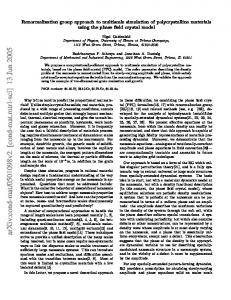
sion ranges from 50 to 100 nanometers) of real materials.2 To successfully design and fabricate novel nanoscale systems, we must bridge the gap in our understanding of mechanical properties and processes at length scales ranging from 100 nanometers (where atomistic simulations are currently possible) to a micron (where continuum mechanics is experimentally validated). To achieve this goal, scientists are combining continuum mechanics and atomistic simulations through integrated multidisciplinary efforts so that a single simulation couples diverse length scales. However, the complexity of these hybrid schemes poses an unprecedented challenge, and developments in scalable parallel algorithms as well as interactive and immersive visualization are crucial for their success. This article describes such multiscale simulation approaches and associated computational issues using our recent work as an example. The multiscale-simulation approach Processes such as crack propagation and fracture in real materials involve structures on many different length scales. They occur on a macroscopic scale but require atomic-level resolution in highly nonlinear regions. To study such multiscale materials processes, we need a multiscalesimulation approach that can describe physical and mechanical processes over several decades of length scales. Farid Abraham and his colleagues have developed a hybrid simulation approach that combines quantum-mechanical calculations with large-scale molecular-dynamics simulations embedded in a continuum, which they handle with the finite-element approach based on linear elasticity.3,4 Figure 1 illustrates such a multiscale FE– MD–QM simulation approach for a material with a crack. Let’s denote the total system to be simulated as S0. A subregion S1 (⊂ S0) near the crack exhibits significant nonlinearity, so we simulate it atomistically, whereas the FE approach accurately describes the rest of the system, S0 − S1. In the region S2 (⊂ S1) near the crack surfaces, bond breakage during fracture and chemical reactions due to environmental effects are important. To handle such chemical processes, we must perform QM calculations in S2, while we can simulate the subsystem, S1 − S2, with the classical MD method. Figure 1 also shows typical length scales covered by the FE, MD, and QM methods. In the following, we describe how an FE calculation can seamlessly embed an
Start Partition FE/MD/QM systems, S0 ⊃ S1 ⊃ S2
Compute FFE(S0–S1)
Compute FMD(S1–S2)
Compute FQM(S2)
102 to 10–7m
10–6 to 10–10m
10–9 to 10–11m
Update the systems No
Final step?
Yes
Stop
Figure 1. A hybrid finite-element, molecular-dynamics, quantummechanical simulation. The FE, MD, and QM approaches compute forces on particles (either FE nodes or atoms) in subsystems, S0 − S1 (represented by meshes), S1 − S2 (blue and red spheres), and S2 (yellow and green), respectively. The simulation then uses these forces in a time-stepping algorithm to update the positions and velocities of the particles. The figure also shows typical length scales covered by the FE, MD, and QM methods.
MD simulation, which in turn embeds a QM calculation. Hybrid FE–MD schemes
Continuum elasticity theory associates a displacement vector, u(r), with each point, r, in a deformed medium. The FE method tessellates space with a mesh. It discretizes the displacement field, u, on the mesh points (nodes) while interpolating the field’s values within the mesh cells (elements) from its nodal values. Equations of motion govern the time evolution of u(r); these equations are a set of coupled ordinary differential equations subjected to forces from surrounding nodes. This method derives the nodal forces from the potential energy, EFE[u(r)], which encodes how the system responds mechanically in the framework of elasticity theory. To study how atomistic processes determine macroscopic-materials properties, we can employ the MD method, in which we obtain the system’s phase-space trajectories (the positions and velocities
JULY/AUGUST 2001
Authorized licensed use limited to: UNIVERSITY OF OSLO. Downloaded on January 14, 2009 at 04:59 from IEEE Xplore. Restrictions apply.
57
HS
MD
FE
[1 1 1]
[1 1 1]
– [ 2 1 1]
– [0 1 1]
Figure 2. A hybrid FE–MD scheme for a silicon crystal. On the top is the MD region, where spheres represent atoms and lines represent atomic bonds. On the bottom is the FE region, where spheres represent FE nodes and FE cells are bounded by lines. The red box marks the handshake region, in which particles are hybrid nodes/atoms; the blue dotted line in the HS region marks the FE–MD interface. The left and right figures are views of the 3D crystalline system from two different crystallographic orientations, – – [011] and [211], respectively.
of all atoms at all times). Accurate atomic-force laws are essential for describing how atoms interact with each other in realistic simulations of materials. Mathematically, a force law is encoded in the interatomic potential energy, EMD(rN), which is a function of the positions of all N atoms, rN = {r1, r2, ..., rN}, in the system. In the past years, we have developed reliable interatomic-potential models for a number of materials, including ceramics and semiconductors.5 Our many-body interatomic potential scheme expresses EMD(rN) as an analytic function that depends on relative positions of atomic pairs and triples. The pair terms represent steric repulsion between atoms, electrostatic interaction due to charge transfer, and induced charge–dipole and dipole–dipole interactions that take into account the large electronic polar-
58
izability of negative ions. The triple terms take into account covalent effects through the bending and stretching of atomic bonds. We validate the interatomic potentials by comparing various calculated quantities with experiments. These include lattice constants, cohesive energy, elastic constants, melting temperatures, phonon dispersion, structural transformation pressures, and amorphous structures. A set of coupled ordinary differential equations, similar to those for FE nodes, govern the time evolution of rN. Hybrid FE–MD schemes spatially divide the physical system into FE, MD, and handshake regions.3,4 In the FE region, these schemes solve equations for continuum elastic dynamics on an FE mesh. To make a seamless transition from the FE to MD regions, these schemes refine the FE mesh in the HS region down to the atomic scale near the FE–MD interface such that each FE node coincides with an MD atom.3,4 The FE and MD regions are made to overlap over the HS region, establishing a one-to-one correspondence between the atoms and the nodes. Figure 2 illustrates an FE–MD scheme. On the top is the atomistic region (crystalline silicon in this example), and on the bottom is the FE region. The red box marks the HS region, in which particles are hybrid nodes/atoms, and the blue dotted line in the HS region marks the FE–MD interface. These hybrid nodes/atoms follow hybrid dynamics to ensure a smooth transition between the FE and MD regions. The scheme by Abraham and his colleagues defines an explicit energy function, or Hamiltonian, for the transition zone to ensure energyconserving dynamics.3,4 All finite elements that cross the interface contribute one-half of their weight to the potential energy. Similarly, any MD interaction between atomic pairs and triples that cross the FE–MD interface contributes onehalf of its value to the potential energy. We use a lumped-mass scheme in the FE region; that is, we assign the mass on nodes instead of distributing it continuously within an element.3,4 This reduces to the correct description in the atomic limit, where nodes coincide with atoms. To rapidly develop an FE–MD code by reusing an existing MD code, we exploited formal similarities between the FE and MD dynamics. In our FE–MD program, particles are either FE nodes or MD atoms, and a single array stores their positions and velocities. The FE method requires additional bookkeeping, because each element must be associated with its corresponding nodes. Our program efficiently performs this by
COMPUTING IN SCIENCE & ENGINEERING
Authorized licensed use limited to: UNIVERSITY OF OSLO. Downloaded on January 14, 2009 at 04:59 from IEEE Xplore. Restrictions apply.
using the linked cell list in the MD code. Parallel computing requires decomposing the computation into subtasks and mapping them onto multiple processors. For FE–MD simulations, a divide-and-conquer strategy based on spatial decomposition is possible.6,7 (Task decomposition has previously been used between FE and MD tasks.3,4) This strategy divides the system’s total volume into P subsystems of equal volume and assigns each subsystem to a processor in an array of P processors. It then assigns the data associated with a subsystem’s particles (either FE nodes or MD atoms) to the corresponding processor. For this strategy to calculate the force on a particle in a subsystem, the coordinates of the particles in the boundaries of neighbor subsystems must be “cached” from the corresponding processors. After an updating of the particle positions due to a time-stepping procedure, some particles might have moved out of the subsystem. These particles “migrate” to the proper neighbor processors. With the spatial decomposition, the computation scales as N/P while communication scales in proportion to (N/P)2/3 for an N-particle system. The communication overhead thus becomes less significant when N (typically 106 to 109) is much larger than P (102 to 103)—that is, for coarse-grained applications. The unified treatment of atoms and nodes with regular spatial decomposition could cause load imbalance among processors. However, load-balancing schemes developed for MD simulations can easily solve this problem.6,7 To validate our FE–MD scheme, we simulated a projectile impact on a 3D block of crystalline silicon (see Figure 3). The block has dimensions of– 10.5 nanometers and 6.1 nanometers along the – [211] and [011] and crystallographic orientations, respectively, and we impose periodic boundary conditions in these directions. Along the [111] direction, the system consists of a 11.5-nanometer-thick MD region, a 0.63-nanometer-thick HS region, and a 19.6-nanometer-thick FE region. The top surface in the MD region is free, and the nodes at the bottom surface in the FE region are fixed. The fully 3D FE scheme uses 20-node brick elements for the region far from the HS region, which provide a quadratic approximation for the displacement field and are adequate for continuum. In the scaled-down region close to the FE–MD interface, we switch to eight-node brick elements, which provide a linear approximation for the displacement field. In the HS region, we distort the elements to exhibit the same
[1 1 1]
1.8 ps
3.8 ps
– [ 2 1 1]
4.8 ps ∆r (Å) .50
FE HS MD
.25
.00
Figure 3. Time evolution of FE nodes and MD atoms in a hybrid FE–MD simulation of a projectile impact on a silicon crystal. Absolute displacement of each particle from its equilibrium position is color-coded. The figure shows a thin slice of the crystal for clarity of presentation.
lattice structure as crystalline silicon. In addition to these elements, we use prism-like elements for coarsening the FE mesh from the atomic to larger scales. We approximate the projectile with an infinite-mass hard sphere with a 1.7-nanometer radius, from which the silicon atoms scatter elastically. A harmonic motion of the projectile along the [111] direction creates smallamplitude waves in the silicon crystal. Figure 3 presents snapshots at three different times, showing only a thin slice for clarity of presentation. The color denotes the absolute displacement from the equilibrium positions measured in Å. The induced waves in the MD region propagate into the FE region without reflection, demonstrating seamless handshaking between MD and FE. In the hybrid FE–MD schemes we just described, a small number of elastic constants represent linear elastic properties of materials. Such a macroscopic approach does not necessarily connect with atomistics seamlessly when the size of finite elements is comparable to atomic spacing. For example, the FE analysis assumes that the energy density spreads smoothly throughout each element, but at the atomic scale, discreteness of atoms comes into play. Recent, more accurate methods construct constitutive relations from underlying atomistic calculations; they recover the correct atomic forces when the mesh is collapsed to the atomic spacing. The quasicontinuum method of Ellad Tadmor, Michael Ortiz, and Rob Phillips derives each element’s potential energy from microscopic
JULY/AUGUST 2001
Authorized licensed use limited to: UNIVERSITY OF OSLO. Downloaded on January 14, 2009 at 04:59 from IEEE Xplore. Restrictions apply.
59
interatomic potentials.8 This method assigns a representative crystallite in each element. It then deforms the crystallite according to the local deformation inside the element and assigns the crystallite’s total energy to the element. Robert Rudd and Jeremy Broughton’s coarse-grained MD method derives constitutive relations for continuum directly from the interatomic potential by means of a statistical coarse graining procedure.4 For the actual atomic configuration within the elements, their method calculates the dynamical matrix and transforms it to an equivalent dynamical matrix for the nodes. For atomic-size elements, the atomic and nodal degrees of freedom are equal in number and they obtain the MD dynamics. For large elements, they recover the continuum elasticity equations of motion. This method constitutes a perfectly seamless coupling of length scales but has high computational complexity. Hybrid MD–QM schemes
Empirical interatomic potentials used in MD simulations fail to describe chemical processes. Instead, to calculate interatomic interaction in reactive regions, we need a QM method that can describe bond breakage and formation. Interest has grown in developing hybrid MD–QM simulation schemes in which a reactive region treated by a QM method is embedded in a classical system of atoms interacting through an empirical interatomic potential. An atom consists of a nucleus and surrounding electrons, and QM methods treat electronic degrees of freedom explicitly, thereby describing the wave-mechanical nature of electrons. One of the simplest QM methods is based on tight binding.3,4 TB does not involve electronic wave functions explicitly but solves an eigenvalue problem for the matrix that represents interference between electronic orbitals. The spectrum of the eigenvalues gives the information on electronic density of states. TB derives the electronic contribution to interatomic forces through the Helmann-Feynman theorem, which states that only partial derivatives of the matrix elements with respect to rN contribute to forces. A more accurate but compute-intensive QM method deals explicitly with electronic wave functions,
{
}
Ψ N wf (r ) = Ψ1(r ), Ψ2 (r ), K , ΨN wf (r )
(Nwf is the number of independent wave functions, or electronic bands, in the QM calcula-
60
tion), and their mutual interaction in the framework of the density functional theory9,10 and electron–ion interaction using pseudopotentials.11 The DFT (for the development of which Walter Kohn received a 1998 Nobel chemistry prize) reduces the exponentially complex quantum many-body problem to a self-consistent eigen3 value problem that can be solved with O(N wf ) operations. With DFT, we can not only obtain accurate interatomic forces from the HelmannFeynman theorem, but also calculate electronic information such as charge distribution. The quantum-chemistry community has extensively developed hybrid MD–QM schemes.12 Various hybrid schemes combining both a molecular orbital method with varying degrees of quantum accuracy and a classical molecular mechanics method simulate chemical and biological processes in solution. The hybrid MO–MM schemes usually terminate a dangling-bond artifact at the MO–MM boundary by introducing a hydrogen (H) atom in the MO calculation. The hybrid simulation approach of Abraham and his colleagues uses a semiempirical TB method as a QM method and introduces an HS Hamiltonian to link the MD–TB boundary.3,4 Markus Eichinger and his colleagues have developed a hybrid MD–QM scheme based on the DFT for simulating biological molecules in a complex solvent.13 This scheme uses plane waves11 as the basis to solve the Kohn-Sham equations9 in the DFT. Such a plane-wave-based scheme, however, is difficult to implement for thousands of atoms on massively parallel computers, because it uses the fast Fourier transform, which involves considerable communication overhead. Recent efficient parallel implementations of DFT calculations represent wave functions and pseudopotentials on uniform real-space mesh points in Cartesian coordinates.14,15 These implementations perform the calculations in real space using orthogonal basis functions and a high-order finite difference method. The multigrid method can further accelerate real-space DFT calculations.15 Spatial-decompositionbased parallel implementation of the real-space methods is straightforward; systems containing a few thousand atoms can be simulated quantummechanically on 100 to 1,000 processors. We have developed a hybrid scheme for dynamic simulations of materials on parallel computers that embeds a QM region in an atomistic region.16 A real-space multigrid-based DFT14,15 describes the motion of atoms in the QM region,
COMPUTING IN SCIENCE & ENGINEERING
Authorized licensed use limited to: UNIVERSITY OF OSLO. Downloaded on January 14, 2009 at 04:59 from IEEE Xplore. Restrictions apply.
and the MD method describes it in the surrounding region. To partition the total system into the cluster and its environmental regions, we use a modular approach based on a linear combination of QM and MD potential energies. This approach consequently requires minimal modification of existing QM and MD codes:12 system
E = E CL
system
MD–FE Initial atomic positions and velocities
system Calculate classical forces(FCL, ) i in the system
cluster cluster + EQM − E CL
where ECL is the classical semiempirical potential energy for the whole system and the last two terms encompass the QM correction to that cluster energy. EQM is the QM energy for an atomic cluster cut out of the total system (its dangling bonds are terminated by hydrogen atoms— cluster handshake H’s). ECL is the semiempirical potential energy of a classical cluster that replaces handshake H’s with appropriate atoms. This approach requires calculating both QM and MD potential energies for the cluster. It introduces termination atoms in both calculations for the cluster. A unique scaled-position method treats HS atoms linking the cluster and the environment. This method determines the positions of HS atoms as functions of the original atomic positions in the system. Different scaling parameters in the QM and classical clusters relate the HS atoms to the termination atoms. We implement our hybrid scheme on massively parallel computers by first dividing processors into the QM and the MD calculations (task decomposition) and then using spatial decomposition in each task. The parallel program is based on message passing and follows the Message Passing Interface standard.17 We first place processors into MD and QM groups by defining two MPI communicators. (A communicator is an MPI data structure that represents a dynamic group of processes with a unique ID called context.) We write the code in the single-program, multiple-data (SPMD) programming style, so that each processor executes an identical program. We use selection statements for the QM and the MD processors to execute only the QM and the MD code segments, respectively. To reduce the memory size, we use dynamic memory allocation and deallocation operations in Fortran 90 for all the array variables. Figure 4 shows a flowchart of the parallel computations. First, spatial decomposition decomposes the total system into subdomains, each of which is mapped onto an MD processor. The MD processors calculate the classical potential system energy, ECL , and corresponding atomic forces,
QM nodes
Cluster data cluster Calculate classical forces(FCL, ) i in the cluster
cluster
(FQM,i )
Calculate quantum-mechanical cluster ) forces (FQM, i in the cluster
Calculate total forces in the system: cluster cluster (Fi = FCL,system + FQM, i i – FCL,i )
Update atomic positions and velocities
No Last step?
Figure 4. A flowchart of the parallel computations in our hybrid FE–MD–QM simulation algorithm.
using an empirical interatomic potential. Second, atomic data for the cluster and the HS atoms that are necessary to create the H-terminated cluster are transferred to the QM processors. Third, the QM processors perform DFT cluster calculations to obtain EQM and atomic forces for the H-terminated cluster, while the MD cluster processors calculate ECL and atomic forces for the classically terminated cluster, using the empirical interatomic potential. The real-space multigrid-based DFT code is parallelized by decomposing the mesh points to subdomains and then distributing them into the QM processors. The MD processors collect the energy and forces from QM and MD calculations. Finally, the MD processors calculate the total potential energy, E, and atomic forces, which in turn are used for time integration of the motion equations to update atomic positions and velocities. We applied the hybrid MD–QM simulation code to oxidation of a silicon surface. Figure 5 shows snapshots of the atomic configuration at 50 and 250 femtoseconds; atomic kinetic energies are color-coded. We see that dissociation energy released at the reaction of an oxygen
JULY/AUGUST 2001
Authorized licensed use limited to: UNIVERSITY OF OSLO. Downloaded on January 14, 2009 at 04:59 from IEEE Xplore. Restrictions apply.
61
(a)
(b)
(c)
Figure 5. A hybrid MD–QM simulation of oxidation of a silicon (100) surface. In the (a) initial configuration, magenta spheres are the cluster silicon atoms, gray spheres are the environment silicon atoms, yellow spheres are termination hydrogen atoms for QM calculations, blue spheres are termination silicon atoms for MD calculations, and green spheres are cluster oxygen atoms. In the snapshots at (b) 50 and (c) 250 femtoseconds, colors represent the kinetic energies of atoms in Kelvin.
molecule with silicon atoms in the cluster region transfers seamlessly to silicon atoms in the environment region. Owing to the formal similarity between parallel MD and FE–MD codes and the modularity of the MD–QM scheme, embedding a QM subroutine in a parallel FE–MD code to develop a parallel FE–MD–QM program is straightforward, as Figure 4 shows. Scalable FE–MD–QM algorithms
The FE scheme calculates the force elementby-element. And, with the lumped-mass approximation, it performs temporal propagation nodeby-node with O(Nnode) operations in a highly scalable manner (Nnode is the number of FE nodes). Atomistic study of process zones including mesoscale processes (dislocations and grains) requires that the MD region covers length scales
62
on the order of a micron ( N ~ 109 atoms); such large-scale MD simulations require highly scalable algorithms. Currently, the most serious bottleneck for large-scale FE–MD–QM simulations is the computational complexity of QM calculations. To investigate collective chemical reactions at oxidation fronts or at frictional interfaces, the QM region must cover length scales of 1 to 10 nanometers (approximately 103 to 104 atoms). Embedding a 104-atom QM calculation in 109atom MD is only possible with scalable algorithms for both MD and QM simulations. We have developed a suite of scalable MD and QM algorithms for materials simulations.18 Our scalable parallel MD algorithms employ multiresolutions in both space and time.6 We formulate the DFT calculation as a minimization of the energy, EQM(rN, ψNwf) with respect to ψ Nwf, with orthonormalization constraints among the electron wave functions, which is conventionally 3 solved by O(N wf ) operations. Researchers have proposed several O(Nwf) DFT methods based on a real-space grid.19 These methods constrain each one-electron wave function in a local region and avoid orthogonalization of wave functions. We use the energyfunctional minimization approach, which requires neither explicit orthogonalization nor inversion of an overlap matrix but instead involves unconstrained minimization of a modified energy function. Because the wave functions are localized in this approach, each wave function interacts with only those in the overlapping local regions. In each MD step, the conjugate-gradient (CG) method iteratively minimizes the energy function. Because the energy-minimization loop contains neither a subspace diagonalization nor the Gram-Schmidt orthonormalization, the computation time scales as O(Nwf/P) on P processors. The communication data size between neighboring nodes to calculate the kinetic-energy operator scales as O((Nwf/P)2/3) in the linearscaling DFT algorithm, which is in contrast to the O(Nwf(Nwf/P)2/3) communication in the conventional DFT algorithm. Global communication for calculating overlap integrals of the wave 2 functions, which scales as Nwf logP in the conventional DFT algorithm, is unnecessary in the linear-scaling algorithm. Figure 6 shows the computation time as a function of the number of simulated atoms for our linear-scaling MD and DFT algorithms on 1,024 IBM SP3 processors at the Naval Oceanographic Office Major Shared Resource Center. (For the DFT algorithm, we assume that each
COMPUTING IN SCIENCE & ENGINEERING
Authorized licensed use limited to: UNIVERSITY OF OSLO. Downloaded on January 14, 2009 at 04:59 from IEEE Xplore. Restrictions apply.
Immersive and interactive visualization The large-scale multiscale simulations we’ve discussed will generate enormous quantities of data. For example, a billion-atom MD simulation produces 100 Gbytes of data per frame including atomic species, positions, velocities, and stresses. Interactive exploration of such large datasets is important for identifying and tracking atomic features that cause macroscopic phenomena. Immersive and interactive virtual environments are an ideal platform for such explorative visualization. We are designing algorithms to visualize large-scale atomistic simulations in 3D immersive and interactive virtual environments. Our approach employs adaptive and hierarchical data structures for efficient visibility culling and levels-of-detail control for fast rendering. To achieve interactive-walkthrough speed and low access times in billion-atom systems, we employ an octree data structure and extract the regions of interest at runtime, thereby minimizing the size of the data sent to the rendering system (see Figure 7).22 We obtain the octree data structure by recursively dividing the physical system into smaller cells. We use standard visibilityculling algorithms to extract only the atoms that
Wall clock time (seconds per MD step)
MD step requires three self-consistent iterations of the Kohn-Sham equations9 with 40 CG iterations per self-consistent iteration. To simulate gallium arsenide systems, the DFT calculations include two independent electron wave functions per atom.) The figure shows that the computation involved in both the MD and DFT algorithms scales linearly with the number of atoms. The largest simulations include an 6.44billion-atom silica system for MD and a 111,000-atom gallium arsenide system for QM. Communication time in these calculations is negligible compared with computation time. Figure 6 also shows computation time for a variable-charge MD algorithm.20,21 This semiempirical approach allows the study of certain chemical reactions such as oxidation with much less computational complexity than with the DFT. This approach determines atomic charges at every MD step to equalize electronegativities of all the atoms. Considering the long computation time of the DFT algorithm compared with MD in Figure 6, such computationally less demanding semiempirical approaches to incorporating chemical reactions in multiscale simulations continue to be important.
Figure 6. The computation time of MD and QM algorithms on 1,024 IBM SP3 processors. The figure shows wall clock time as a function of the number of atoms for three linear-scaling schemes: classical MD of silica based on manybody interatomic potentials (circles); environment-dependant, variable-charge MD of alumina (squares); and a self-consistent QM scheme based on the DFT (triangles). Lines show ideal linear-scaling behaviors.
fit in the viewer’s field of view. The rendering algorithm uses a configurable multiresolution scheme to improve the walkthrough experience’s performance and visual appeal. This scheme individually draws each atomic entity at resolutions ranging from a point to a sphere, using from eight to 1,000 polygons for each entity. An OpenGL display list (a fast and convenient way to organize a set of OpenGL commands) for each type of atom is generated at all possible resolutions, because it is more efficient than individual function calls. At runtime, a particular resolution is called for each atom on the basis of the distance between the viewer and object. To accelerate the rendering and scene update, we use textures. We employ • billboarding for displaying the atoms and • large texture maps to increase the depth. Theoretically, these techniques will decrease the number of polygons to be displayed. However, accounting for the user perspective requires additional calculations. This can involve situations where slight changes in the user view make certain objects visible.
JULY/AUGUST 2001
Authorized licensed use limited to: UNIVERSITY OF OSLO. Downloaded on January 14, 2009 at 04:59 from IEEE Xplore. Restrictions apply.
63
Figure 7. An octree data structure for culling. Octree cells (bounded by white lines) dynamically approximate the current visible region (the arrow represents the viewer’s position and viewing direction). Only the visible atoms are processed for rendering.
We have implemented this system in an ImmersaDesk virtual environment (see Figure 8). The ImmersaDesk consists of a pivotal screen, an Electrohome Marquee stereoscopic projector, a head-tracking system, an eyewear kit, infrared emitters, a wand with a tracking sensor, and a wand-tracking I/O subsystem. A programmable wand with three buttons and a joystick allows interactions between the viewer and simulated objects. The rendering system is an SGI Onyx with two R10000 processors, 4 Gbytes of system RAM, and an InfinityReality2 graphics pipeline; it can render walkthroughs of multimillion-atom systems. However, it cannot handle multibillion-atom systems. For visualization at such large scales, we are exploring parallel processing on a cluster of PCs for data management and dedicating the SGI system to rendering. A scheme that predicts the user’s next movement and prefetches data from the cluster would also be advantageous.
64
M
odern MD simulations of materials started in 1964 when Aneesur Rahman simulated 864 argon atoms on a CDC 3600 computer.23 Assuming a simple exponential growth, the number of atoms that classical MD simulations can handle has doubled every 19 months to reach 6.44 billion atoms. Similarly, the number of atoms in DF–MD simulations (started by Roberto Car and Michelle Parrinello in 1985 for eight silicon atoms) has doubled every 12 months to 111,000. In the next 10 years, petaflop computers will maintain the growth rates in these “MD Moore’s laws,” and we will be able to perform 1012-atom classical and 107-atom quantum MD simulations. Multiresolution approaches, combined with cache-conscious techniques, will be essential to achieve scalability on petaflop architectures. Ingenious use of multiscale FE–MD–QM simulations implemented with such scalable al-
COMPUTING IN SCIENCE & ENGINEERING
Authorized licensed use limited to: UNIVERSITY OF OSLO. Downloaded on January 14, 2009 at 04:59 from IEEE Xplore. Restrictions apply.
gorithms will play a significant role in nanoscale materials research. However, many problems remain. For example, ill-conditioned minimization prohibits the practical application of current linear-scaling DFT algorithms.19 This is due to the localization approximation that destroys the invariance of the energy under unitary transformations of the wave functions. Designing a scalable library of well-conditioned, fast FE–MD–QM algorithms that work for a wide range of applications will be one of the most exciting challenges in computational science and engineering in the next 10 years.
Acknowledgments We carried out parts of the research presented in this article in collaboration with Xinlian Liu, Paul Miller, and Ashish Sharma at Louisiana State University and DeAndra Hayes at Xavier University. We thank Leslie F. Greengard, S. Lennart Johnsson, Efthimios Kaxiras, Pramod P. Khargonekar, Wolfgang G. Knauss, Peter A. Kollman, Anupam Madhukar, Krishnaswamy Ravi-Chandar, Viktor K. Prasanna, James R. Rice, and Robert O. Ritchie for stimulating discussions. This work is partially supported by the Air Force Office of Scientific Research, the Department of Energy, NASA, the National Science Foundation, and the USC-LSU Multidisciplinary Research Program of the University Research Initiative. We performed some million-atom simulations using in-house parallel computers at LSU’s Concurrent Computing Laboratory for Materials Simulations. We performed 10-million- to billion-atom simulations using parallel computers at the Department of Defense’s Major Shared Resource Centers under a DoD Challenge project.
Figure 8. A scientist immersed in an atomistic model of a fractured ceramic nanocomposite. This system is a silicon nitride ceramic matrix reinforced with silica-coated silicon carbide fibers. Small spheres represent silicon atoms; large spheres represent nitrogen (green), carbon (magenta), and oxygen (cyan) atoms.
5. P. Vashishta et al., “Molecular Dynamics Methods and LargeScale Simulations of Amorphous Materials,” Amorphous Insulators and Semiconductors, M.F. Thorpe and M.I. Mitkova, eds., Kluwer Academic Publishers, Dordrecht, Netherlands, 1996, pp. 151–213. 6. A. Nakano, R.K. Kalia, and P. Vashishta, “Scalable MolecularDynamics, Visualization, and Data-Management Algorithms for Materials Simulations,” Computing in Science & Eng., vol. 1, no. 5, Sept./Oct. 1999, pp. 39–47. 7. A. Nakano, “Multiresolution Load Balancing in Curved Space: The Wavelet Representation,” Concurrency: Practice and Experience, vol. 11, 1999, pp. 343–353. 8. E.B. Tadmor, M. Ortiz, and R. Phillips, “Quasicontinuum Analysis of Defects in Solids,” Philosophical Magazine A, vol. 73, 1996, pp. 1529–1563. 9. P. Hohenberg and W. Kohn, “Inhomogeneous Electron Gas,” Physical Rev., vol. 136, 1964, pp. B864–B871. 10. R. Car and M. Parrinello, “Unified Approach for Molecular Dynamics and Density Functional Theory,” Physical Rev. Letters, vol. 55, 1985, pp. 2471–2474.
References 1. M.C. Roco, S. Williams, and P. Alivisatos, eds., Nanotechnology Research Directions: IWGN Workshop Report, World Technology Division, Int’l Technology Research Inst., Loyola College, Baltimore, 1999, http://itri.loyola.edu/nano/IWGN.Research. Directions (current 21 May 2001). 2. A. Pechenik, R.K. Kalia, and P. Vashishta, Computer-Aided Design of High-Temperature Materials, Oxford Univ. Press, Oxford, UK, 1999.
11. M.C. Payne et al., “Iterative Minimization Techniques for Ab Initio Total Energy Calculations: Molecular Dynamics and Conjugate Gradients,” Rev. Modern Physics, vol. 64, 1992, pp. 1045–1097. 12. S. Dapprich et al., “A New ONIOM Implementation in Gaussian 98: I. The Calculation of Energies, Gradients, Vibrational Frequencies, and Electric Field Derivatives,” J. Molecular Structure: Theochem, vols. 461–462, 1999, pp. 1–21.
3. F.F. Abraham et al., “Spanning the Length Scales in Dynamic Simulation,” Computers in Physics, vol. 12, 1998, pp. 538–546.
13. M. Eichinger et al., “A Hybrid Method for Solutes in Complex Solvents: Density Functional Theory Combined with Empirical Force Fields,” J. Chemical Physics, vol. 110, 1999, pp. 10452–10467.
4. R.E. Rudd and J.Q. Broughton, “Concurrent Coupling of Length Scales in Solid State Systems,” Physica Status Solidi B, vol. 217, 2000, pp. 251–291.
14. J.R. Chelikowsky et al., “Electronic Structure Methods for Predicting the Properties of Materials: Grids in Space,” Physica Status Solidi B, vol. 217, 2000, pp. 173–195.
JULY/AUGUST 2001
Authorized licensed use limited to: UNIVERSITY OF OSLO. Downloaded on January 14, 2009 at 04:59 from IEEE Xplore. Restrictions apply.
65
15. J. Bernholc, “Computational Materials Science: The Era of Applied Quantum Mechanics,” Physics Today, vol. 52, no. 9, 1999, pp. 30–35. 16. S. Ogata et al., “Hybrid Finite-Element/Molecular-Dynamics/Electronic-Density-Functional Approach to Materials Simulations on Parallel Computers,” to be published in Computer Physics Comm. 17. W. Gropp, E. Lusk, and A. Skjellum, Using MPI, 2nd ed., MIT Press, Cambridge, Mass., 1994. 18. F. Shimojo et al., “A Scalable Molecular-Dynamics-Algorithm Suite for Materials Simulations: Design-Space Diagram on 1,024 Cray T3E Processors,” Future Generation Computer Systems, vol. 17, 2000, pp. 279–291. 19. S. Goedecker, “Linear Scaling Electronic Structure Methods,” Rev. Modern Physics, vol. 71, 1999, pp. 1085–1123. 20. F.H. Streitz and J.W. Mintmire, “Electrostatic Potentials for MetalOxide Surfaces and Interfaces,” Physical Rev. B, vol. 50, 1994, pp. 11996–12003. 21. T.J. Campbell et al., “Dynamics of Oxidation of Aluminum Nanoclusters Using Variable Charge Molecular-Dynamics Simulations on Parallel Computers,” Physical Rev. Letters, vol. 82, 1999, pp. 4866–4869. 22. D. Aliaga et al., “MMR: An Integrated Massive Model Rendering System Using Geometric and Image-Based Acceleration,” Proc. 1999 ACM Symp. Interactive 3D Graphics, ACM Press, New York, 1999, pp. 199–206. 23. A. Rahman, “Correlations in the Motion of Atoms in Liquid Argon,” Physical Rev., vol. 136, no. 2A, 1964, pp. A405–A411.
Aiichiro Nakano is an associate professor of computer science and a member of the Concurrent Computing Laboratory for Materials Simulations and the Biological Computation and Visualization Center at Louisiana State University. He received his PhD in physics from the University of Tokyo. Contact him at the Dept. of Computer Science, Coates Hall, Louisiana State Univ., Baton Rouge, LA 70803-4020;
[email protected]; www.cclms.lsu.edu. Martina E. Bachlechner, formerly with the Concurrent Computing Laboratory for Materials Simulations, is an assistant professor of physics at West Virginia University. She received her PhD in physics from Johannes Kepler University in Austria. Contact her at the Dept. of Physics, Hodges Hall, West Virginia Univ., Morgantown, WV 26507;
[email protected]. Rajiv K. Kalia is a professor of physics and astronomy and of computer science at Louisiana State University. He is the director of LSU’s Biological Computation and Visualization Center and a cofounder, with Priya Vashishta, of the Concurrent Computing Laboratory for Materials Simulations. He received his PhD in physics from Northwestern University. Contact him at the Dept. of Physics & Astronomy, Nicholson Hall, Louisiana State Univ., Baton Rouge, LA 70803-4001;
[email protected].
66
Elefterios Lidorikis is a postdoctoral researcher at the Louisiana State University’s Concurrent Computing Laboratory for Materials Simulations and Biological Computation and Visualization Center. He received his PhD in physics from Iowa State University. Contact him at the Dept. of Physics & Astronomy, Nicholson Hall, Louisiana State Univ., Baton Rouge, LA 70803-4001;
[email protected]. Priya Vashishta is a Cray Research professor of computational sciences in the Departments of Physics & Astronomy and of Computer Science at LSU. He is the director of LSU’s Concurrent Computing Laboratory for Materials Simulations. He received his PhD in physics from the Indian Institute of Technology. Contact him at the Dept. of Physics & Astronomy, Nicholson Hall, Louisiana State Univ., Baton Rouge, LA 70803-4001;
[email protected]. priyav@bit. csc.lsu.edu. George Z. Voyiadjis is a Boyd Professor in the Department of Civil and Environmental Engineering at Louisiana State University. He is the director of LSU’s Advanced Computational Solid Mechanics Laboratory. He received his D.Sc. in engineering mechanics from Columbia University. Contact him at the Dept. of Civil and Environmental Eng., Louisiana State Univ., Baton Rouge, LA 70803-6405;
[email protected]. Timothy J. Campbell is a principal analyst at Logicon Information Systems & Services and at the Naval Oceanographic Office Major Shared Resource Center. He received his PhD in physics from Louisiana State University. Contact him at Logicon, NAVO MSRC PET, Bldg. 1103, Rm. 248, Stennis Space Center, MS 39529;
[email protected]. Shuji Ogata is an associate professor of applied physics at Yamaguchi University, Japan. He received a PhD in physics from the University of Tokyo, Japan. Contact him at the Dept. of Applied Sciences, Yamaguchi Univ., 2-16-1 Tokiwadai, Ube 755-8611, Japan; ogata@po. cc.yamaguchi-u.ac.jp. Fuyuki Shimojo is a research associate in the Faculty of Integrated Arts and Sciences at Hiroshima University, Japan, and a postdoctoral researcher at Louisiana State University’s Concurrent Computing Laboratory for Materials Simulations. He received his PhD in physics from Niigata University, Japan. Contact him at the Faculty of Integrated Arts and Sciences, Hiroshima Univ., Higashi-Hiroshima 739-8521, Japan; shimojo@ minerva.ias.hiroshima-u.ac.jp.
COMPUTING IN SCIENCE & ENGINEERING
Authorized licensed use limited to: UNIVERSITY OF OSLO. Downloaded on January 14, 2009 at 04:59 from IEEE Xplore. Restrictions apply.