Multivariate Angular Filtering Using Fourier Series

I. INTRODUCTION

Multivariate Angular Filtering Using Fourier Series

FLORIAN PFAFF GERHARD KURZ UWE D. HANEBECK

Filtering for multiple, possibly dependent angular variates on higher-dimensional manifolds such as the hypertorus is challenging as solutions from the circular case cannot easily be extended. In this paper, we present an approach to recursive multivariate angular estimation based on Fourier series. Since only truncated Fourier series can be used in practice, implications of the approximation errors need to be addressed. While approximating the density directly can lead to negative function values in the approximation, this problem can be solved by approximating the square root of the density. As this comes at the cost of additional complexity in the algorithm, we present both a filter based on approximating the density and a filter based on approximating its square root and closely regard the trade-offs. While the computational effort required for the filters grows exponentially with increasing number of dimensions, our approach is more accurate than a sampling importance resampling particle filter when comparing configurations of equal run time.

Periodic quantities are ubiquitous both in nature [1], [2], [3] and technology [4], [5], [6]. The most common periodic quantities are in the form of angles, such as the orientation in a two-dimensional space, but a variety of other periodic quantities exist, such as the phase of a signal [7], [8]. When dealing with orientations, we are usually only interested in the current orientation in our coordinate system and do not aim to count how often the object has revolved around the axis of rotation. While neglecting the latter simplifies the task, estimators need to be carefully crafted to properly account for the effects of periodicity. For recursive Bayesian estimation, uncertainties in the system and measurement models have to be represented, e.g., via transition densities and likelihoods. Filters on linear domains that assume the support of the prior and posterior densities to be unbounded, such as the Kalman filter, have underlying assumptions that are incompatible with periodic manifolds. However, most periodic domains are locally similar to linear ones when regarding a very narrow region of the domain. Since the importance of a region to the estimation problem strongly depends on the probability mass in the region, densities that are concentrated on a very narrow region can still be handled with sufficient accuracy using approaches that rely on the linearity of the domain. Therefore, problems featuring very little uncertainty can still be handled properly using a modified Kalman filter or an unscented Kalman filter [9]. However, the wider the probability mass is spread on the domain, the less the estimation problem behaves like on a linear domain. For higher uncertainties, filters assuming linearity of the domain degrade and can become entirely misleading. In these cases, approaches based on directional statistics specifically crafted for periodic domains become a necessity. Directional statistics [10], [11] puts the focus on properly handling periodic manifolds by providing many analogues to concepts that are commonly used on linear manifolds. Fields in which directional statistics is applied include, e.g., geosciences [1], biology [2], [12], analysis of crystal structures [13], scattering theory [14], MIMO radar systems [15], robotics [4], and signal processing [5], [6], [16]. The main focus of directional statistics is on two classes of topologies. One of the two classes is the

Manuscript received December 30, 2015; revised November 8, 2016; released for publication April 3, 2017. Refereeing of this contribution was handled by William Blair. Authors’ address: Intelligent Sensor-Actuator-Systems Laboratory (ISAS), Institute for Anthropomatics and Robotics, Karlsruhe Institute of Technology (KIT), Germany (E-mail: [email protected] [email protected] [email protected]).

c 2016 JAIF 1557-6418/16/$17.00 ° 206

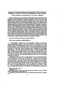
Fig. 1. A mixture of two bivariate wrapped normal distributions shown as a heatmap. The two modes are shown in dark red. JOURNAL OF ADVANCES IN INFORMATION FUSION

VOL. 11, NO. 2

DECEMBER 2016

hypersphere S d , which is the surface of the unit ball in Rd+1 . The other important topology is the Cartesian product of multiple circles S 1 £ ¢ ¢ ¢ £ S 1 called hypertorus, which will be the focus of this paper. The hypertorus is the proper topology to use when dealing with multiple, possibly stochastically dependent angles in the range of [0, 2¼). Examples featuring a hypertoroidal topology include angles at different points in time or connected rotatory robotic joints. If the variates of the random vector are stochastically independent, they can be treated as independent random variables and filters for circular topologies can be used. For the circle, several filters have been proposed [17], [18], [19], [20], [21], [22]. However, filters for multivariate angular problems are necessary if the random vector cannot be separated into multiple independent random variables. For example, if the random variables x and y are independent, the two variates of the vector [x x + y]T are (usually, but not necessarily) dependent. They can, however, be easily transformed into a problem featuring independent variates that can be estimated independently. The obtained estimates can then be transformed back for use in the original problem featuring dependent variates. In practice, transforming the problem in a way that causes the components to be independent is usually nontrivial and frequently impossible. On linear domains, an important filter is the Kalman filter that scales well with increasing number of variates and yields optimal estimation results if certain conditions are met. The Kalman filter can handle correlations and scales no more than cubically in the number of variates. For nonlinear system or measurement models, such an efficient and optimal solution does not exist in general. Therefore, even on linear domains, nonlinear estimation is a challenging task, especially for multivariate problems. On periodic domains, estimation problems are inherently nonlinear and thus challenging to deal with for higher numbers of variates. For multivariate angular estimation, a recursive filter has been suggested in [23] for the two-dimensional torus. However, due to the approximation with a single bivariate wrapped normal distribution, multimodal bivariate posteriors, such as the one shown in Fig. 1, cannot be modeled adequately. As an alternative for toroidal and hypertoroidal estimation problems, the very general concept of a sampling importance resampling (SIR) particle filter [24] that is popular on linear domains can be adapted in a straightforward manner to periodic manifolds. In this paper, we generalize a recursive Bayesian estimator based on Fourier series, which we proposed for univariate densities on the circle in [21]. Our new approach to multivariate angular estimation problems on the hypertorus is based on representing the density or its square root using a multidimensional Fourier series. Based on the representation used, we either call the filter the (angular) Fourier identity filter or the (angular)

Fourier square root filter and we abbreviate their names as IFF and SqFF. We show that the prediction and filter operations can be performed in computationally efficient ways, never exceeding an asymptotic complexity of O(n log n) for n Fourier coefficients and a fixed number of variates. However, for estimation problems with a higher number of variates, it is advisable to use more Fourier coefficients. The rest of this paper is structured as follows. We give a brief explanation on how to perform recursive Bayesian estimation in general and lay out the required operations in the next section. We introduce the basics of Fourier series and directional statistics that are a prerequisite for our proposed approach in the third and fourth section. In the fifth section, we address related work and explicate the key idea of our proposed filters. In Sec. VI, we introduce an actual implementation of the Fourier filters. A comparison of our proposed filters and an evaluation comparing the Fourier filters with other approaches is given in Sec. VII. A conclusion and an outlook is provided in Sec. VIII. Finally, we present some useful properties of the Fourier series representations in the appendix. II.

RECURSIVE BAYESIAN ESTIMATION

While a lot of effort in estimation theory is geared towards estimating the mean of the posterior density, keeping track of the whole density is usually required for accurate results over multiple time steps. The focus on approximating the mean can be explained by the fact that on linear domains, the mean of the posterior density is the minimum mean squared error estimator [25, Sec. 10.3]. However, if the density is to be reused in future time steps, the mean of the posterior density itself does in general not suffice for an accurate calculation of the mean of the posterior density in future time steps. In the case of linear systems with Gaussian noise on linear domains, keeping track of the whole density is easy– the resulting Gaussian posterior density is precisely described by the mean vector and the covariance matrix. For noise terms that are not exactly Gaussian distributed and especially for nonlinear models, describing the precise posterior density using a limited number of parameters is challenging or impossible even on linear domains. Many estimators focus on approximating the posterior density using a parameterized density of a prespecified family of densities. For example, Gaussian assumed density filters [26], [27], [28], [29] try to find a suitable Gaussian approximation for the true posterior density. To increase the accuracy of the approximation, Gaussian mixtures [26] can be used but mixtures entail further problems concerning component reduction [30]. Another popular approach is to use an SIR particle filter [24]. While simple particle filters can be used to asymptotically approximate moments such as the mean over multiple time steps, they are non-deterministic and do not directly provide a continuous approximation of the density.

MULTIVARIATE ANGULAR FILTERING USING FOURIER SERIES

207

In the subsections of this section, we introduce the general formulae that can be used for recursive Bayesian estimation with given likelihoods and transition densities and lay out the required operations for implementing a recursive Bayesian estimator. The formulae presented are suitable for manifolds with a topological group structure, such as Rn and the hypertorus. A. Prediction Step The prediction step can be described by the Chapman— Kolmogorov equation p ft+1 (x t+1 j z 1 , : : : , z t ) Z = ftT (x t+1 j x t )fte (x t j z 1 , : : : , z t )dx t , −x

in which −x denotes the sample space–for hypertori, [0, 2¼)d –ftT the transition density, fte the posterior denp sity, and ft+1 the prior density based on measurements up to the time step t. For identity models involving additive noise on linear domains, we can write x t+1 = x t + w t ,

(1)

with wt distributed according to ftw . On periodic domains, this becomes x t+1 = (x t + w t ) mod 2¼, which includes a nonlinear transformation. In the case p of additive noise, we can simplify the formula for ft+1 to p (x t+1 j z 1 , : : : , z t ) ft+1 Z = ftw (x t+1 ¡ x t )fte (x t j z 1 , : : : , z t )dx t −x

= (ftw ¤ fte )(x t+1 ) for both linear and circular domains and are able to perform the prediction step by calculating a continuous convolution. B. Filter Step If we obtain a measurement and know the corresponding measurement likelihood, we can use Bayes’ formula for the filter step. This essential concept can be formulated as fte (x t j z 1 , : : : , z t ) = R

ftL (z t j x t )ftp (x t j z 1 , : : : , z t¡1 ) p L −x ft (z t j x t )ft (x t j z 1 , : : : , z t¡1 )dx t L

p

/ ft (z t j x t )ft (x t j z 1 , : : : , z t¡1 ), with the likelihood function ftL . It is important to note that the denominator is independent of x t and can thus be treated as a constant. Since we know that a proper pdf integrates to one, we can ignore the denominator if we have other means to normalize the density. III. BASICS OF DIRECTIONAL STATISTICS In this section, we introduce important concepts of directional statistics. In directional statistics, there are 208

counterparts to many important concepts used in the context of linear domains, some of which are addressed in this section. We always assume that our periodic region has a size of 2¼ along each dimension. While most formulae given in this paper do not explicitly depend on the precise region used, we say that our periodic quantities are always in [0, 2¼) in the scalar case and in [0, 2¼)d in the d-variate case. In this paper, we use the von Mises distribution as well as the wrapped normal distribution and generalize the latter to an arbitrary number of variates. We chose to use the multivariate wrapped normal distribution as it can be trivially generalized from its bivariate definition. Another important concept is that of trigonometric moments. While these moments are seldom used on linear domains, they are a useful concept to employ instead of power moments when dealing with periodic densities. We also introduce concepts for describing correlations between the variates of a random vector on hypertoroidal manifolds. For further reading, we recommend the two classic books about directional statistics [10], [11]. A. Von Mises Distribution The von Mises distribution [10, Sec. 3.5], also called the circular normal distribution [11, Sec. 2.2.4], is a popular circular distribution. A useful property of this distribution is that the product of two von Mises distributions yields an (unnormalized) von Mises distribution again. The density of the von Mises distribution is given by e·cos(x¡¹) fVM (x; ¹, ·) = , 2¼I0 (·) with I0 (¢) being the modified Bessel function of the first kind, ¹ 2 [0, 2¼) being the location parameter, and · ¸ 0 describing its concentration. B. Wrapped Normal Distribution The wrapped normal distribution [10, Sec. 3.5] can be, visually speaking, obtained by wrapping a Gaussian distribution around the circle and summing up all probability mass at each point. The density is defined as X fWN (x; ¹, ¾ 2 ) = N (x + 2¼j; ¹, ¾2 ), j2Z

in which we parameterize the density based on the mean ¹ 2 [0, 2¼) and the variance ¾ 2 of the underlying normal distribution. We use the variance instead of the standard deviation to provide a definition that is consistent with the multivariate case introduced in the next subsection. C.

Multivariate Wrapped Normal Distribution

The concept of a wrapped normal distribution can be generalized to higher dimensions, e.g., to the torus as a bivariate wrapped normal (also called wrapped bivariate normal) distribution [11, Sec. 2.3.2]. For the d-variate wrapped normal distribution, we wrap a

JOURNAL OF ADVANCES IN INFORMATION FUSION

VOL. 11, NO. 2

DECEMBER 2016

d-variate normal distribution onto the d-dimensional hypertorus. This leads to the formula X fWN (x; ¹, CWN ) = N (x + 2¼j;¹, CWN ) j2Zd

for the density of the d-variate distribution with the vector-valued mean ¹ 2 [0, 2¼)d and covariance matrix CWN . D. Trigonometric Moments One important concept on linear domains are power moments, usually simply referred to as moments. Moments describe useful properties of the distribution and are important for estimators. As previously mentioned, the first moment of the posterior density is the MMSE estimator on linear domains. Distributions of certain types can be parametrized by some of their moments, e.g., for the Gaussian distribution, the combination of the first moment and the second central moment (or its root) is the most commonly used parameterization. On periodic manifolds, trigonometric (also called raw) moments feature some of the properties that power moments have on linear domains. The kth trigonometric moment (k 2 N) for scalar random variables is given by [11, Sec. 2.1] Z 2¼ ikx f(x)eikx dx: mk = E(e ) = 0

It is also common practice to write trigonometric moments as vectors instead of as a complex number. For this representation, used for example in [10, Sec. 3.4.1], the parts represented by the real and imaginary part are calculated using separate integrals. However, using Euler’s formula, it can be shown that the conversion from one representation to the other is straightforward. Unlike power moments, trigonometric moments consist of two values–either the real and complex parts or the two components of the vector–and thus, a single moment can describe multiple properties. For example, the first trigonometric moment is not only a measure of the density’s position but also of its dispersion. The parameters for some distributions, such as the wrapped normal and the von Mises distribution, can be derived from the first trigonometric moment [18]. As trigonometric moments express a lot about the density, several filters in the circular case approximate trigonometric moments and make use of them. Due to the close relationship of some of the Fourier coefficients to trigonometric moments, the Fourier filters are no exception. For the kth moment of multivariate densities, we simply stack all kth moments of all variates. Thus, in

the d-variate case, the kth moment is given by 3 2R ikx1 2m 3 2 ikx1 3 dx E(e ) [0,2¼)d f(x)e k,1 R 7 ikx2 6 m 7 6 E(eikx2 ) 7 6 dx 7 6 k,2 7 6 7 6 [0,2¼)d f(x)e 7 6 7 6 7=6 mk = 6 7: .. 6 .. 7 = 6 7 6 . 7 .. 4 . 5 4 5 4 . 5 R ikxd ikx E(e ) mk,d d dx [0,2¼)d f(x)e (2) E. Circular Mean Direction The circular mean direction, which can be thought of as an analogue to the linear mean, only describes the density’s location and can be calculated from the first trigonometric moment via [10, Sec. 2.2] ¹ = atan2(I(m1 ), R(m1 )):

(3)

A useful property on linear domains is the linearity of the expected value, which does not hold for the circular mean direction [11, Sec. 2.2.1]. For the circular mean direction in the d-variate case, we simply calculate the circular mean direction for every component of the moment vector according to (3), yielding 2 3 atan2(I(m1,1 ), R(m1,1 )) 6 7 .. 7: ¹=6 4 5 . atan2(I(m1,d ), R(m1,d ))

F. Angular Correlation Coefficients A variety of measures of correlation of two angular random variables have been introduced in the literature. Examples include the correlation coefficients by Jammalamadaka and Sarma [31], Johnson and Wehrley [32], and Jupp and Mardia [33]. One of the correlation coefficients is used by the only assumed density filter for bivariate toroidal problems [23] that we know of. As shown in Appendix D, a limited number of Fourier coefficients contain all information necessary to calculate all correlation coefficients mentioned. Key to this is the close relationship of the correlation coefficients to a certain covariance matrix. In the bivariate case, all of these correlation coefficients can be calculated using entries of the covariance matrix 002 1 02 1T 1 3 3 cos(x1 ) cos(x1 ) BB6 C B6 sin(x ) 7 C C BB6 sin(x1 ) 7 C B6 C C 7 1 7 § = EB ¡ ¹ ¡ ¹ 6 C B 6 C C 7 7 BB c A @4 cA C cos(x2 ) 5 @@4 cos(x2 ) 5 A sin(x2 ) sin(x2 ) with ¹ c = E([cos(x1 )

sin(x1 )

cos(x2 )

sin(x2 )]T ),

which can be calculated via ¹ c = [R(m1,1 ) I(m1,1 ) R(m1,2 ) I(m1,2 )]T : Thus, efficient calculation of this matrix allows efficient calculation of all correlation coefficients. It is easy to


209

extend this covariance matrix to arbitrary multivariate distributions by stacking the terms for all individual variates, yielding 002 3 3 1 02 1T 1 cos(x1 ) cos(x1 ) BB6 C B6 sin(x ) 7 C C BB6 sin(x1 ) 7 7 C B6 C C 1 7 BB6 7 7 C B6 C C BB6 7 7 C B6 C C . . B . . § = E BB6 7 ¡ ¹ c C B6 7 ¡ ¹ cC C . . 6 7 7 C B6 C C BB 6 7 7 C B6 C C BB A @4 cos(xd ) 5 A C A @@4 cos(xd ) 5 sin(xd ) sin(xd ) with ¹ c = E([cos(x1 )

sin(x1 ) ¢ ¢ ¢ cos(xd )

sin(xd )]T ):

IV. BASICS OF FOURIER SERIES In this section, we give a brief introduction to multidimensional Fourier series, the second concept essential to this paper. For details regarding Fourier series, we refer the reader to the two-volume book series about trigonometric series by Zygmund [34] and books about harmonic analysis [35]. A. One-Dimensional Fourier Series Using Fourier series, it is possible to approximate functions on [0, 2¼) using complex exponential functions. The set of functions ikx

fe

j k 2 Zg

is an orthogonal basis that can be used to represent any square-integrable (also called square-summable) complex function defined on [0, 2¼) using a squaresummable sequence of Fourier coefficients [35, Sec. I5]. Since densities encountered in practice are usually square-integrable, we can write their density f(x) as a Fourier series 1 X f(x) = ck eikx , (4) k=¡1

where the Fourier coefficients ck 2 C fulfill X jck j2 < 1: k2Z

The Fourier coefficients can be calculated from the density according to Z 2¼ 1 f(x)e¡ikx dx: ck = 2¼ 0 For real functions, c¡k = c¯ k holds [34, Ch. I], causing imaginary parts to cancel out in (4). Furthermore, it is also possible to use real basis functions and coefficients to represent real functions. In this alternative representation, the series in (4) becomes a weighted sum of sine and cosine functions of different frequencies. B. Higher-Dimensional Fourier Series The straightforward generalization of one-dimensional Fourier series to the d-dimensional case is to use 210

functions of the orthogonal system fei(k1 x1 +k2 x2 +¢¢¢+kd xd ) j k 2 Zd g to represent functions on the d-dimensional hypercube [34, Ch. XVII] (or in our case hypertorus) [0, 2¼)d . In the following, we write the basis functions described above using a dot product as eik¢x and use a vectorvalued index k 2 Zd to specify individual entries ck of the d-dimensional Fourier coefficient tensor. Using this notation, a multidimensional Fourier series can be X written as ck eik¢x : f(x) = k2Zd

The individual Fourier coefficients can then be calculated via Z 1 ck = f(x)e¡ik¢x dx: (5) (2¼)d [0,2¼)d In this paper, our focus is on Fourier series for which only n specific coefficients are nonzero and we only consider sets of indices J that are subsets of the integer lattice Zd with an equal subset of Z in each dimension. If every subset of Z ranges from ¡kmax to kmax in each dimension, the total number of Fourier coefficients is n = (2kmax + 1)d . Similar to the one-dimensional case, c¡k = c¯ k holds for real functions. REMARK 1. The formulae for the Fourier coefficients bear a close resemblance to the trigonometric moments. The kth trigonometric moment m k can be calculated from the Fourier coefficients via m k = (2¼)d [c¡k,0,:::,0

c0,¡k,0,:::,0 ¢ ¢ ¢ c0,:::,0,¡k ]T :

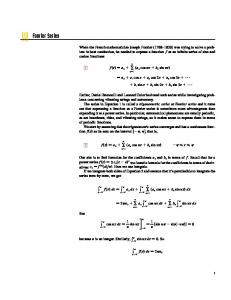
Thus, all trigonometric moments and especially the first trigonometric moment required for the calculation of the circular mean direction can be calculated efficiently from the Fourier coefficients. On the other hand, calculating arbitrary Fourier coefficients from the trigonometric moments is, in general, only possible in the onedimensional case. For higher dimensions, many entries of the Fourier coefficient tensor do not have corresponding entries in the moment vectors as defined in (2). We visualize this for the two-dimensional case in Fig. 2. In Appendix D, we show that there is a relationship between the covariance matrix described in Sec. III-F and other entries of the Fourier coefficient tensor. V.

RELATED WORK AND KEY IDEA

For our approach, it is important to note that many important multivariate densities–such as the multivariate wrapped normal density–are square-integrable and thus lend themselves well to approximations using Fourier series. Mardia also states this observation for the univariate case in his book [10, Ch. 3—4], noting that if the Fourier coefficients are square-summable, the corresponding density is equal to the Fourier series almost everywhere. Willsky discusses optimal filtering using nontruncated Fourier series with an infinite number of co-


VOL. 11, NO. 2

DECEMBER 2016

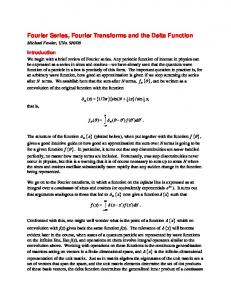
Fig. 3. Different representations that are used by the filters.

holds. Therefore, the Fourier coefficients are squaresummable and thus converge to zero, facilitating the approximation via a Fourier series. Furthermore, if gk max denotes the truncated Fourier series respecting the coefficients from ¡kmax to kmax , the convergence of gk

max

Fig. 2. Visualization of the relationship between the Fourier coefficients and the trigonometric moments of a bivariate distribution. Fourier coefficients that are unrelated to all trigonometric moments are shown in blue, coefficients that are related to the first entry of a trigonometric moment vector are shown in green, and coefficients that are related to the second entry are shown in yellow. The zeroth coefficient in the middle determines both entries of the zeroth trigonometric moment vector and is identical for all (normalized) densities.

efficients in [6]. Since infinite series cannot be handled computationally, he discusses practical implementations in [16]. Willsky deems the performance of a filter working with truncated Fourier series to be insufficient for few coefficients and suggests making the assumption that the density is distributed according to a wrapped normal distribution, which we believe is too restrictive. Ferna´ ndez-Dura´ n [36] observes that when approximating densities using Fourier series, the truncation of the coefficient vector can cause negative function values and suggests a computationally expensive way to ensure nonnegativity. In the context of nonlinear filtering for linear domains, Brunn et al. [37], [38] argue that approximating a transformed version of the pdf allows the reconstruction of a valid density with only nonnegative values in every time step. Based on this idea, we have presented a filter for univariate periodic densities in [21] that ensures the validity of a density function f : [0, 2¼) ! R+ 0 by approximating the square root of p the density. Approximating the square root g(x) = f(x) of the density is reasonable as the square root of every density is square-integrable since Z Z g(x)2 dx = f(x)dx = 1 [0,2¼)

[0,2¼)

kmax !1 p

¡!

f also implies gk2

max

kmax !1

¡! f

almost everywhere. For this representation, we showed in [21] how prediction and filter steps can be calculated efficiently and accurately using the Fourier coefficients for univariate estimation problems. In a scenario featuring bimodality, the filter presented outperformed both a grid filter and a particle filter. In this paper, we generalize the approach presented in [21] to higher dimensions and approximate multivariate periodic densities or their square root using multidimensional Fourier series. Based on these approximations, we describe how the prediction and filter steps of a recursive Bayesian estimator can be calculated efficiently in the multivariate case. Since run time is crucial for high numbers of variates, we put emphasis on comparing configurations of equal run time. Furthermore, we closely regard the IFF, which has disadvantages in theory but features a lower run time when using an identical number of coefficients. VI. RECURSIVE BAYESIAN ESTIMATION BASED ON FOURIER SERIES In this section, we present how a recursive Bayesian estimator can be implemented based on approximating the density or its square root using a Fourier series. For the SqFF, we are dealing with a total of four representations that can be used to obtain values of the probability density (see Fig. 3). These include the original function, the Fourier coefficients of the original function, the square root of the function, and the Fourier coefficients thereof. Only the first two representations are used in the IFF. Deriving a Fourier series representation for a function is commonly referred to as Fourier analysis whereas reconstructing the function is frequently called Fourier synthesis. As the different representations have implications for the algorithmic implementation of the operations, we will make a clear notational distinction between Fourier coefficient tensors representing the actual density Cid and coefficient tensors representing the


211

square root of the density Csqrt and apply the same notation to the individual entries of the tensors denoted by ckid and cksqrt with the vector-valued index k. For the upper two representations in Fig. 3, there are important dualities that we make use of. The convolution of two functions corresponds to a Hadamard (entrywise) product of their Fourier coefficient tensors. Furthermore, the multiplication of two functions represented as a d-dimensional Fourier series can be performed using a d-dimensional discrete convolution of the coefficient tensors. In order to perform (or at least approximate) the prediction and filter steps described in Sec. II, we first need to be able to transform arbitrary densities and likelihoods into the two Fourier series representations. Second, we need to be able to perform multiplications and normalizations for the filter step in the respective representation. Third, convolutions are necessary to perform prediction steps for an identity model with additive noise (1). While exact results for both operations can be obtained in the IFF, an increase in the number of coefficients would be inevitable. While we may allow the number of coefficients to vary over time, parameter reduction becomes inevitable in the long run. Parameter reduction generally induces an approximation and is also necessary for the SqFF. For our implementation of the filters, we do not allow the number of coefficients to vary over time and truncate to an identical number of coefficients after each prediction and filter step. In the following, we describe how the filter step, the prediction step, and the parameter reduction can be performed in O(n log n) for n Fourier coefficients. Further properties that are useful to applying the filter in practice but are not essential to the filter and prediction step are given in the appendix. A. Transforming Multivariate Densities An efficient approach to Fourier analysis was proposed by Cooley and Tukey [39]. This approach has become widespread for calculating the closely related discrete Fourier transform [40, Ch. 2] and is nowadays known as the fast Fourier transform (FFT) [41], which is also how we will refer to it and its higher-dimensional generalizations for the remainder of this paper. The complexity of the FFT is O(n log n) for a total number of n coefficients. However, for a fixed kmax , the number of coefficients still grows exponentially with the dimensionality of the space. This is not a serious problem for low numbers of variates and we have verified good filter results with fast run times for densities with up to five variates. To obtain a Fourier series approximation of the square root of a density using the FFT, there is (aside from calculating the square root of each function value) no additional overhead involved. In the one-dimensional case, we were able to derive closed-form formulae for the coefficients for many important univariate densities [21]. In Appendix A of this 212

paper, we provide the formula for the Fourier coefficients of the multivariate wrapped normal distribution. While closed-form formulae can lead to lower run times, the cost of calculating n coefficients is always at best in O(n) when at least n coefficients are required for an exact representation of the density. For identity system and measurement models with independent, time-invariant additive noise terms, we can reduce the computational effort involved in obtaining the required Fourier coefficients. In these cases, it is not necessary to transform the density of the system noise and the likelihood in each time step. The density of the system noise simply stays identical while the likelihood is only influenced by the measurement via a shift. For example, for an additive system noise that is distributed according to a multivariate wrapped normal distribution, the density of the system noise is ftw (w t ) = fWN (w t ; ¹, CWN ) in every time step. Similarly, we can avoid the need for transforming the likelihood multiple times for additive noise terms. If the likelihood is ftL (z t j x t ) = fWN (z t ; x t , CWN ) = fWN (x t ; z t , CWN ) we can initially transform the likelihood when setting z = 0 (meaning, fWN (x; 0, CWN ) in our case) and then calculate the Fourier coefficients of the actual likelihood respecting the current measurement z t from these coefficients. The individual Fourier coefficients ckshifted for a function shifted by z can be calculated according to ckshifted = ck e¡ik¢z ,

(6)

which is a straightforward generalization of the shifting operation for the scalar case (Theorem 1.1 (iv) in [34, Sec. II-1]). B. Filter Step To implement the filter step, two operations have to be performed for the two filters. The first operation is a multiplication of the prior density ftp (x t j z 1 , : : : , z t¡1 ) and the likelihood ftL (z t j x t ). The coefficient tensors for the intermediate, unnormalized results will be called ³ e,sqrt . In the second step, the densities are ³ e,id and C C t t and normalized to yield the coefficient tensors Ce,id t Ce,sqrt to be used in the next prediction (or filter) step. t The filter steps for the two Fourier filters are illustrated in Fig. 4 and the necessary operations are explained in detail in the following. 1) Multiplication of Two Densities: The first operation necessary to perform the filter step of our Bayesian filter is the multiplication operation. Let us now denote the Fourier coefficient tensor of ftp (x t j z 1 , : : : , z t¡1 ) as Cp,id t and refer to the Fourier coefficient tensor of ftL (z t j x t ) (for a fixed measurement z t , depending only on the state x t ) as CL,id t . For the IFF, we can then directly obtain


VOL. 11, NO. 2

DECEMBER 2016

coefficients can be converted (pairwise) into sine and cosine functions of differing (but nonzero) frequencies using Euler’s formula. Integrating these trigonometric functions over [0, 2¼) always yields zero. Therefore, the integral over the whole function can be calculated according to Z Z X id ik¢x id id ³ct,k ³ct,0 e dx = dx = (2¼)d ³ct,0 [0,2¼)d

Fig. 4. Filter step of the IFF and the SqFF. (a) Illustration of the filter step of the IFF. (b) Illustration of the filter step of the SqFF.

³ e,id for the new Fourier series the coefficient tensor C t representing the unnormalized multiplication of the two functions via ³ e,id = Cp,id ¤ CL,id , C t t t in which ¤ denotes the discrete convolution. The discrete convolution can be performed in O(n log n) using FFT-based convolution approaches or by using alternative convolutions methods tailored to the multidimensional tensor convolution [42]. Since the discrete convolution of two tensors results in a larger tensor, parameter reduction as explained in Sec. VI-C becomes necessary. The multiplication can be performed similarly for the SqFF. Owing to the fact that for all functions ftp (x t j z 1 , : : : , z t¡1 ) and ftL (z t j x t ) and for all vectors x t and z t in the respective domains q q ftp (x t j z 1 , : : : , z t¡1 ) ¢ ftL (z t j x t ) q = ftp (x t j z 1 , : : : , z t¡1 )ftL (z t j x t ) holds, we can simply multiply the functions in the square root representation. Thus, the multiplication can be performed analogously to q the IFF. For the Fourier

of ftp (x t j z 1 , : : : , z t¡1 ) and coefficient tensors Cp,sqrt t p of ftL (z t j x t ) (again, for a fixed measurement), CL,sqrt t we can calculate the unnormalized coefficient tensor ³ e,sqrt in the square root representation using C t ³ e,sqrt = Cp,sqrt ¤ CL,sqrt : C t t t 2) Normalization: The second operation necessary for the filter step is the normalization. We use ³ct,k to refer to an entry of the coefficient tensor to be nor³ e,sqrt as obtained from the ³ e,id or C malized, such as C t t multiplication above. For the normalization, we need to integrate over the whole domain of the function, which is easy when a Fourier series is used to represent a real function. In the integral, all terms except the one stemming from the first coefficient integrate to zero. This is obvious since the exponential functions for all other

[0,2¼)d

k2Zd

in the non-rooted representation. Thus, we can normalid ize the density by dividing all coefficients by (2¼)d ³ct,0 , which ensures that the coefficient with index 0 of the id new, normalized density is ct,0 = 1=(2¼)d . For the square root version, we can calculate the integral of the function by determining the Fourier coefficient with index 0 of the non-rooted representation. id can be calculated from the coeffiThe coefficient ³ct,0 sqrt cients ³ct,k of the square root representation via X sqrt sqrt X sqrt id ³ct,k ³ct,¡k = ³ct,0 = j³ct,k j2 : k2J

k2J

Based on this insight, we can ensure that the density represented by the Fourier series integrates to one by q P sqrt d ³sqrt 2 dividing all ³ct,k by (2¼) k2J jct,k j . Since calculating the sum of the square of the absolute values is in O(n) and the division of all coefficients is also in O(n), normalization is possible in O(n) for both representations. C.

Parameter Reduction

The need for parameter reduction in the Fourier filters is reminiscent of nonlinear filters on linear domains. Except for very simple problems, representing the exact result of both convolution and multiplication operations usually results in an increase in the number of parameters. In the long run, parameter reduction becomes necessary and usually requires approximations. A popular example of nonlinear estimators are estimators based on Gaussian mixtures. For mixtures, component reduction is a non-trivial and expensive operation, in which the density has to be approximated using a lower number of components while preserving the shape of the density as well as possible [30]. Parameter reduction is also essential for our proposed approach using Fourier series. As described in Sec. VI-B.1, the multiplication operation requires calculating a discrete convolution of the coefficient tensors, resulting in an increase in the size of the tensor. As common densities and especially their square roots are square-integrable, the coefficients tend to zero in every dimension. Therefore, the influence of the coefficients on the shape of the function converges to zero for increasing kkk and it is thus reasonable to use truncation as an easy way for parameter reduction. As can be seen in Sec. VI-B.2, renormalization is necessary after truncation for the SqFF as the integral


213

Fig. 5. Prediction step of the IFF.

depends on the sum of the squared absolute values of the coefficients. For the IFF, the integral only depends id on ct,0 and renormalization is thus not required. D. Prediction Step To perform the prediction step for an identity system model with additive noise (1), we only need to be able to convolve two densities. Convolving two functions using their Fourier coefficient tensors is possible very efficiently as this only involves a Hadamard product. The prediction step for nonlinear system models usually requires more than a convolution operation. An approach for arbitrary transition densities that can easily be extended to the multivariate case is laid out in [43]. 1) Prediction Step of the IFF: As illustrated in Fig. 5, we can directly use the rule for the convolution of two functions to obtain the Fourier coefficient tensor of the result. If Ce,id and Cw,id are the truncated Fourier t t coefficient tensors of fte (x t j z 1 , : : : , z t ) and ftw (¢), we can obtain the coefficient tensor Cp,id t+1 for p ft+1 (x t+1 j z 1 , : : : , z t ) = (fte ¤ ftw )(x t+1 )

via the use of the Hadamard product ¯ according to e,id ¯ Cw,id : Cp,id t t+1 = Ct

2) Prediction Step of the SqFF: Matters are more complicated when aiming to obtain the coefficient tensor Cp,sqrt representing the square root of the convolution t of the densities. Since we intend to obtain the Fourier coefficients for q p p ft+1 (x t+1 j z 1 , : : : , z t ) = (fte ¤ ftw )(x t+1 ), we cannot simply use the Hadamard product of the coefficient tensors Cp,sqrt and Cw,sqrt as this would yield t t the coefficient tensor for the Fourier series representing q p fte (x t j z 1 , : : : , z t ) ¤ ftw (¢), which is, in general, unequal to p (fte ¤ ftw )(x t+1 ): Instead, we first calculate the Fourier coefficient tensor for (fte ¤ ftw )(x t+1 ) and then determine the coefficients of the square root, which we lay out in the following and illustrate in Fig. 6. First, we derive the Fourier coefficients for the non-rooted densities fte (x t j z 1 , : : : , z t ) 214

Fig. 6. Prediction step of the SqFF. The colors indicate the respective representation as laid out in Fig. 3.

and ftw (¢) from the square root representations. These ˜ w,id to ˜ e,id and C coefficient tensors are denoted by C t t emphasize that they contain more coefficients than the and Cw,sqrt . We can use original coefficient tensors Ce,sqrt t t the multiplication explained in Sec. VI-B.1 to derive the formulae ˜ e,id = Ce,sqrt ¤ Ce,sqrt C t t t

˜ w,id = Cw,sqrt ¤ Cw,sqrt : and C t t t

Based on this, we can use the discrete convolution to ˜ p,id for f p (x obtain the Fourier coefficient tensor C t+1 t+1 t+1 j z 1 , : : : , z t ) via ˜ e,id ¯ C ˜ w,id : ˜ p,id = C C t+1

t

t

As the next step, we wish to obtain the Fourier coefficient tensor for the square root representation with a specified number of coefficients. For this, we first p (x t+1 j z 1 , : : : , z t ) on calculate n function values of ft+1 an equidistant grid, take the square root these function values, and then use the FFT to obtain the Fourier coefficient tensor. To obtain the function values on an equidistant grid, we could now naïvely evaluate the ˜ p,id on all n grid Fourier series with coefficient tensor C t+1 points. However, to achieve a good run time behavior, we have to keep one more issue in mind. Unless there is a reason to do otherwise, it is reasonable that the number of coefficients to calculate for the result is linearly dependent on the number of coefficients used in the ˜ p,id . Since each function evaluation coefficient tensor C t+1 is in O(n), n function evaluations would be in O(n2 ). Therefore, it is significantly cheaper to use the inverse


VOL. 11, NO. 2

DECEMBER 2016

FFT with a complexity of O(n log n) to calculate the required n function values. p (x t+1 j z 1 , : : : , z t ) at With the function values of ft+1 our disposal, we can calculate theqsquare root of each

p value to obtain n function values of ft+1 (x t+1 j z 1 , : : : , z t ). These function values can then to be used to approximate n Fourier coefficients via the FFT. Since the most expensive operations are the inverse FFT, the FFT, and the discrete convolution, all of which are in O(n log n), the total effort is in O(n log n). In the step of calculating the square root, approximation errors are caused because taking the square root induces higher frequencies that are not accounted for. Furthermore, as the discrete convolutions used in the ˜ w,id result in an increase in the ˜ e,id and C calculation of C t t number of coefficients, we need to perform parameter reduction if the coefficients should not be allowed to increase with every prediction step. The parameter reduction can be performed as described in Sec. VI-C. Afterward, a normalization step is required due to the approximations performed.

VII. EXPERIMENTS AND EVALUATION In this section, we compare our implementations of the two Fourier filters to each other and to other applicable filters. Both filters are available as part of libDirectional [44], a Matlab toolbox for directional statistics with a focus on recursive Bayesian estimation. In Sec. VII-A, we lay out theoretical benefits of the SqFF and describe an experiment to compare the filter steps of the Fourier filters in the univariate case. In the experiment, measurements are simulated regardless of how likely they are. This means we simulate both very likely measurements and unlikely measurements that we would rarely obtain if all underlying assumptions of the filter are correct. For all of these measurements, we evaluate the circular mean direction (3) and the approximation quality of the posterior density provided by the IFF and SqFF. In the second subsection, we evaluate the error in the form of an angular distance for the two Fourier filters in two bivariate scenarios and one trivariate scenario with additive, wrapped normally distributed noise terms and compare the results with those of other applicable filters in these scenarios. While there is a bivariate wrapped normal filter for toroidal manifolds [23], the only approach to the knowledge of the authors that is applicable to arbitrary multivariate angular estimation problems is the particle filter. Since the number of coefficients used by the Fourier filters and the number of particles used by the particle filter has a major impact on the filter performance, we evaluated several possible configurations. In the scenarios in the second subsection, the likelihoods to be used in each time step can be efficiently calculated using an initial transformation of the likelihood that is shifted according to the measurement obtained.

In the third subsection, we simulate an application of the filters to estimating the angles of a robotic arm based on measurements of the position of the end effector. This application shows that we can use our filter as long as we have a likelihood function and do not require a periodic measurement space. However, this scenario requires more computational effort for the Fourier filters as a Fourier series approximation of the likelihood has to be performed in each time step. Unlike our evaluation of the circular SqFF in [21], we do not regard the quality of the pdfs and cdfs for the multivariate cases. First, it is difficult to derive a continuous pdf from an SIR particle filter and comparing the cdf becomes increasingly difficult for higher dimensions, especially as a starting point of the integration has to be chosen on periodic domains. Second, we do not have any other filter to numerically approximate the ground truth with at our disposal. In our current evaluation, we also compare the run time of the filters and take the run times into account when assessing the individual filters. A. Comparing the IFF and the SqFF for Varying Measurements Allowing the function approximating the density to become negative has many inherent theoretic disadvantages as several useful concepts depend on valid pdfs.1 Based on an approximation of the pdf with negative function values, no valid cdf can be derived. Furthermore, sampling the density using equally weighted samples may not be possible and sampling schemes such as Metropolis—Hastings sampling [46] do not work. Moreover, some measures of similarity between two densities, such as the Kullback—Leibler divergence [47, Sec. 8.5] and the Hellinger distance [48], cannot be calculated due to the logarithm or square root involved. In most cases, we observed the approximation quality of the prior density or likelihood function to be already superior for the square root representation when compared with the non-rooted representation with an identical number of coefficients. An example of this is shown in Fig. 7. In the following, we regard the filter step of the Fourier filters and show how both filters perform when comparing the posterior densities and circular mean directions obtained. Even if no truncation is performed in the filter operations described in Sec. II-B, the approximation errors in the prior density and the likelihood function cause errors in the filter result. The severity of this effect strongly depends on the actual prior density and likelihood function. One important factor influencing the quality of the approximation of the posterior density 1 Negative probabilities [45] can be a viable tool as long as they only appear as intermediate results or if implications are made for other properties that are unobservable simultaneously in the context of physics. In our case, they have no special semantic but stem from approximation errors and have a negative impact on our estimator.


215

Fig. 7. Von Mises distribution with ¹ = ¼ and · = 10 and corresponding Fourier series approximations using 7 coefficients.

is the overlap of regions of high and low function values of the prior density and the likelihood function. To understand this effect, we have to take a closer look at the convergence of the Fourier series. A Fourier series converges in the L2 distance, which is a measure of the squared absolute deviation. Due to the close relationship between the L2 distance and the Hellinger distance, optimizing the L2 distance is reasonable when regarding one density individually. However, when regarding the product of two functions, one also has to regard the relative deviation to make statements about the quality of the approximation of the (normalized) multiplication result. Since the Fourier series converges regarding the absolute deviation and not regarding the relative deviation, we expect to see a higher relative deviation in regions of low density than in regions of high density. This has profound implications for the result of the multiplication of two functions. Let us assume both the prior density and the likelihood are unimodal and are close to zero except for values §¼=2 around their modes, such as the von Mises distribution with · = 10 that we show in Fig. 7. The prior distribution shall now have a mean of ¹ = 34 ¼ and the likelihood of ¹ = 32 ¼. Then, as can be seen in Fig. 8, the relative error of the approximation of the likelihood using 7 coefficients is very high in regions far from the mode, especially when approximating the function directly. When multiplying the prior with the likelihood, the small deviations visible in Fig. 7 are massively amplified in regions of high relative deviation of the likelihood (and also the other way around). This leads to a high deviation from the actual posterior in total. In this example, we can see that the approximation used in the SqFF is advantageous as the relative error is significantly less. However, there is another effect occurring in the filter step that strongly differs for the two filters. While it is possible to efficiently ensure that a density represented by its Fourier coefficients integrates to one both for the non-rooted and the square root representation (see Sec. VI-B.2), the underlying pdfs that are integrated differ substantially. For the square root representation, 216

Fig. 8. Approximations of the likelihood and the relative error of the approximations when using Fourier series with 7 coefficients. The likelihood follows a von Mises distribution with ¹ = 32 ¼ and · = 10.

the integral is over nonnegative values, whereas negative function values are possible for the non-rooted version. Always normalizing to one induces a higher total deviation from the abscissa for functions with negative parts as positive and negative parts cancel out. Furthermore, if more than half of the supposed density is negative, normalization to one causes negative parts to become positive and vice versa. In Fig. 9, we show the filter results for different distances between the modes when the prior density and the likelihood are von Mises distributions with · = 10. Both the prior density and the likelihood function were approximated using five Fourier coefficients for both filters and the Fourier series for the posterior densities were also truncated to five coefficients. Fig. 9a and Fig. 9b show the posterior density for the two filters when the modes of the prior density and likelihood function are ¼=2 apart. While the normalized result of the Fourier identity filter shows highly negative parts and has the lowest probability density around the peak of the true posterior, the main peak of the SqFF matches that of the true posterior. Furthermore, the result of the SqFF captures the circular mean direction of the posterior density correctly, while the IFF is off by ¼. Fig. 9c and Fig. 9d show the results when the modes of the two functions are almost ¼ apart. In this case, the true posterior is much flatter than the filter results that bear more of a resemblance to a mixture of the original densities. However, the mean is still correctly captured by the SqFF, while the IFF is off by ¼. In Fig. 10, we provide an evaluation depending on the distance ® between the two modes of the von Mises distributions. As the first criterion, we evaluate the quality of the posterior density. Since we are unable to use the Kullback—Leibler divergence and the Hellinger distance to compare the result of the IFF to the ground truth, we calculate the total variation [48] between the true densities and the filter results according to Z jh1 (x) ¡ h2 (x)jdx, d(h1 , h2 ) =


[0,2¼)

VOL. 11, NO. 2

DECEMBER 2016

Fig. 9. Examples for posterior densities provided by the two Fourier filters after a single filter step when using five coefficients. The circular mean directions of the posterior densities are shown as a vertical line in the respective color. (a) Result obtained using the IFF when the densities are at a distance of ¼=2. (b) Result obtained using the SqFF when the densities are at a distance of ¼=2. (c) Result obtained using the IFF when the densities are at a distance of almost ¼. (d) Result obtained using the SqFF when the densities are at a distance of almost ¼.

in which h1 = f1 f2 =kf1 f2 kL1 denotes the true density after the filter step and h2 is the result obtained by the respective variant of the filter. As the second criterion, we regard the quality of the point estimates. For this, we calculate the circular mean direction of the Fourier series approximation from the first trigonometric moment that can be easily obtained as described in Remark 1. Then, we calculate the shorter of the two arc lengths between the true circular mean direction ¯ and the circular mean direction of the filter result ° via [11, Ch. 1.3.2] dUV (¯, °) = min(¯ ¡ °, 2¼ ¡ (¯ ¡ °)):

(7)

A more in-depth discussion of metrics on the circle is given in [49, Sec. 2.2.2]. In the experiment, we limit ourselves to the range ® 2 [0, ¼ ¡ 0:01] as the true posterior for ® = ¼ is the wrapped uniform distribution that does not have a circular mean direction. The plots clearly show the sensitivity of the filters to larger distances between the modes. The two filters tend to perform worse for ® 2 [¼=2, ¼ ¡ 0:01] than for ® 2 [0, ¼=2] both regarding the circular mean direction and the total variation. Comparing the two filters with each other, the total variation between the filter result and the true posterior, as shown in Fig. 10a, can be seen to be higher in most cases when using the IFF. This was to be expected as negative function values are

possible for the result of the IFF. Both the negative parts and the highly positive parts required to cancel out the negative parts result in a higher total deviation. Therefore, deviations that are higher than the usual maximum of the total variation2 can be observed, e.g., in the case shown in Fig. 9a. The circular mean direction shown in Fig. 10b is correct for most distances between the means for both filters. This is because the circular mean direction of the result is calculated only from the first trigonometric moment, which is approximated well. Errors in the trigonometric moment usually occur over multiple time steps as an incorrectly shaped density is used for the next filter step, resulting in a wrong circular mean direction. However, as apparent in Fig. 10b, the circular mean direction can also become totally off in a single filter step. Using this criterion, the IFF is also more susceptible to errors than the SqFF. All in all, our results suggest that the SqFF is more robust when unlikely measurements are obtained. Furthermore, we can see that results obtained by the IFF can become totally unlike the true posterior density and can strongly violate the properties of valid densities. 2 The

total variation usually cannot exceed the value of two for valid densities.


217

were performed and the true states and the estimation results at each time step were saved for the calculation of our evaluation criterion. As the regarded scenarios feature multivariate estimation problems, we generalize the distance dUV given in (7) to a vector of angles ¯ and ° as v u d uX dMV (¯, °) = t (min(¯i ¡ °i , 2¼ ¡ (¯i ¡ °i )))2 : i=1

Fig. 10. Comparison of the performance of the IFF and the SqFF depending on the distance between the modes of the functions multiplied. (a) Total variation between the true posterior density and the densities obtained by the two filters. (b) Distance dUV between the true circular mean direction and the circular mean directions provided by the filters.

REMARK 2. Approximating the square root of the density is not the only option. However, using the square root ensures nonnegativity of the reconstructed density while necessitating only few approximations to maintain this representation. An alternative would be to use the logarithm, but the logarithm is highly nonlinear and especially regions with density values close to zero (in which the logarithm approaches ¡1) need to be treated with caution. Nonetheless, we plan to consider other transformations than the square root in future work. B. Evaluation of the Circular Mean Direction Having compared the two proposed Fourier filters for one filter step in the previous subsection, we now evaluate the Fourier filters against other state-of-theart approaches to multivariate angular filtering by comparing the estimation performance and run times when multiple filter and prediction steps are performed. In all scenarios, we initialized the filters using an approximation of the actual prior density used for the simulation. We have simulated the entire system behavior and the measurements for 50 time steps and performed alternating prediction and filter steps. A total of 1500 runs 218

This distance measure is similar to the Euclidean distance but takes periodicity into account. We calculate the distance between the ground truth vector and the estimate provided by the respective filter as a measure of the error of the estimator. To assess the estimation quality over all time steps and runs, we calculate the average of the errors over all time steps and all runs. Comparing the two Fourier filters regarding the average error is also an important part of our evaluation. While the results regarding the approximation of the density in the previous subsection were much more promising for the SqFF, the error in the circular mean direction was identical when the modes of the prior density and the likelihood function were close, which is a very common case. Furthermore, as the SqFF requires more convolution and FFT operations in the prediction step, the IFF can be used with more coefficients at an identical run time. Therefore, it is not obvious a priori which Fourier filter performs better when evaluating the average error for configurations of equal run time. All filters were implemented in Matlab without sophisticated optimizations and were compared on a laptop with an Intel Core i7-5500U processor, 12 GB of RAM, and Matlab 2016b running on Windows 10. The run times given are the average run times for each of the 50 time steps. For all filters, multiple different numbers of parameters were used. As kmax was chosen to be equal in every dimension, the numbers of parameters for the Fourier filter were always odd integers taken to the second (bivariate scenarios) or third (trivariate scenario) power. In all evaluations in this subsection, the likelihood at each time step can be obtained by shifting an initially transformed likelihood and this was used to reduce the effort necessary for the Fourier filters. In the following, we provide evaluation results for three scenarios. An identity model with additive noise (1) is used as the system and the measurement model in all scenarios. The first scenario features bivariate, unimodal transition densities and likelihood functions on the torus. The measurement and system noises are additive noise terms distributed according to multivariate wrapped normal distributions. This scenario is well suited for the use of the bivariate wrapped normal filter. The second scenario evaluated is also a bivariate scenario but features bimodal likelihoods instead of unimodal ones. The bimodality is introduced by using


VOL. 11, NO. 2

DECEMBER 2016

Fig. 11. Average errors and run times for the different filters in the bivariate scenario with unimodal likelihoods. (a) Error of the different filters depending on the number of particles or coefficients used. (b) Run times of the different filters for one time step depending on the number of particles or coefficients used.

Fig. 12. Average errors and run times for the different filters in the bivariate scenario with bimodal likelihoods. (a) Error of the different filters depending on the number of particles or coefficients used. (b) Run times of the different filters for one time step depending on the number of particles or coefficients used.

a mixture of two multivariate wrapped normal distributions at a distance of one radian in each dimension as additive measurement noise. Both mixture components are centered 0.5 radians away from the actual mean of the density along each axis. Approximating an arbitrary likelihood function using a (potentially unnormalized) wrapped normal distribution is no trivial matter and therefore we have not used the bivariate wrapped normal filter for this scenario and only compared our filters with the particle filter. The third scenario features trivariate densities on the three-dimensional hypertorus. The likelihoods are bimodal again and consist of two multivariate wrapped normal distributions at a distance of one radian in each dimension.

filters already appear to reach their optimal accuracy using approximately 100 coefficients, the particle filter does not yet achieve as good of an accuracy for thousands of particles. When taking the run times into account, the Fourier filters outperform the bivariate wrapped normal filter. The quality of the result of the bivariate wrapped normal filter can be surpassed with numbers of coefficients that still compare favorably in terms of the run time. While fast, the particle filter never comes close to the accuracy of the Fourier filters and the Fourier filters achieve better results using fast configurations with few coefficients. The IFF and the SqFF have almost identical estimation quality, but the IFF is faster. However, the filters achieve a quality that is close to its optimal estimation quality using only approximately 100 coefficients–a configuration at which the two filters differ only little in their run time.

1) Bivariate, Unimodal Scenario: The results shown in Fig. 11 confirm our intuition that the bivariate wrapped normal filter is well suited to this scenario. However, as the results of the Fourier filters show, the performance of the wrapped normal filter can be slightly exceeded by the Fourier filters that approximate the whole posterior density more accurately, facilitating better performance in future time steps. While the Fourier

2) Bivariate, Bimodal Scenario: In the results of this scenario, as shown in Fig. 12, the SqFF can be seen to provide better convergence when compared with


219

the IFF with identical numbers of coefficients. However, one can argue that the IFF is significantly faster and that, when comparing configurations with approximately equal run time, the IFF performs better than the SqFF. The results of the particle filter do not reach the accuracy of the Fourier filters even for high numbers of coefficients. The particle filter using over 2000 particles is outperformed by the SqFF with less than 500 coefficients in both accuracy and run time. Similarly, this holds for the IFF, whose estimation quality quickly surpasses that of the particle filter and which is significantly faster, resulting in a better performance for configurations with comparable run time. This scenario shows that the run time performance of the particle filter depends heavily on how fast the likelihood can be evaluated and even a mixture of two components instead of a single wrapped normal distribution can make a clear difference. For the Fourier filters, this does not hold for the identity model with additive noise as the likelihood is only transformed once and shifted afterward. 3) Trivariate, Bimodal Scenario: In the trivariate scenario, the possible configurations of the Fourier filters become more limited as we only use numbers of coefficients that can be written as an odd integer taken to the third power. However, as can be seen in Fig. 13, the superiority of the SqFF over the particle filter is evident. Its performance with corresponding numbers of parameters is better in terms of both the error and the run time, yielding a significant advantage when comparing configurations of comparable run time. Compared on a run time basis, the IFF also outperforms the particle filter since it can handle over 2000 coefficients with a run time that is lower than that of the particle filter with 200 particles. The bad run time performance of the particle filter is caused by the high computational effort required for evaluating the trivariate wrapped normal density used as the likelihood. As the number of variates increases, the effort involved in evaluating the wrapped normal distribution grows exponentially. To the knowledge of the authors, there is, in general, no other way to calculate the density of a wrapped normal distribution with an arbitrary number of variates other than to sum up some of the addends of the infinite sum. The number of addends required to approximate the density with sufficient accuracy increases exponentially with the number of variates. Thus, the particle filter not only requires more particles for an increasing number of variates, the evaluation of the likelihood also becomes exponentially more expensive. If the filter is used for a large number of time steps, the problem is far less severe for the Fourier filters. For an arbitrary number of time steps, the likelihood and the noise density only have to be approximated once if the likelihood is shifted in the computationally efficient way given in (6) in each time 220

Fig. 13. Average errors and run times for the different filters in the trivariate scenario with bimodal likelihoods. (a) Error of the different filters depending on the number of particles or coefficients used. (b) Run times of the different filters for one time step depending on the number of particles or coefficients used.

step. Therefore, the expensive likelihood only has to be evaluated on a grid once at the beginning. C.

Estimating the Joint Angles of a Robotic Arm In this subsection, we estimate the joint angles of a robotic arm based on measurements of the position of the end effector that are perturbed by multivariate Gaussian noise. Such a task could, e.g., arise when trying to validate the proper functionality of the robotic arm using external observations. The robotic arm, its joints, and the angles to be estimated are illustrated in Fig. 14. For simplicity, we assume that both joints can move freely and attain any angle. Only point measurements of the point in red on the end effector are obtained. As the end effector can only attain positions on a two-dimensional plane, the measurement is a vector comprising two components. To simplify the measurement equation, we set the zero coordinate of our coordinate system to the center of the first joint indicated in green in Fig. 14. Given the kinematics of the system, we obtain the measurement equation ¸ ¸ · · cos(®1 ) cos(®1 + ®2 ) h(®) = l1 + l2 sin(®1 ) sin(®1 + ®2 )


VOL. 11, NO. 2

DECEMBER 2016

Fig. 15. Likelihood when the measurement z t = [0 2:3]T m is obtained.

Fig. 14. Illustration of the robotic arm modeled in the simulation.

for ® = [®1 ®2 ]T . In our evaluation, we set the joint lengths l1 = 2 m and l2 = 1 m. To simulate sensor noise, the measurements are generated according to z t = h(® t ) + v t with a multivariate Gaussian distributed noise term v t » N (v; ¹, C) with the parameters · ¸ · ¸ 0 0:2 0 m and C = m2 : ¹= 0 0 0:2 While the measurement noise is uncorrelated in the measurement space, the likelihood function f L (z t j ® t ) = N (z t ;h(®t ), C) is, as shown in Fig. 15 for z t = [0 2:3]T m, asymmetric and the estimation problem thus cannot be trivially split up into univariate problems. Unlike in the previous subsection, the measurement equation is nonlinear and the likelihoods for differing measurements cannot be obtained by shifting an initial approximation of the likelihood. Therefore, a Fourier series approximation has to be performed in each time step, negatively affecting the run times of the Fourier filters. As the system model, we use a periodic analogue to a random walk model. This means ®t evolves according to ® t+1 = ® t + w t mod 2¼, with a time-invariant, multivariate wrapped normally distributed additive system noise term w t and a modulo operator that ensures that the angles are always between 0 and 2¼. The parameters ¹ and C of the system noise w t are identical to those of the measurement noise but the units are rad and rad2 instead of m and m2 . The scenario was simulated for 50 time steps with alternating filter and prediction steps. As in Sec. VII-B, we determine the error dMV in each time step and calculate the average over all 50 time steps and over 1500 runs. The results are depicted in Fig. 16 and are in line with the results obtained in the other bivariate scenarios. Both Fourier filters outperform the particle filter as configurations using only few coefficients provide better results than the particle filter using 2000 particles.

Fig. 16. Average errors and run times for the different filters in the scenario featuring a simulated robotic arm. (a) Error of the different filters depending on the number of particles or coefficients used. (b) Run times of the different filters for one time step depending on the number of particles or coefficients used.

However, as expected, the run time of the Fourier filters is slightly worse than in the previous scenarios as the approximation of the likelihood in every time step causes additional overhead. The IFF is faster than the SqFF with equal results, but the difference in the run time is not that pronounced when using the lowest number of coefficients necessary to obtain the highest accuracy achievable for the Fourier filters in this scenario.


221

VIII. CONCLUSION

APPENDIX

In this paper, we have proposed filters based on Fourier series for multivariate angular estimation problems that fill a gap in recursive Bayesian estimation on hypertoroidal manifolds and allow for good estimation results even when likelihood functions or densities occurring are multimodal. In our evaluation of the error in the circular mean direction, the proposed IFF and SqFF achieve better results than the particle filter when comparing configurations of equal run time. The Fourier filters also outperform the bivariate wrapped normal filter in a scenario for which the latter is well suited. Out of the proposed Fourier filters, the SqFF tends to perform better when comparing the error on a per coefficient basis. However, compared on a run time basis, the IFF is superior when only the estimation quality of the circular mean direction is evaluated. Since the SqFF prevents negative function values in the resulting approximation of the posterior density, it has significant theoretical advantages. As shown in Sec. VIIA, the SqFF is clearly the better choice if an accurate approximation of the posterior pdf is to be provided. Based on these experiments, we also recommend using the SqFF for additional robustness when the likelihood and the prior density share only little common regions of high function values (such as when an unlikely measurement is observed). All in all, we advise the users to employ the SqFF whenever feasible given the run time constraints to benefit from its higher robustness and the expressiveness of the pdf and to use the IFF when run time constraints are tight. In future research, we intend to inspect the differences between the IFF and the SqFF more closely to be able to give recommendations for which filter to use given the likelihoods, transition densities, run time requirements, and measures of deviation to be minimized. Furthermore, automatically finding the lowest number of coefficients that results in close to optimal results may help users that want to utilize the filter with high estimation quality while saving computational effort. The number of parameters could be further reduced by using sparse representations of the Fourier coefficient tensors. Additional insights could also result from considering other transformations than the square root. Finally, using other basis functions or targeting other periodic manifolds will also be a subject of future research.

In the following, we describe some useful formulae and properties that, despite not being essential to our filter, are important when working with filters and densities in general. We only present the formulae for the non-rooted representation. To use the formula for the Fourier coefficients of the multivariate wrapped normal distribution presented in Appendix A for the SqFF, the approach to derive the Fourier coefficients of the square root from the Fourier coefficients of the original density, as presented in the prediction step in Sec. VI-D.2, can be used. This, however, will not yield a higher accuracy than directly evaluating the square root of the density on a grid and then using the FFT. To use the formulae and properties in Appendix B—D for coefficient tensors representing the square root, we can simply derive the coefficients for the non-rooted representation in the computationally inexpensive way described in Sec. VIB.1.

ACKNOWLEDGMENT The IGF project 18798 N of the research association Forschungs-Gesellschaft Verfahrens-Technik e.V. (GVT) was supported via the AiF in a program to promote the Industrial Community Research and Development (IGF) by the Federal Ministry for Economic Affairs and Energy on the basis of a resolution of the German Bundestag. This work was also supported by the German Research Foundation (DFG) under grant HA 3789/13-1. 222

A. Fourier Coefficients for the Multivariate Wrapped Normal Distribution Calculating Fourier coefficients for multivariate wrapped normal distributions in the non-rooted representation is possible using closed-form formulae. For this, we show that we can use the characteristic function of a regular multivariate normal distribution to derive the Fourier coefficients for the multivariate wrapped normal distribution. The characteristic function 'x (k) of a random vector x on Rd with density fx is defined as Z eik¢xs fx (x)dx: 'x (k) = Rd

Now, let us assume that x is normally distributed. Since eik¢x is 2¼-periodic in every dimension, Z 'x (k) = eik¢x N (x, ¹, C)dx =

Z

Rd

eik¢x [0,2¼)d

X

j2Zd

N (x + 2¼j, ¹, C)dx

(8)

holds. Aside from a constant factor and a difference in a sign, the last line of the equation (8) is identical to the formula for the Fourier coefficients (5) of a multivariate wrapped normal distribution parametrized by ¹ and C. Now, we write the formula for the Fourier coefficients of the multivariate wrapped normal distribution depending on the characteristic function of the multivariate normal distribution [50, Table C] to obtain a closed-form solution. This leads to the formula ck =

1 1 ¡ik¢¹¡kT Ck=2 'x (¡k) = e : d (2¼) (2¼)d

B. Integrating Fourier Series over Hyperrectangles For a density given as a Fourier series, it is possible to efficiently calculate the integral over any axis-aligned


VOL. 11, NO. 2

DECEMBER 2016

hyperrectangle directly from the Fourier coefficients. Let us first regard the one-dimensional case. In this case, we can rewrite the integral over a (truncated) Fourier series from l to r as Z

r

kmax

kmax

X

l k=¡k max

ck eikx dx =

X

ck k=¡kmax |

Z

l

h0 =

0

r

= ck (r ¡ l)

via common integration rules. We now use ck = c¯ ¡k and obtain i i ¡ikr ¡ e¡ikl ) (e hk + h¡k = ¡ck (eikr ¡ eikl ) ¡ c¯ k k ¡k i = (¡ck (eikr ¡ eikl ) + ck (eikr ¡ eikl )) k 2 = I(ck (eikr ¡ eikl )), k with I(¢) denoting the imaginary part of the term. As expected, the sum of the pairs are real values. Based on this, we can calculate the integral via

l k=¡k max

kmax X 2 k=1

k

I(ck (eikr ¡ eikl )):

The integration formula provided can easily be extended to higher dimensions. If we use J ½ Zd to denote the index set comprising all indices of the nonzero Fourier coefficients, Z rX X Z r ik¢x ck e = ck eik1 x1 ¢ ¢ ¢ eikd xd dx l k2J

l

k2J

=

X k2J

ck

ÃZ

r1

l1

eik1 x1 dx1 ¢ ¢ ¢

Z

rd

ld

eikd xd dxd

ck e

k2 =¡kmax

kd =¡kmax

kmax X

kmax X

k2 =¡kmax

1 ikx r [e ]l ik i = ¡ck (eikr ¡ eikl ) k

ck eikx dx = ck (r ¡ l) +

ik2 x2

ikd xd

¢¢¢e

Z

2¼

0

eik1 x1 dx1

2

8k 6= 0, jkj · kmax : hk = ck

kmax X

X

and then use that the integral is always zero for k1 6= 0 kmax kmax Z 2¼ X X = ¢¢¢ eik2 x2 ¢ ¢ ¢ eikd xd c0,k ,:::,k 1 dx1

hk

=

r

k2J

ck eik1 x1 ¢ ¢ ¢ eikd xd dx1

k2J

eikx dx {z }

and

Z

2¼ X

=

and regard each addend hk separately to obtain ck [x]rl

Z

!

holds and we can thus split the integration up and use the integration rule for the one-dimensional case to obtain the result in O(nd). C. Marginalizing Out Specific Dimensions Calculating the Fourier coefficients for a marginalized density is computationally inexpensive. Without loss of generality, we marginalize the first dimension out. We denote the index set of all nonzero Fourier coefficients by J and rewrite the integral

¢¢¢

kd =¡kmax

d

2¼eik2 x2 ¢ ¢ ¢ eikd xd c0,k

2

0

,:::,kd :

Thus, we can calculate the new coefficient tensor by discarding all entries for which the index of the respective dimension is unequal to zero and then multiplying all remaining entries by 2¼. D. Calculating the Covariance Matrix The covariance matrix mentioned in Sec. III-F is useful for calculating angular correlations and can be calculated efficiently for densities in a Fourier series representation. For higher dimensions, we first introduce a notational trick for Fourier coefficients representing a density after certain dimensions have been marginalized out. We write ck ,k = (2¼)d¡2 c0,:::0,k ,0,:::0,k ,0,:::0 for r t r t the Fourier coefficients of the density with all dimensions unequal to r 2 f1, 2, : : : dg and t 2 f1, 2, : : : dg marginalized out and specify the exact coefficient via ck =a,k =b for a 2 Z, b 2 Z. We use a similar notation to r t index Fourier coefficients of densities with all dimensions except one marginalized out and write them as ck = (2¼)d¡1 c0,:::0,k ,0,:::0 and denote specific entries via r r ck =a . For additional brevity and clarity, we assign the r real and the imaginary part of the first trigonometric moment the names p = R(m1 ) and q = I(m1 ). The general term for entries of the covariance matrix § is E((trig1 (xr ) ¡ ur )(trig2 (xt ) ¡ vt )), in which trig1 and trig2 can be sine or cosine functions. If trig1 is cos, then ur = pr , if trig1 is sin, then ur = qr and the same applies to trig2 and vt . We present the formulae for the individual entries of the covariance matrix § without a derivation as the derivations are long and not essential to this paper. As higher coefficients are lost in the integral involved in calculating the expectation value, only few coefficients are necessary for each entry. Furthermore, we can use the redundancy in the complex Fourier coefficients to arrive at even easier formulae depending on the real and complex parts of the Fourier coefficients. We further use 8i 2 f1, : : : dg :

pi = 2¼R(ck =1 ) and qi = ¡2¼I(ck =1 ) i

i

to write the formulae in an even more compact manner.


223

For the formulae for the individual entries of the covariance matrix, keep in mind that § is a 2d £ 2d matrix. In the covariance matrix, an odd column index (i.e., 2r ¡ 1) indicates that trig1 is the sine function, while an even column index (i.e., 2r) indicates that trig1 is the cosine function. The relationship is the same between trig2 and the row index. For all r 6= t, we obtain the formulae ¾2r¡1,2t¡1 = E((cos(xr ) ¡ pr )(cos(xt ) ¡ pt )) 2

[5]

[6]

[7]

2

= 2¼ R(ck =1,k =1 ) + 2¼ R(ck =1,k =¡1 ) r

t

r

t

¡ pr pt and ¾2r¡1,2t = E((cos(xr ) ¡ pr )(sin(xt ) ¡ qt ))

[8]

= ¡2¼ 2 I(ck =1,k =1 ) + 2¼2 I(ck =1,k =¡1 ) ¡ pr qt r

t

r

t

(9) for the respective entries of the covariance matrix. Due to the symmetry of the covariance matrix §, we can use ¾2r,2t¡1 = ¾2t¡1,2r to calculate these entries using (9). For the terms with two sines, we obtain

[9]

[10]

¾2r,2t = E((sin(xr ) ¡ qr )(sin(xt ) ¡ qt )) = ¡2¼2 R(ck =1,k =1 ) + 2¼2 R(ck =1,k =¡1 ) ¡ qr qt r

t

r

t

If r = t, other coefficients are involved in the calculation. In this case, we obtain ¾2r¡1,2r¡1 = E((cos(xr ) ¡ pr )2 )

[11]

[12]

= ¼R(ck =2 ) ¡ p2r + 12 , r

¾2r¡1,2r = E((cos(xr ) ¡ pr )(sin(xr ) ¡ qr )) = ¼I(ck =2 ) ¡ pr qr :

(10)

r

Again, we can use the symmetry of § to obtain ¾2r,2r¡1 = ¾2r¡1,2r , allowing us to use (10). Lastly, we get

[13]

[14]

2

¾2r,2r = E((sin(xr ) ¡ qr ) ) = ¡¼R(ck =2 ) ¡ q2r + 12 : r

[15] REFERENCES [1]

[2]

[3]

[4]

224

K. V. Mardia “Directional Statistics in Geosciences,” Communications in Statistics–Theory and Methods, vol. 10, no. 15, pp. 1523—1543, 1981. E. Batschelet Circular Statistics in Biology, ser. Mathematics in Biology. London: Academic Press, 1981. J. L. Crassidis, F. L. Markley, and Y. Cheng “Survey of Nonlinear Attitude Estimation Methods,” Journal of Guidance, Control, and Dynamics, vol. 30, no. 1, pp. 12—28, 2007. J. Glover and L. P. Kaelbling “Tracking the Spin on a Ping Pong Ball with the Quaternion Bingham Filter,” in Proceedings of the 2014 IEEE Conference on Robotics and Automation (ICRA 2014), Hong Kong, China, 2014.

[16]

[17]

[18]

J. Lo and A. Willsky “Estimation for Rotational Processes with One Degree of Freedom–Part I: Introduction and Continuous-Time Processes,” IEEE Transactions on Automatic Control, vol. 20, no. 1, pp. 10—21, Feb. 1975. A. S. Willsky “Fourier Series and Estimation on the Circle with Applications to Synchronous Communication–Part I: Analysis,” IEEE Transactions on Information Theory, 1974. G. Stienne, S. Reboul, M. Azmani, J. Choquel, and M. Benjelloun “A Multi-Sensor Circular Particle Filter Applied to the Fusion of the GPS-L2C Channels,” in Proceedings of the 14th International Conference on Information Fusion (Fusion 2011), Chicago, Illinois, USA, 2011. G. Kurz and U. D. Hanebeck “Heart Phase Estimation Using Directional Statistics for Robotic Beating Heart Surgery,” in Proceedings of the 18th International Conference on Information Fusion (Fusion 2015), Washington D. C., USA, Jul. 2015. S. J. Julier and J. K. Uhlmann “Unscented Filtering and Nonlinear Estimation,” Proceedings of the IEEE, vol. 92, no. 3, pp. 401—422, Mar. 2004. K. V. Mardia and P. E. Jupp Directional Statistics, 1st ed. Baffins Lane, Chichester, West Sussex, PO19 IUD England: Wiley, 1999. S. R. Jammalamadaka and A. Sengupta Topics in Circular Statistics. World Scientific, 2001. W. Boomsma, K. V. Mardia, C. C. Taylor, J. Ferkinghoff-Borg, A. Krogh, and T. Hamelryck “A Generative, Probabilistic Model of Local Protein Structure,” Proceedings of the National Academy of Sciences, vol. 105, no. 26, pp. 8932—8937, 2008. Y.-H. Chen, D. Wei, G. Newstadt, M. DeGraef, J. Simmons, and A. Hero “Parameter Estimation in Spherical Symmetry Groups,” IEEE Signal Processing Letters, vol. 22, no. 8, pp. 1152— 1155, 2015. F. Chatelain and N. Le Bihan “Von Mises—Fisher Approximation of Multiple Scattering Process on the Hypersphere,” in 2013 IEEE International Conference on Acoustics, Speech and Signal Processing. IEEE, 2013, pp. 6461—6465. M. Akcakaya and A. Nehorai “MIMO Radar Detection and Adaptive Design Under a Phase Synchronization Mismatch,” IEEE Transactions on Signal Processing, vol. 58, no. 10, pp. 4994—5005, Oct 2010. A. S. Willsky “Fourier Series and Estimation on the Circle with Applications to Synchronous Communication–Part II: Implementation,” IEEE Transactions on Information Theory, 1974. M. Azmani, S. Reboul, J.-B. Choquel, and M. Benjelloun “A Recursive Fusion Filter for Angular Data,” in 2009 IEEE International Conference on Robotics and Biomimetics (ROBIO), Dec. 2009. G. Kurz, I. Gilitschenski, and U. D. Hanebeck “Recursive Nonlinear Filtering for Angular Data Based on Circular Distributions,” in Proceedings of the 2013 American Control Conference (ACC 2013), Washington D. C., USA, Jun. 2013.


VOL. 11, NO. 2

DECEMBER 2016

[19]

[20]

[21]

[22]

[23]

[24]

[25]

[26]

[27]

[28]

[29]

[30]

[31]

[32]

[33]

––– “Nonlinear Measurement Update for Estimation of Angular Systems Based on Circular Distributions,” in Proceedings of the 2014 American Control Conference (ACC 2014), Portland, Oregon, USA, Jun. 2014. ––– “Recursive Bayesian Filtering in Circular State Spaces,” IEEE Aerospace and Electronic Systems Magazine, vol. 31, no. 3, pp. 70—87, Mar. 2016. F. Pfaff, G. Kurz, and U. D. Hanebeck “Multimodal Circular Filtering Using Fourier Series,” in Proceedings of the 18th International Conference on Information Fusion (Fusion 2015), Washington D. C., USA, Jul. 2015. G. Kurz, F. Pfaff, and U. D. Hanebeck “Discrete Recursive Bayesian Filtering on Intervals and the Unit Circle,” in Proceedings of the 2016 IEEE International Conference on Multisensor Fusion and Integration for Intelligent Systems (MFI 2016), Baden-Baden, Germany, Sep. 2016. G. Kurz, I. Gilitschenski, M. Dolgov, and U. D. Hanebeck “Bivariate Angular Estimation Under Consideration of Dependencies Using Directional Statistics,” in Proceedings of the 53rd IEEE Conference on Decision and Control (CDC 2014), Los Angeles, California, USA, Dec. 2014. M. Arulampalam, S. Maskell, N. Gordon, and T. Clapp “A Tutorial on Particle Filters for Online Nonlinear/NonGaussian Bayesian Tracking,” IEEE Transactions on Signal Processing, vol. 50, no. 2, pp. 174—188, 2002. S. Kay Fundamentals of Statistical Signal Processing: Estimation Theory. Prentice Hall, 1993. M. F. Huber, F. Beutler, and U. D. Hanebeck “Semi-Analytic Gaussian Assumed Density Filter,” in Proceedings of the 2011 American Control Conference (ACC 2011), San Francisco, California, USA, Jun. 2011. U. D. Hanebeck “PGF 42: Progressive Gaussian Filtering with a Twist,” in Proceedings of the 16th International Conference on Information Fusion (Fusion 2013), Istanbul, Turkey, Jul. 2013. J. Steinbring and U. D. Hanebeck “LRKF Revisited: The Smart Sampling Kalman Filter (S2KF),” Journal of Advances in Information Fusion, vol. 9, no. 2, pp. 106—123, Dec. 2014. J. Steinbring, M. Pander, and U. D. Hanebeck “The Smart Sampling Kalman Filter with Symmetric Samples,” Journal of Advances in Information Fusion, vol. 11, no. 1, pp. 71—90, Jun. 2016. M. Huber, P. Krauthausen, and U. D. Hanebeck “Superficial Gaussian Mixture Reduction,” in Proceedings of the IEEE ISIF Workshop on Sensor Data Fusion: Trends, Solutions, Applications (SDF 2011), Berlin, Germany, Oct. 2011. S. R. Jammalamadaka and Y. Sarma “A Correlation Coefficient for Angular Variables,” Statistical Theory and Data Analysis II, pp. 349—364, 1988. R. A. Johnson and T. Wehrly “Measures and Models for Angular Correlation and Angular-Linear Correlation,” Journal of the Royal Statistical Society. Series B (Methodological), vol. 39, no. 2, pp. 222—229, 1977. P. E. Jupp and K. V. Mardia “A General Correlation Coefficient for Directional Data and Related Regression Problems,” Biometrika, vol. 67, no. 1, pp. 163—173, 1980.

[34]

[35]

[36]

[37]

[38]

[39]

[40]

[41]

[42]

[43]

[44]

[45]

[46]

[47]

[48]

[49]

[50]


A. Zygmund Trigonometric Series, 3rd ed. Cambridge University Press, 2003, vol. 1 and 2. Y. Katznelson An Introduction to Harmonic Analysis, 3rd ed. Cambridge University Press, 2004. J. J. Ferna´ ndez-Dura´ n “Circular Distributions Based on Nonnegative Trigonometric Sums,” Biometrics, vol. 60, no. 2, Jun. 2004. D. Brunn, F. Sawo, and U. D. Hanebeck “Efficient Nonlinear Bayesian Estimation Based on Fourier Densities,” in Proceedings of the 2006 IEEE International Conference on Multisensor Fusion and Integration for Intelligent Systems (MFI 2006), Heidelberg, Germany, Sep. 2006, pp. 312—322. ––– “Nonlinear Multidimensional Bayesian Estimation with Fourier Densities,” in Proceedings of the 2006 IEEE Conference on Decision and Control (CDC 2006), San Diego, California, USA, Dec. 2006, pp. 1303—1308. J. W. Cooley and J. W. Tukey “An Algorithm for the Machine Calculation of Complex Fourier Series,” Mathematics of Computation, vol. 19, no. 90, pp. 297—301, 1965. D. E. Dudgeon and R. M. Mersereau Multidimensional Digital Signal Processing. Prentice Hall, 1984. P. Duhamel and M. Vetterli “Fast Fourier Transforms: A Tutorial Review and a State of the Art,” Signal Processing, vol. 19, no. 4, pp. 259—299, 1990. S. P. Jan-P. Calliess, Michael Mai “On the Computational Benefit of Tensor Separation for High-Dimensional Discrete Convolutions,” Multidimensional Systems and Signal Processing, 2012. F. Pfaff, G. Kurz, and U. D. Hanebeck “Nonlinear Prediction for Circular Filtering Using Fourier Series,” in Proceedings of the 19th International Conference on Information Fusion (Fusion 2016), Heidelberg, Germany, Jul. 2016. G. Kurz, I. Gilitschenski, F. Pfaff, and L. Drude “libDirectional,” 2015. [Online]. Available: https://github.com/libDirectional. R. P. Feynman “Negative Probability,” Quantum Implications: Essays in Honour of David Bohm, pp. 235—248, 1987. W. K. Hastings “Monte Carlo Sampling Methods Using Markov Chains and Their Applications,” Biometrika, vol. 57, no. 1, pp. 97—109, 1970. T. M. Cover and J. A. Thomas Elements of Information Theory. John Wiley & Sons, 2012. F. Liese and I. Vajda “On Divergences and Informations in Statistics and Information Theory,” IEEE Transactions on Information Theory, 2006. G. Kurz “Directional Estimation for Robotic Beating Heart Surgery,” Ph.D. dissertation, Karlsruhe Institute of Technology, Intelligent Sensor-Actuator-Systems Laboratory, Karlsruhe, Germany, 2015. F. Oberhettinger Fourier Transforms of Distributions and Their Inverses. Academic Press, 1973. 225

Florian Pfaff started as a Ph.D. student at the Karlsruhe Institute of Technology (KIT) in 2014 after completing his diploma for which he received an award due to his outstanding performance. His research interests include directional estimation, distributed estimation, and multitarget tracking and its application to bulk material sorting.

Gerhard Kurz received his diploma in computer science from the Karlsruhe Institute of Technology (KIT), Germany, in 2012. Afterwards, he obtained his Ph.D. in 2015 at the Intelligent Sensor-Actuator-Systems Laboratory, Karlsruhe Institute of Technology (KIT), Germany. His research interests include directional filtering, nonlinear estimation, and medical data fusion. He has authored multiple awardwinning publications on these topics. Uwe D. Hanebeck is a chaired professor of Computer Science at the Karlsruhe Institute of Technology (KIT) in Germany and director of the Intelligent SensorActuator-Systems Laboratory (ISAS). Since 2005, he is the chairman of the Research Training Group RTG 1194 “Self-Organizing Sensor-Actuator-Networks” financed by the German Research Foundation. Prof. Hanebeck obtained his Ph.D. degree in 1997 and his habilitation degree in 2003, both in Electrical Engineering from the Technical University in Munich, Germany. His research interests are in the areas of information fusion, nonlinear state estimation, stochastic modeling, system identification, and control with a strong emphasis on theory-driven approaches based on stochastic system theory and uncertainty models. Research results are applied to various application topics like localization, human-robot-interaction, assistive systems, sensor-actuator-networks, medical engineering, distributed measuring system, and extended range telepresence. Research is pursued in many academic projects and in a variety of cooperations with industrial partners. Uwe D. Hanebeck was the General Chair of the “2006 IEEE International Conference on Multisensor Fusion and Integration for Intelligent Systems (MFI 2006),” Program Co-Chair of the “11th International Conference on Information Fusion (Fusion 2008),” Program Co-Chair of the “2008 IEEE International Conference on Multisensor Fusion and Integration for Intelligent Systems (MFI 2008),” Regional Program Co-Chair for Europe for the “2010 IEEE/RSJ International Conference on Intelligent Robots and Systems (IROS 2010),” and will be General Chair of the “19th International Conference on Information Fusion (Fusion 2016).” He is a Member of the Board of Directors of the International Society of Information Fusion (ISIF), Editor-in-chief of its Journal of Advances in Information Fusion (JAIF), and associate editor for the letter category of the IEEE Transactions on Aerospace and Electronic Systems (TAES). He is author and coauthor of more than 300 publications in various high-ranking journals and conferences. 226


VOL. 11, NO. 2

DECEMBER 2016

Multivariate Angular Filtering Using Fourier Series

Multivariate Angular Filtering Using Fourier Series

Suggest Documents

Cylindrical angular spectrum using Fourier ... - OSA Publishing

Fourier series method for measurement of multivariate volatilities ...

Fourier Series

Fourier Series

Fourier Series

FOURIER SERIES

Fourier Series

Fourier series

Fourier Series & Fourier Transforms - Indico

Multivariate Time Series Classification using the

On Fast Bilateral Filtering Using Fourier Kernels - IEEE Xplore

Mathematical Methods: Fourier Series Fourier Series: The Basics

Discrete Fourier Series & Discrete Fourier Transform Chapter ...

Real-Time Filtering: Using the Multivariate DFA to Monitor ... - CiteSeerX

Fourier series expansion

1 Fourier Series

DYNAMIC FOURIER SERIES DECOMPOSITION

|||| Fourier Series - Stewart Calculus

Fourier Series - Stewart Calculus

8 Fourier Series

Fourier Series - Galileo

FOURIER SERIES - sakshieducation.com

formulas for fourier series

Fourier series expansion