MUSTANG: state assignment of finite state machines ... - CiteSeerX

1290

IEEE TRANSACTIONS ON COMPUTER-AIDED DESIGN, VOL. 7, NO. 12, DECEMBER 1988

MUSTANG: State Assignment of Finite State Machines Targeting Multilevel Logic Implementations SRINIVAS DEVADAS, HI-KEUNG MA, A. RICHARD NEWTON, FELLOW, AND A. SANGIOVANNI-VINCENTELLI, FELLOW, IEEE

Abstract-In this paper, we address the problem of the state assignment for synchronous finite state machines (FSM), targeted towards multilevel combinational logic and feedback register implementations. Optimal state assignment aims at a minimum area implementation. All previous work in automatic FSM state assignment has been directed at programmable logic array (PLA) i.e., two-level logic implementations. In practice, most large FSM’s are not synthesized as a single PLA for speed and area reasons-multilevel logic implementations are generally used for smaller delay and area. In this paper, we present state assignment algorithms that heuristically maximize the number of common cubes in the encoded network so as to minimize the number of literals in the resulting combinational logic network after multilevel logic optimization. We present results over a wide range of benchmarks which prove the efficacy of our techniques. Literal counts averaging 20-40 percent less than other state assignment programs have been obtained.

I. INTRODUCTION N THIS PAPER address the problem of encoding the states (state assignment problem) of synchronous finite state machines (FSM), targeted towards multilevel combinational logic and feedback register implementations. We assume that an optimal state assignment is a state assignment which yields minimum area in the final implementation. All previous work in automatic FSM state assignments has been directed at the minimization of the number of product terms in a sum-of-products form of the combinational logic [1]-[4], [5]-[8] and hence, the results obtained are relevant for the cases where the combinational logic is implemented using programmable logic arrays (PLA’s). In practice, most large FSM’s cannot be synthesized as a single PLA for area and/or performance reasons-multilevel logic implementations are generally used for smaller delays or smaller areas (or both). Results using manual state assignment have shown that existing auto-

I

Manuscript received December 22, 1987; revised July 18, 1988. This work was supported in part by the Semiconductor Research Corporation under Grant 442427-52055, by the Defense Advanced Research Advanced Projects Agency under Contract N00039-86-R-0365, and by a grant from AT&T Bell Laboratories. The review of this paper was arranged by Associate Editor M. R . Lightner. This is an expanded version of the work originally presented at the ICCAD-87. The authors are ~ i r hthe Department of Electrical Engineering and Computer Sciences, University of California, Berkeley, CA 94720. IEEE Log Number 8824033.

IEEE,

matic state assignment techniques are inadequate for producing optimal multilevel logic implementations [9]. In this paper, we present a strategy for finding a state assignment of a FSM which heuristically minimizes an estimate of the area used by a multilevel implementation of the combinational logic.

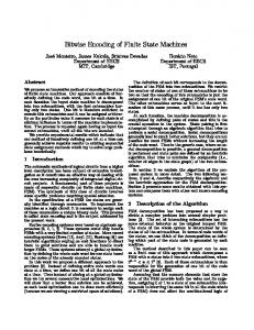
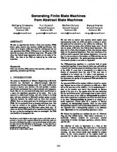
1.1. Need for New Techniques of State Assignment Existing automatic state assignment techniques targeting optimal PLA implementations of combinational logic are inadequate for producing optimal multilevel implementations. This is illustrated in Figs. 1-3. Using a state assignment program targeted toward PLA implementations the states of the FSM in Fig. l are given the codes in Fig. 2(a). This encoding produces a six product term PLA (Fig. 2(b)) after two-level minimization. After multilevel logic optimization, the resulting network contains 16 gates and is shown in Fig. 2(c). A different assignment of codes (Fig. 3(a)) produces a larger PLA with seven product terms (Fig. 3(b)), but a smaller multilevel logic network with 15 gates (Fig. 3(c)). This example illustrates the need for state assignment techniques targeted toward a different object, namely, optimal multilevel implementations of FSM combinational logic.

1.2. State Assignment for Multilevel Logic Implementations In the sequel, we present a strategy for finding a state assignment of a FSM which minimizes an estimate of the area used by a multilevel implementation of the combinational logic. The estimate considered here is consistent with the estimate used by multi-level logic optimization algorithms [lo]-[ 121: the number of literals in a factored form for the logic. We have developed algorithms which produce a state assignment that heuristically minimizes the number of literals in the resulting combinational logic network afrer multilevel logic optimization. Multilevel logic optimization programs like MIS [ 113 and SOCRATES [ 121 primarily use algebraic techniques for factorizing and decomposing the Boolean equations by identifying common sub-expressions. Our heuristics are based on maximizing the number and size of common subexpressions that exist in the Boolean equations that de-

0278-0070/88/1200-1290$01.OO

0 1988 IEEE

1291

D E V A D A S et al.: M U S T A N G : FINITE S T A T E M A C H I N E S

-0 st0 sto 0 11 sto sto 0

01 sto 0- stl 11 SI1 IO stl 1- st2

00 st2 01 st2 0- st3 1 1 st3

We have obtained results over a wide range of benchmarks which illustrate the efficacy of our techniques. Literal counts averaging 20-40 percent less than the state assignment program KISS [5] and random assignment techniques have been obtained. Preliminaries and definitions are given in Section 11. In Section 111, the basic approach followed to obtain a good state assignment is described. In Section IV, two algorithms are presented. The embedding algorithm used is presented in Section V. Results on the benchmark examples are presented in Section VI.

stl stl 1 slo 0 st2 1 st2 1 stl 1 st3 1 st3 1 st2 1

Fig. 1. Example FSM. stO -> 00 sl?. -> 1 1

-> 01 s13 -> 10

SI1

(a) 10-1 1 1 10- 10 01 0-0 -1

- 1 1-

100 01 0 10 1 01 1 01 1 10 1

(b)

Inputs

output

&

Present

Next

States

States

11. PRELIMINARIES 2.1. Basic Definitions A variable is a symbol representing a single coordinate of the Boolean space (e.g., a ) . A literal is a variable or its negation (e.g., a or a ) . A cube is a set C of literals such that x E C implies X C (e.g., { a , b , C } is a cube, and { a , a } is not a cube). A cube represents the conjunction of its literals. The trivial cubes, written 0 and 1, represent the Boolean functions 0 and 1, respectively. An expression is a set f of cubes. For example, { { a }, { b , c } } is an expression consisting of the two cubes { a } and { b, C}. An expression represents the disjunction of its cubes.

2.2. Representations of FSM’s An FSM is represented by two equivalent structures. Fig. 2 . (a) State assignment. (b) Minimized PLA implementation. (c) Optimized multilevel implementation. sto -> 00 st2 -> 01

stl -> 10 S I 3 -> 1 1

(a) 10 10 0- 11 01 -1-01 0- 1-1 -1 0- -1

01 1 01 0 100 01 1 10 1 01 1 10 1

~::(b)

Inputs Present States Bc

(1) It is State Transition Graph G( V , E , W (E ) ) where V is the set of vertices coresponding to the set of states S , were 1) S )I = Ns is the cardinality of the set of states of the FSM, an edge ( v i ,2;. ) joins U , to vj if there is a primary input that causes the FSM to evolve from state U ; to state vj, and W ( E ) is a set of labels attached to each edge, each label carrying the information of the value of the input that caused that transition and the values of the primary outputs corresponding to that transition. (2) It is a State Transition Table T ( I , S , 0 ) where I is the set of inputs, S is the set of states as above, and 0 is the set of outputs. We assume that the primary inputs and outputs of the FSM are in Boolean form. A row of the table corresponds to an edge in the state-transition graph. The table has as many rows as edges of state graph and as many columns as

output

zNext

States

(c)

Fig. 3. (a) State assignment. (b) Minimized PLA implementation. (c) Optimized multilevel implementation.

scribe the combinational logic part of the FSM after the states have been encoded but before logic optimization. The state assignment algorithms find pairs or clusters of states which, if kept minimally distant in the Boolean space representing the encoding, result in a large number of common sub-expressions in the Boolean network.

Nj

+ No + 2

where Niis the number of bits used to encode the inputs, No is the number of bits used to encode the outputs, and 2 refers to the present state and the next state. The matrix has Boolean entries for the inputs and outputs and “symbolic” entries for the columns corresponding to the present and next states, carrying the name of the present state and of the next state, respectively. The rows of the matrix are divided into two fields: the first field contains the input pattern and the names of the present state, the second field contains the output pattern and the names of

1292

IEEE TRANSACTIONS ON COMPUTER-AIDED DESIGN. VOL 7. NO. 12. DECEMBER 1988

the next state. Note that the input pattern may contain don’t care entries.

2.3. State Assignment for Multilevel Logic The state assignment problem consists of assigning a string of bits (code) to each of the states, so that no two states have the same code. After a code has been assigned, the FSM can be implemented trivially once the storage elements (flip-flops) have been chosen, with a PLA. For example, assume that the storage elements are D flip-flops (one per bit). Then, each edge ( v i ,uj ) of the state transition graph or row of the state transition table, corresponds to a product term, with the input part represented by the bits specified in the label w( ( ui,uj ) ) for the primary input and the bits forming the code for v i(the present state), and the output part represented by the bits forming the code for uj and the bits specified in w ( ( vi, vj)) for the primary outputs. This representation of the FSM can be optimized using a two-level logic minimizer as ESPRESSO [ 131 to reduce the number of product terms needed to implement the logic function. Of course, different encoding of the states yield different logic functions. It is of great interest to assign codes to states so that the final optimized PLA has a few product terms as possible. Algorithms have been proposed that solve this problem by using a symbolic optimization step to determine a set of constraints on the encoding to guarantee that certain product terms could be eliminated in the final implementation [ 5 ] , [7]. However, in some cases, the size of the PLA remains too large to satisfy timing or area constraints. In this case, a multilevel implementation of the logic is in order. The two-level logic description is then mapped into a multilevel implementation by factoring and decomposing the logic functions corresponding to the outputs. According to the particular target technology, e.g., CMOS standard cells, CMOS static gates laid out in the gate-matrix style or Weinberger arrays, a decomposition and factorization will be more effective than others. Algorithms have been proposed that perform this step effectively (e.g., [lo]-[ 121). These algorithms represent the logic to implement as a Boolean network, i.e., a directed graph where each node corresponds to a logic function with one output and an arc is provided between two nodes if the output of one function is an input of the other. Because the output of each node is unique, a node and an output are in one-to-one correspondence. In principle, in these algorithms, a cost function that is different according to the final implementation should be used. However, due to the many different technologies used, it is very difficult to identify a meaningful cost function that could be optimized effectively. Thus an estimate for the final area is used. An estimate that has been used successfully is the number of literals in a factored form of the logic function. Then, the optimal state-assignment problem can be formulated as the problem of assigning codes to the states so that the total number of literals in the factored form of the logic finction is minimized. It is certainly difficult to devise a measure of how many

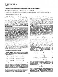
literals a particular state assignment will yield after multilevel logic optimization has been carried out, because of the great complexity of the algorithms used for this purpose [ l l]. 111. THE BASICIDEA 3.1. Operations in Multilevel Logic Optimization The key point in the proposed algorithms for the state assignment problem is the model used to predict the results obtained by the multilevel logic optimizer after the encoding has been performed. We focused on the operations of MIS [ 1 13, the Berkeley logic optimizer. The algorithms in MIS [ l l ] can be classified in two categories: algebraic and Boolean methods. It is very difficult to model the optimization achieved by MIS with the use of Boolean methods, while it is feasible to predict at least some of the operations that the algebraic division algorithms use to minimize the logic. Among the several algebraic optimization algorithms used by MIS are factoring of logic equations, common sub-expression identification and common cube extraction. These three techniques are illustrated in Fig. 4. The latter two techniques are algebraic division techniques, expressions are divided by common cubes or sub-expressions in order to produce smaller expressions with new intermediate variables. Common cube extraction is actually a subset of common sub-expression identificationa sub-expression may be a single cube. As illustrated in Fig. 4, extracting common cubes results in a network with fewer literals than the original network. The algorithm presented in this paper tries to maximize the number of common cubes that can be found by the logic optimization algorithms in the encoded two-level network. Maximizing the number of common cubes results in a large number of good factors that can be extracted during optimization to produce a reduced literal multi-level representation.

3.2. Influence of Encoding on the Number of Common Cubes There are two basic processes behind the influence of state assignment on the number of common cubes in the encoded state transition table (a two-level representation) which is the starting point for multilevel logic optimization. We now analyze these two processes. We focus on the second field (the present state field) in the STT of the machine shown in Fig. 1. If we assigned the states stO and st2 with codes of distance Nd, then the lines of the next state stl will have a common cube with Nb - Nd literals (due to edges 3 and 8 in the STT). Similar relationships exist between other sets of states. We shift focus to the third field (the next state field) of the STT. If we assign the states stO and s t 2 with codes of distance N d , then the present state st 1 becomes a common cube for Nb - Nd next state lines whatever its code is (due to edges 5 and 6 in the STT). The number of literals in the common cube is, of course, N h . Again, similar relationships exist between other sets of states in the machine.

DEVADAS et u l . : MUSTANG: FINITE STATE MACHINES

Factoring:

ace

+ bce + de ->

((a

+ b) c + d ) e

Common sub-expression identification: ace + bce + de -> sce + de ade + M e + af -> sde + af s=a+b

Common cube identification:

ace + bcef + de -> tc + uc ade + bdef + af -> td + ud t = k f u=ae

+ de + af

Fig. 4. Factoring, common sub-expression and common cube identification.

The input and output spaces (the first and fourth fields) also have an influence on the number of common curves after encoding. If two different input combinations, i , and i2, produce the same next state from different or same present states, then we have a common cube corresponding to i , n i2 in the input space. Similarly, outputs asserted by different present states have common cubes corresponding to their intersections. Given a machine, we have thus a large set of relationships between state encoding and the number/size of common cubes in the network prior to logic optimization. We can estimate the reduction in literal count or the “gains” that can be obtained by coding a given pair of states with close codes so single/multiple occurrences of common cubes can be extracted. Given these gains for each pair of states, we can attempt to find an encoding which maximizes the overall gain. There arises a complication in gain estimation. Firstly, while the number of literals in the common cubes can be found exactly, the number of occurrences of these cubes depends on the encoding of the next states. In our example, assume that s t l was assigned 111 and st3 was assigned 110. We have a common cube 11 (with 2 literals) for the next state lines but the number of occurrences of the this common cube depends on the number of 1’s in the code of st2 (which we do not know). This problem is alleviated by treating the gains as relative merits rather than absolute and using an average-case analysis (Section 4.1.2). It should be noted that these statically computed gains interact. Extracting some common cubes can increase the level (to the outputs) of other common cubes and can also decrease the gain in extracting them. For instance, a sequence of two cube extractions on a two-level network can produce a three- or a four-level network. Statically computing gains and maximizing the number of common cubes works because, given a particular encoding, the optimal sequence of cube extractions to produce a minimal literal multi-level network can be found by the logic optimizer. Our goal then is to find an encoding that maximizes the number of common cubes in the initial twolevel network.

3.3 The Global Strategy Our approach is to build a graph G M (V , E,,,, W ( E,,, ) ) where V is in one-to-one correspondence with the states

1293

of the finite state machine, EM is a complete set of edges, i.e., every node is connected to every other node, and W ( E,,, ) represents the gains that can be achieved by coding the states joined by the corresponding arc as close as possible. These gains are statically and independently computed by enumerating the direct relationships between the input, state, and output spaces. Then, the states are encoded, using this graph to provide the cost of an assignment of a state to a vertex of the Boolean hypercube. A critical part of our approach is the generation of W ( E,,, ). We have experimented with two algorithms: one assigns the weights to the edges by taking into consideration the second and fourth fields of the state transition table, and is henceforth called fanout-oriented. The second algorithm assigns weights to the edges by taking into consideration the first and third fields and is henceforth called fanin-oriented. The fanout-oriented algorithm attempts to maximize the size of the most frequently occurring common cubes in the encoded machine prior to optimization. The fanin-oriented algorithm attempts to maximize the number of occurrences of the largest common cubes in the encoded machine prior to optimization. These two algorithms are based on the two different processes behind the influence of state assignment on the number of common cubes in the network described earlier.

IV. ALGORITHMS FOR GRAPHCONSTRUCTION In this section, we present a fanout-oriented and a faninoriented algorithm which define a set of weights for the undirected graph GM(I/, E , W ( E,,, )). The weights represent a set of closeness criteria for the states in the machine which reflect on the number of common cubes in the encoded machine prior to optimization. Both these algorithms have a time- and space-complexity polynomial in the number of inputs, outputs and states in the machine to be encoded. In the sequel, the two algorithms are described and analyzed. 4.1. A Fanout-Oriented Algorithm This algorithm works on the output and the fanout of each state. Present states which hssert similar outputs and produce similar sets of next states are given high edge weights (and eventually close codes) so as to maximize the size of common cubes in the output and next state lines. 4. I . I . Algorithm Description: The algorithm proceeds as follows: Construct a complete graph G M (I/, E,,,, W ( EM)), with the edge weight set empty. For each output, all the labels, W (E,,, ), in the state-transition graph G , are scanned to identify the nodes which assert that output. No sets of weighted nodes which assert each output are constructed. If a node asserts the same output more than once it has a correspondingly larger weight in the set. For each next state, sets of present states producing that next state are found ( N , sets are constructed).

IEEE T R A N S A C T I O N S ON C O M P U T E R - A I D E D D E S I G N , VOL. 7, NO. 12. DECEMBER 1988

1294

The pseudocode below illustrates these steps of the procedure. nw stores the weight of the nodes in each of the different sets.

for(i= l ; i 5 N o ; i = i + 1 ) { foreach( edges e(uk, U / ) E G ) { i f ( W(e).output[i]is 1 ) { OUTPUT-SETi = OUTPUT-SET U Uk nw(OUTPUT-SETi, uk) = nw(0UTPUT-SET,, uk) + 1

1

3

1

foreach( edges e ( v k , U / ) E G ) { N-STATE-SET/ = N-STATE-SET, U Uk nw(N-STATE-SET[, uk) = nw(N-STATE-SET,, uk) + 1

1 ( 3 ) Using these No OUTPUT-SET AND N, NSTATE-SET sets of nodes, W ( EM) is constructed. The edge weight, we, is equal to the multiplication of the weights of the two nodes corresponding to it across all the sets. The weights corresponding to the next state sets have a multiplicative factor equal to the half the number of encoding bits, N b / 2 . The reasoning behind the use of a multiplicative factor is given at the end of the section. The pseudocode for the calculation of we is shown below.

4.1.2. Analysis: We now analyze the fanout-oriented algorithm. The first step of the algorithm entails enumerating the relationships between the present states and the output space. If two different present states assert an output, it is possible to extract a common cube corresponding to the intersection of the two state codes. By constructing the No different output sets and counting the number of times a pair of states occurs together in each output set, the algorithm effectively computes the number of occurrences of the common cube X fl Y , for all states X and Y. We have to take into account the fact that a state may assert the same output for many input combinations-this corresponds to the weight nw ( ). For two states that assert the same out-

put a multiple number of times, each pair of edges will have the common cube. Accordingly, the weights n w ( ) are multiplied. In the second step, the next states produced by each pair of present states are compared. A state pair which produces the same next state has an associated common cube corresponding to the pairwise intersection. The number of occurrences of this common cube is dependent on the number of 1's in the code of the next state and therefore cannot be estimated exactly (unlike in the first step). We assume that the average number of 1's in a state's code is N b / 2 . Since we are concerned with relative rather than absolute merits, the approximation that each common cube occurs in N b / 2 next state lines is a good one. Thus we have a multiplying factor of N b / 2 in the second step. Ideally, this factor should be a function of the encoding and not a constant for all state pairs. Given the number of occurrences of different common cubes in the machine, this algorithm assigns weights so as to maximize the size of the most frequently occurring cubes.

4.1.3. An Example: The graph generated by the fanout-oriented algorithm for the example FSM of Fig. 1 is shown in Fig. 5. The output set corresponding to the single output is ( s t 0 2 ,stl 3 , s t 3 * ) . The next state sets are stO + ( s t 0 2 , s t l I ) , stl ( s t O ' , s t l ' , s t 2 ' ) , s t 2 + ( s t l ' , s t 2 ' , s t 3 ' ) and st3 + ( s t 2 ' , s t 3 ' ) . The superscripts denote the weights n w ( ) for each state in each set. The weight of the edge between 1 X 1) the states s t 2 and st3 with Nb = 2 is ( 1 X 1 X N b / 2 + 3 X 2 = 8 . Similarly, the other edge weights can be calculated. +

+

4.2. A Fanin-Oriented Algorithm The algorithm described above ignored the input space. The algorithm works well for FSM's with a large number of outputs and small number of inputs. However, the number of input and output variables could both be quite large. In this section, we describe a fanin-oriented algorithm which operates on the input and fanin for each state. Next states which are produced by similar inputs and similar sets of present states are given high edge weights (and eventually close codes) so as to maximize the number of common cubes in the next state lines. 4 . 2 . 1 . Algorithm Description: The algorithm proceeds as follows: ( 1 ) The graph GMis constructed. N, sets of weighted next states which fan out from each present state in G are constructed as shown below. nw stores the weight of each node in all the sets. foreach( edge e ( v k , U / ) E G ) { P-STATE-SET, = P-STATE-SET, U U / nw(P-STA TE-SET,, ) = nw(P-STATE-SETk, v l) + 1

1

D E V A D A S et al.: M U S T A N G : FINITE S T A T E M A C H I N E S

1295

1

* S

u Fig. 5 . Graph generated by fanout-oriented algorithm.

( 2 ) For each input, sets of next states are identified which are produced when the input is 1 and when the input is 0. 2 X Ni such sets are constructed as shown below.

for(i=l;i + 11 i f ( W ( e ) . i n p u t [ i ]is 0 ) { INPUT-SETO~~~ = INPUT-SETO~~, U nw(INPUT-SET°FFi, U , ) = nw(INPUTS E T O ~ ~ ,U , /) 1 INPUT-SETO~,

I

I

I

+

( 3 ) The weights on the edges in the graph, we, are found using the Ni INPUT-SEToN, N, INPUTSEToFFand N, P-STATE-SET sets of nodes as illustrated in the pseudo-code below. Between each pair of nodes in GM,an edge with weight equal to the multiplication of the weights of the two nodes across all the present state sets (scaled by Nb) and all the input sets is added

t

T

5

L

st3

u

Fig. 6. Graph generated by fanin-oriented algorithm.

ing the number of times a pair of states occurs together in each input set, the algorithm computes similarity relationships between all next state pairs in terms of the inputs. Giving next state pairs that are produced by similar inputs high edge weights will result in maximizing the number of occurrences of the largest common input cubes in the next state lines. In the second step, the present states producing each pair of next states are compared. If two different next states are produced by the same present state. the state is common to some next state lines. The number of occurrences of this common cube is deperldent on the intersection of the two next state codes. To maximize the number of occurrences of these cubes, next state pairs which have many common present states are given correspondingly high edge weights. Since each of these cubes have Nb literals (as opposed to a single literal for a single input), we have a multiplying factor of Nb while combining the weights computed in the two steps. Given the sizes of the different common cubes in the machine, this algorithm assigns weights so as to maximize the number of occurrences of these cubes. 4 . 2 . 3 . An Example The graph generated by the fanin-oriented algorithm for the example FSM of Fig. 1 is shown in Fig. 6. As can be seen, the weights of the edges in the graph are different from those generated by the fanout-oriented algorithm (Fig. 5 ) . Herewehavetheinputsetsil(0) ( ~ t l ~ , s t 3 ~ ) , i l ( l ) ( ~ t O ~ , s t 2i 2~( )0 ,) (stO',stl',st2')andi2(1) ( stO 2 , st 1 I , st 2 I , sc 3 ) . The present state sets are stO -, ( s t o 2 , s t l '1, stl ( s t o ' , s t l I , s t 2 ' ) , st2 ( s r l I , s t 2 l , s t 3 l ) and st3 ( s t 2 l ) . The weight of the edge 2 X 1) between stO and stl for Nb = 2 is ( 1 X 1 Nb X ( 2 X 1 1 X 1 ) = 9. The other edge weights are calculated in a singular fashion. +

+

+

+

-+

+

+

+

+

+

V . THE EMBEDDING ALGORITHM

4 . 2 . 2 . Analysis: We now analyze the fanout algorithm. The first step of the algorithm entails enumerating the relationships between the input and next state space. A next state produced by two different input combinations i, and i2 has a common cube il fli 2 . The size of this cube can be found. By constructing the 2 X Ni different input sets and count-

The algorithms presented above generate a graph and a set of weights, like the graphs of Figs. 5 and 6, to guide the state encoding process. The problem now is to assign the actual codes to states according to the analysis performed by the fanin and the fanout-oriented algorithms. This problem is a classical combinatorial optimization problem called graph embedding. Here GM has to be embedded in the Boolean hypercube so that the adjacency relations identified by GM are satisfied in an optimal way. Unfortunately, this problem is NP-complete and there is little hope to solve it exactly in an efficient way. Several heuristic approaches have been taken to solve variations of this problem (e.g., [14], [81, [151). In 1141

IEEE T R A N S A C T I O N S O N C O M P U T E R - A I D E D DESIGN, VOL. I . NO. 12. DECEMBER 1988

1296

and [ 151 distance relations are required to be satisfied during graph embedding. Of course, it may not be possible to satisfy all of them and some constraints (which are heuristically picked) may be relaxed. Similarly in [8], where clusters of states are recognized as in the faninl fanout-oriented algorithms, join and fork rules are specified which if satisfied result in the merging of product terms. Our problem is different in sense that the goal is to minimize a cost function rather than attempting to satisfy distance relations. We use a heuristic approach to this embedding problem that has given satisfactory results. The heuristic algorithm is called wedge clustering. This algorithm is used to assign codes to the nodes in GM to minimize Ns

We can prove the following optimality result about the embedding heuristic. For convenience in notation, we assume that we ( y i , y i ) = 0 V i 3 yi E GM. , Theorem 1: At a given iteration, if the Nb states y ~y2, . . . ,yNbare given unidistant codes from the selected state v l and if we ( e M ( v lY,; ) ) 2 we ( e M ( y i , Y j ) ) + we ( e M ( ~ iY, , ) ) , 1 Ii , j ; k IN b ; i f j # k

(1)

then the assignment is optimum for this cluster of Nb states, i.e.,

+1

Ns

C C i=l j=i+l

we ( e M ( v i ,v i ) ) * dist (enc ( v i ) ,enc ( v j ) )

where the vk are the vertices in G,, we ( e M ( vk, vl ) ) is the weight of the edge, e , between vertices vk and U [ , enc ( v k ) is the encoding of vertex vk. The function dist ( ) returns the distance between two bindary codes. The graphs generated by the fanout- and fanin-oriented algorithms have a certain structure associated with them, especially for large machines. In these graphs, typically small groups of states exist that are strongly connected internally (edges between states in the same group have high weights) but weakly connected externally (edges between states not in the same cluster have low weights). The embedding heuristic has been tailored to meet the requirements of our particular problem. The heuristic exploits the nature of the graph by attempting to identify strongly connected clusters and assigning states within each cluster with uni-distant codes. The embedding algorithm proceeds as follows. Clusters of nodes with the cardinality of the cluster no greater than Nb 1 and consisting of edges of maximum total weight are identified in G,. Given G,, the identification of these clusters is as follows-a node, v1 E G M ,with the maximum sum of weights of any Nb connected edges is identified. The Nb nodes, y l , y 2 , . * , yNbwhich correspond to the Nb edges from vl and v I are assigned minimally distant codes from the unassigned codes ( v l may have been assigned already, so may the other yi ). A maximum of Nb nodes are chosen so the yi can be (possibly) assigned unidistant codes from v l . After the assignment, v l and all the edges connected to vl are deleted from GM and the node section/code assignment process is repeated till all the nodes are assigned codes. The pseudocode below illustrates the procedure.

+

GG = GM while ( GG is not empty) { E

GG so

we ( e M ( u ly, i ) ) * dist (enc Nb

i= I

we ( e , ( v , , y i )) is

maximum assign the yi and v I minimally distant codes from unassigned codes

(VI),

enc ( Y i ) )

Nb

* dist (enc ( v i ) ,enc ( y j ) ) is minimum. Proof: We have to prove that no assignment of codes to states can produce a cost which is less than the cost, C ( v1), produced by assigning the Nb states with uni-distant codes from vl. We have

Nb

Nb

-

since the y l , * ,yNbhave uni-distant codes from v 1 and, therefore, are distance-2 from each other. To decrease the cost, the distances between the codes of the yi have to be reduced from 2 to 1. This can only be done at the expense of an increase in the distance between some of the yi and vl from 1 to 2. There are three possible ways of doing so. First, we can select any state y s from y l , * * Y N b and code the rest of the yi and v I with unidistant codes from ys. Without loss of generality, assume we select y l . We know, since we selected v1 initially, that 9

Nb

Using (2) above, it can easily be shown that Nh

Nh

Nb

Select v1 E G G , y i

Nh

C i=l

Nh

+ 2 * i C= 2 C

j=i+l

and similarly, for C ( y 2 ) ,

*

we ( e M ( y i y, j > >

, C(YN*).

1297

D E V A D A S er al.: M U S T A N G : FINITE S T A T E M A C H I N E S

The second alternative in assigning codes is to select a ys and assign it a code which is unidistant from two other yi (Only two yi can be chosen since the yi are distance-2 from each other). This code will be distance-3 from the unselected yi and will be distance-2 from u l . Without loss of generality, assume that y I was selected and assigned a unidistant code from y2 and y 3 . We have

Expanding C ( vl ), we have C(Vl> =

we ( e M ( %

YI

Nh

3

Nh

c ( Y =~ ),Z we (eM(u1, ~ i > + ) we ( ~ M ( Y Y, ,i > ) =2 i=2 I

+ 2 * we (4% Y l ) ) + 2 * we ( Nb

4 Y 2 ,

3

We(eM(yi,

Yj))

Nb

+ 2 * iC C w e ( e M ( ~ iY, j ) ) =2 j=i+ 1 Nb

+ 3 * iC we (eM(y1, Y i ) ) . =4 Expanding C ( u1), we have 3

Nb

,zwe +

we

( e M ( ~ ’ 1 ,Y i > ) +

(eM(V1, Y l ) ) Nb

+2*

2

*

.zwe

I

=2

+ 2 * we

( ~ M ( Y , ,Y i > )

(eM(Y2,

n>>

we

+ we we

1

(eM(Yi, Y j ) )

we

(eM(Y1, Yi)).

Canceling terms from C ( y I ) and using relation (l), shows that C ( y l ) 2 C(v,). The third alternative in assigning codes is to select a state y s and 2 < p < N6 - 1 states from the remaining yi and make these p states uni-distant from ys. y s will be uni-distant from u l , and p states will be distance-2 from ul and will be distance-2 from each other. I f p I2 then we are back to the second alternative (or worse) which is nonoptimal. Similarly, p = Nb - 1 brings us back to the first alternative which is nonoptimal. Assuming y 1 and y 2 , . . . , yP + are selected, we have P+ I

C ( Y 1 ) = we

( C M ( h Nh

(%(Yi,

Yd)>

Nb

i=2 j=i+l

i=4

* we ( e M ( y i , Y j ) )

( e M ( ~ i Y, j ) )

Nb

+2*

Canceling terms from C ( y 1) and using relation (l), shows that C ( y l ) 2 C ( v l ) . In the general case, more than one ys, each with an associated set of states from the remaining y i , may be selected and each set made unidistant from ys. The proof for this case is more involved but follows in a similar way as for the previous case, expanding C ( ul ) and using relation (1). Q.E.D. Thus we have a heuristic which is optimal for a graph satisfying relation (1) at each iteration of the embedding if sets of minimally distant codes can be found. It produces good (though perhaps sub-optimal) solutions for graphs satisfying we (eM(uI, Y i ) ) 2 RAT

Nb

+ 2 * i = 4 j =C i+l 3

Nh

Nb

+ 2 * i=4 j=i+l

c(~l => 1-2

Nb

Y3))

Y1)) + 2

*

.zwe ( e M ( %

I

=2

Yi))

Ii , j ;

k

INb; i #

j # k

where RAT is close to 1. This, coupled with the fact that typical graphs produced by the fanout- and fanin-oriented algorithms have strongly connected clusters of states, makes the embedding algorithm eminently suitable for our purpose. The algorithm is quite fast and has a worst case time complexity of O(Ni(1og ( N s ) N b ) ) . Initially, the N s - 1 fanout edges from each of the N s states are sorted in decreasing order of weights which takes O ( N i log ( N s ) ) time. The embedding itself may require a maximum of N , - N6 iterations. This is because in the first iteration, Nb 1 states are encoded and in the worst case only one state is encoded in following iterations. To select a state with maximum weight of any Nb connected edges can be accomplished in o ( N s N b ) time, giving an overall time complexity of o ( N ; ( log ( N~ + N~ ) 1. The embedding algorithm is illustrated in Fig. 7 using a small example with 5 states, to be encoded using 3 bits. Initially, the node corresponding to state st 3 is selectedit is the node with the maximum set of any 3 edge weights. The states corresponding to these three edges are stO, st 1 and st2. The three states are given codes uni-distant from st3. st3 and its edges are deleted from the graph. The selection process continues, picking st 1 from the modified graph and encoding st4. This completes the encoding.

+

+

1298

IEEE TRANSACTIONS O N COMPUTER-AIDED DESIGN. VOL. 7. NO. 12. D E C E M B E R 1988

N,

-

= 3 STATISTICS OF

TABLE I BENCHMARK EXAMPLES

s t 3 (stO, s t l , s t 2 ) u(AMpLE

st4

ologc& 001

sto

st2

100

st3 stl

000 s t o 010 s t 2

4

+

4

--t

001 100

thnp

lese

-

'

s t l ( S t O , st2, s t 4 ) st4

1

2 7

7 , 8

19

1 0 , 4 ! 16 1 4 2 6 1 3 7 1 6 1 4 , 5 , 4 1 2 3 I 27 5

3

dkl5x dklbx

Itenc

#states

%but

4 7 2 7

bbara bbsse 'bbtas

2

110 hon9

Fig. 7 . An embedding example.

VI. RESULTS We have run 20 benchmark examples (which have b e m obtained from various university and industrial sources) representing a wide range of finite automata on different state assignment programs as well as on our two algorithms. The size statistics of the examples are given in Table I, with the minimum possible encoding for each FSM indicated under the column #enc. The results obtained via random state assignment (RANDOM-A and RANDOM-B), using the state assignment program KISS (KISS), the fanout-oriented algorithm (MUST-P) and the fanin-oriented algorithm (MUST-N) for multi-level implementations are summarized in Tables I1 and 111. The number of literals after running through two optimization scripts in the multi-level logic synthesis tool MIS [ 111 are given for each of the state assignment techniques. The literal counts of Table I1 were obtained using a short optimization script and those of Table 111 using a much longer optimization script (which produces better results). The literal counts under RANDOM-A were obtained using a statistical average of 5 different random state assignments (using different starting seeds) on each example. RANDOM-B was the best result obtained in the different runs. RANDOM-B is significantly better than RANDOM-A especially for the smaller examples. MUSTANG is the best result produced by either the fanout or the fanin-oriented algorithm for each given example. MUSTANG can be constrained to use any number of encoding bits greater than or equal to the minimum. For all examples MUSTANG was run using the minimum possible bit encoding. Minimum bit encoding has been found to be uniformly good for multi-level logic implementations. KISS typically uses a 1-3 bits more than the minimum encoding length. The time required by MUSTANG for encoding these benchmarks varied between 0.1 CPU seconds for the small examples to 100 CPU seconds for the largest example, scf, on a VAX 11/8650. The algorithms developed have achieved the goal of producing encodings which produce minimal area implementations after multilevel logic optimization as illustrated in Tables I1 and 111. The literal counts obtained by MUSTANG are on the average 30 percent better than random state assignment and 20 percent better than KISS. In some cases, the fanout-oriented algorithm does better than the fanin-oriented algorithm, when ignoring the common

~

planet

I

51

1 8 sla __.__--

!

1

la"

1

4

2

0

20 128 8 4

56 4

!

48

~

6

6

1

6 ,

5

1

5

7 ' 3 , 2 1

TABLE I1 RESULTSOBTAINED USING SIMPLE CHART RANDOM-A

1

20 61

hon

Lon9

j

'

111 305

'

18 52

100 260

116 185

21

37

1

!

18

22

25

U)

18 20

TABLE 111 RESULTSOBTAINED USING INTENSIVE SCRIPT

TOTAL

1

4.594

139

I 4210 1

137

I

3754

1

1.14

1

I

I

49 3296

1299

DEVADAS et al.: MUSTANG: FINITE STATE MACHINES

KISS

RANDOM-B #hl #gate cse

dk16x ~~

keyb

planu sl sla scf

240 394 j 311 654 354 337 922 342

1

1 tbk.min I

MUSTANG-N #hl #Rae .

#E-

#iil

203 95 315 143 158 1 213 1 112 547 290 249 352 I73 174 131 258 169 861 401 445 170 381 j 169 115

175

,

I 1

I 1

I

I

I 1

1 1 1

220 290 210 563 160 141 852 297

105

1 1

I

124 112 267 93 83 393 130

1

sub-expressions in the input space is a good approximation. MUSTANG does comparatively better than random assignment or KISS in the shorter optimization script case than in the more complex optimization script. This is to be expected since MUSTANG models only the common cube extraction process in multilevel logic optimization. In the short optimization script, cube factors dominate in the reduction of the size of the network. More complicated factors, not modeled by MUSTANG, come into play in the complex optimization script. For any given example, the literal counts obtained using MUSTANG and short or long optimization scripts are comparatively closer than using KISS or random assignment. For example, in bbara, using random assignment produces 120 literals after quick optimization versus 76 after a long optimization (on an average). The corresponding number for MUST-P are 81 and 68, respectively. MUSTANG eases the job of the multi-level logic optimizer, by providing a larger number of easily detectable factors in the network before optimization-a short script can produce good results. Also, the time taken by MIS to optimize MUSTANG encoded examples is significantly shorter (20-40 percent) than to optimize examples encoded using different techniques. Again, this is because a large number of easily detectable factors exist in the preoptimized network. Both MUSTANG and MIS optimize for literal counts rather than the number of gates in the network. MIS may produce arbitrarily complex gates in an optimized network. In many cases, these gates have to be mapped to a specific technology library. It is worthwhile to see if the gains in literal counts do produce networks with fewer gates. The number of gates in the benchmark examples after intensive logic optimization and technology mapping are given in Table IV for the different state assignment techniques. Only the largest examples are shown, the small examples had insignificant numbers of complex gates. VII. CONCLUSIONS All previous work in automatic state assignment has been targeted toward two-level logic implementations of finite state machines. Multilevel logic implementations can be substantially faster and/or smaller than corresponding two-level implementations. We have shown the need for new techniques for state assignment directly tar-

geting multi-level logic implementations and developed algorithms for this purpose. As compared to existing techniques, significant reductions in literal counts, averaging 20-40 percent have been obtained on benchmark examples. Further work includes attempting to merge the fanin and fanout-oriented approaches and predicting more complicated multilevel logic optimizations like common kernel extraction and Boolean factoring.

REFERENCES [I] D. B. Armstrong, “A programmed algorithm for assigning internal codes to sequential machines,” IRE Trans. Electron. Comput., vol. EC-11, pp. 466-472, Aug. 1962. [2] T. A. Dolotta and E. J. McCluskey, “The coding of internal states of Sequential machines,” IEEE Trans. Electron. Comput., vol. EC13, pp. 549-562, Oct. 1964. H. C. Torng, “An Algorithm for finding secondary assignments of synchronous sequential circuits,” IEEE Trans. Computers, vol. (2-17, pp. 416-469, May 1968. G. D. Micheli, A. Sangiovanni-Vincentelli,and T . Villa, “Computer-aided synthesis of PLA-based finite state machines,” in Proc. Inr. Con$ on Computer-Aided Design, Santa Clara, CA, November 1983, 154-156. G. D. Micheli, R. K. Brayton, and A. Sangiovanni-Vincentelli, “Optimal state assignment of finite state machines,” IEEE Trans. Computer-Aided Design, vol. CAD-4, pp. 269-285, July 1985. A. J. Coppola, “An implementation of a state assignment heuristic,’’ in Proc. 23rd Design Automation Conf., Las Vegas, NV, July 1986. G. D. Micheli, “Symbolic design of combinational and sequential logic circuts implemented by two-level macros,’’ IEEE Trans. Computer-Aided Design, vol. CAD-5, pp. 597-616, Oct. 1986. G. Saucier, M. C. Depaulet, and P. Sicard, “ASYL: A rule-based system for controller synthesis,” IEEE Trans. Computer-Aided Design, vol. CAD-6, pp. 1088-1098, Nov. 1987. C. Tseng et a l . , “A versatile finite state machine synthesizer,” in Proc. Int. Con5 on Computer-Aided Design, Santa Clara, CA, pp. 206-209, Nov. 1986. R. K. Brayton and C. T. McMullen, “Synthesis and optimization of multistage logic,” Proc. ICCD, Oct. 1984. R. K. Brayton, R. Rudell, A. Sangiovanni-Vincentelli, and A. Wang, “MIS: A multiple level logic optimization system,” IEEE Trans. Compurer-Aided Design, vol. CAD-6, pp. 000-0000, Nov. 1987. K. Bartlett, G. D. Hachtel, A. J. D. Geus, and W. Cohen, “Synthesis and optimization of multi-level logic under timing constraints,” in Proc. Inr. Conf. on Computer-Aided Design, Santa Clara, CA, pp. 290-292. Nov. 1985. [13] R. K. Brayton, C . T . McMullen, G. D. Hachtel, and A. L. Sangiovanni-Vincentelli, Logic Minimization Algorithms for VLSI Synthesis. New York: Kluwer Academic, 1984. [I41 G. D. Micheli and A. Sangiovanni-Vincentelli, “Multiple constrained folding of programmable logic arrays: Theory and applications,” IEEE Trans. Computer-Aided Design, vol. CAD-2, July 1983. [I51 R. L. Graham and H. 0. Pollak, “On embedding graphs in squashed cubes,” in Graph Theory and Applications 303. New York: Springer Verlag, 1972.

* Srinivas Devadas received the B.S. in electrical engineering from the Indian Institute of Technology, Madras, India, in 1985, the M.S.E.E. and Ph.D. degree from the University of California, Berkeley in 1986 and 1988, respectively. He is currently an Assistant Professor of Electrical Engineering and Computer Science at the Massachusetts Institute of Technology, Cambridge. His research interests include the automatic layout of logic circuits, behavioral synthesis and verification, parallel processing, sequential testing and neural networks

IEEE TRANSACTIONS ON COMPUTER-AIDED DESIGN, VOL 7. NO. 12. DECEMBER I Y X X

1300

Hi-Keung M a received the B.S. degree in electrical engineering from Queen Mary College, University of London, England, in July 1982. He is currently working towards the Ph.D. degree at the University of California, Berkeley, in the computer-aided design of integrated circuits. His research interests include automatic layout, test generation and verification of sequential and combinational logic circuits, design for testability, and parallel processing.

* A. Richard Newton (S’73-M’78-SM’86-F’88) was born in Melbourne, Australia, on July 1, 1951. He received the B.Eng. (elect.) and M.Eng.Sci. degree from the University of Melbourne, Melbourne, Australia, in 1973 and 1975, respectively, and the Ph.D. degree from the University of California, Berkeley, in 1978. He is currently a Professor and Vice Chairman of the Department of Electrical Engineering and Computer Sciences, University of California, Berkeley. He is the Technical Program Chairman of the 1988 ACM/IEEE Design Automation Conference, a i d a consultant to a number of companies for computer-aided design of integrated circuits. His research interests include all aspects of the computer-aided design of integrated circuits, with emphasis on simulation, automated layout techniques, and design methods for VLSI integrated circuits. Dr. Newton was selected in 1987 as the national recipient of the C.

Holmes McDonald Outstanding Young Professor Award of Eta Kappa Nu. He is a member of Sigma Xi.

* Albert0 Sangiovanni-Vincentelli (M’74-SM’g 1F ’ 8 3 ) received the Dr.Eng. degree from the Politecnico di Milano, Italy, in 1971. From 1971 to 1977, he was with the Politecnico di Milano, Italy. In 1976, he joined the Department of Electrical Engineering and Computer Sciences, University of California, Berkeley, where he is presently Professor. He is a consultant in the area of computer-adided design to several industries. His research interests are in various aspects of computer-aided design of integrated circuits, with particular emphasis on VLSI, simulation and optimization. He ON CIRCUITS A N D SYSwas Associate Editor of the IEEE TRANSACTIONS TEMS,and is Associate Editor of the IEEE TRANSACTIONS O N COMPUTERAIDEDDESIGNand a member of the Large-scale Systems Committee of the IEEE Circuits and Systems Society and the Computer-Aided Network Design (CANDE) Committee. He was the Guest Editor of two special issues ON CAD (CADfor VLSI, Sept./Nov. 1987). He of the IEEE TRANSACTIONS was Executive Vice-president of the IEEE Circuits and Systems Society in 1983. In 198 1, Dr. Sangiovanni-Vincentelli received the Distinguished Teaching Award of the University of California. At both the 1982 and 1983 IEEEACM Design Automa. Conferences, he was given a Best Paper and a Best Presentation Award. In 1983, he received the Guillemin-Cauer Award for the best paper published in the IEEE TRANSACTIONS on CAS and CAD in 1981-1982. He is a member of ACM and Eta Kappa Nu.