Natural Language Question Answering over RDF — A Graph Data ...

Natural Language Question Answering over RDF — A Graph Data Driven Approach Lei Zou

Ruizhe Huang

Haixun Wang ∗

Peking University Beijing, China

Peking University Beijing, China

Microsoft Research Asia Beijing, China

[email protected] Jeffrey Xu Yu

[email protected] Wenqiang He

[email protected] Dongyan Zhao

The Chinese Univ. of Hong Kong Hong Kong, China

Peking University Beijing, China

Peking University Beijing, China

[email protected]

[email protected]

[email protected] ABSTRACT

RDF question/answering (Q/A) allows users to ask questions in natural languages over a knowledge base represented by RDF. To answer a national language question, the existing work takes a twostage approach: question understanding and query evaluation. Their focus is on question understanding to deal with the disambiguation of the natural language phrases. The most common technique is the joint disambiguation, which has the exponential search space. In this paper, we propose a systematic framework to answer natural language questions over RDF repository (RDF Q/A) from a graph data-driven perspective. We propose a semantic query graph to model the query intention in the natural language question in a structural way, based on which, RDF Q/A is reduced to subgraph matching problem. More importantly, we resolve the ambiguity of natural language questions at the time when matches of query are found. The cost of disambiguation is saved if there are no matching found. We compare our method with some state-of-theart RDF Q/A systems in the benchmark dataset. Extensive experiments confirm that our method not only improves the precision but also speeds up query performance greatly.

Categories and Subject Descriptors H.2.8 [Database Management]: Database Applications—RDF, Graph Database, Question Answering

1.

INTRODUCTION

As more and more structured data become available on the web, the question of how end users can access this body of knowledge becomes of crucial importance. As a de facto standard of a knowledge base, RDF (Resource Description Framework) repository is a collection of triples, denoted as hsubject, predicate, objecti, and can be represented as a graph, where subjects and objects are vertices ∗ Haixun Wang is currently with Google Research, Mountain View, CA.

Permission to make digital or hard copies of all or part of this work for personal or classroom use is granted without fee provided that copies are not made or distributed for profit or commercial advantage and that copies bear this notice and the full citation on the first page. To copy otherwise, to republish, to post on servers or to redistribute to lists, requires prior specific permission and/or a fee. Request permissions from [email protected]. SIGMOD’14, June 22–27, 2014, Snowbird, UT, USA. Copyright 20XX ACM 978-1-4503-2376-5/14/06 ...$15.00. http://dx.doi.org/10.1145/2588555.2610525 ...$.

and predicates are edge labels. Although SPARQL is a standard way to access RDF data, it remains tedious and difficult for end users because of the complexity of the SPARQL syntax and the RDF schema. An ideal system should allow end users to profit from the expressive power of Semantic Web standards (such as RDF and SPARQLs) while at the same time hiding their complexity behind an intuitive and easy-to-use interface [13]. Therefore, RDF question/answering (Q/A) systems have received wide attention in both NLP (natural language processing) [29, 2] and database areas [30].

1.1

Motivation

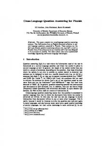
There are two stages in RDF Q/A systems: question understanding and query evaluation. Existing systems in the first stage translate a natural language question N into SPARQLs [29, 6, 13], and in the second stage evaluate all SPARQLs translated in the first stage. The focus of the existing solutions is on query understanding. Let us consider a running example in Figure 1. The RDF dataset is given in Figure 1(a). For the natural language question N “Who was married to an actor that played in Philadelphia ? ”, Figure 1(b) illustrates the two stages done in the existing solutions. The inherent hardness in RDF Q/A is the ambiguity of natural language. In order to translate N into SPARQLs, each phrase in N should map to a semantic item (i.e, an entity or a class or a predicate) in RDF graph G. However, some phrases have ambiguities. For example, phrase “Philadelphia” may refer to entity hPhiladelphia(film)i or hPhiladelphia_76ersi. Similarly, phrase “play in” also maps to predicates hstarringi or hplayForTeami. Although it is easy for humans to know the mapping from phrase “Philadelphia” (in question N ) to hPhiladelphia_76ersi is wrong, it is uneasy for machines. Disambiguating one phrase in N can influence the mapping of other phrases. The most common technique is the joint disambiguation [29]. Existing disambiguation methods only consider the semantics of a question sentence N . They have high cost in the query understanding stage, thus, it is most likely to result in slow response time in online RDF Q/A processing. In this paper, we deal with the disambiguation in RDF Q/A from a different perspective. We do not resolve the disambiguation problem in understanding question sentence N , i.e., the first stage. We take a lazy approach and push down the disambiguation to the query evaluation stage. The main advantage of our method is it can avoid the expensive disambiguation process in the question understanding stage, and speed up the whole performance. Our disambiguation process is integrated with query evaluation stage. More specifically, we allow that phrases (in N ) correspond

Subject

Predicate

Object

Antonio_Banderas

type

actor

Antonio_Banderas

spouse

Melanie_Griffith

Antonio_Banderas

starring

Philadelphia_(film)

Philadelphia_(film)

type

film

Jonathan_Demme Philadelphia

director type

Philadelphia_(film) city

bornIn

Philadelphia

Aaron_McKie James_Anderson

playedForTeam Philadelphia_76ers

Constantin_Stanislavski

create

An_Actor_Prepares

Philadelphia_76ers

type

Basketball_team

An_Actor_Prepares

type

Book

c1

Generating a Semantic Query Graph

Disambiguation

v1



Who

actor



play in



be married to “that”v2 play in



?who





film

u2 Antonio_Banderas



u1 Melanie_Griffith

u7 James_Anderson

u3 Philadelphia_(film) u4 Jonathan_Demme



SELECT ?y WHERE { ?x starring Philadelphia_ ( film ) . ?x type actor . ?x spouse ?y. }

Finding Top-k Subgraph Matches c1 actor

c4 Basketball_team

Query Evaluation u2

Antonio_Banderas



u10 Philadelphia_76ers u8 c5 Book Constantin_Stanislavski u10 An_Actor_Prepares (a) RDF Dataset and RDF Graph





u5 Philadelphia u6 Aaron_McKie

Philadelphia v3

actor



city

c2



Semantic Query Graph

be married to

Philadelphia

c3 actor

Who was married to an actor that play in Philadelphia ? SPARQL Generation



SPARQL Query Engine

u1 Melanie_Griffith

u3 Philadelphia_(film)

?y: Melanie_Griffith (b) SPARQL Generation-and-Query Framework

(c) Our Framework

Figure 1: Question Answering Over RDF Dataset to multiple semantic items (e.g., subjects, objects and predicates) in RDF graph G in the question understanding stage, and resolve the ambiguity at the time when matches of the query are found. The cost of disambiguation is saved if there are no matching found. In our problem, the key problem is how to define a “match” of question N in RDF graph G and how to find matches efficiently. Intuitively, a match is a subgraph (of RDF graph G) that can fit the semantics of question N . The formal definition of the match is given in Definition 3 (Section 2). We illustrate the intuition of our method by an example. Consider a subgraph of graph G in Figure 1(a) (the subgraph induced → by vertices u1 , u2 , u3 and c1 ). Edge − u− 2 c1 says that “Antonio Ban− − → deras is an actor”. Edge u2 u1 says that “Melanie Griffith is mar→ ried to Antonio Banderas”. Edge − u− 2 u3 says that “Antonio Banderas starred in a film hPhiladelphia(film)i”. The natural language question N is “Who was married to an actor that played in Philadel→ −−→ phia”. Obviously, the subgraph formed by edges − u− 2 c1 , u2 u1 and − − → u2 u3 is a match of N . “Melanie Griffith” is a correct answer. On the other hand, we cannot find a match (of N ) containing hPhiladelphia _76ersi in RDF graph G. Therefore, the phrase “Philadelphia” (in N ) cannot map to hPhiladelphia_76ersi. This is the basic idea of our data-driven approach. Different from traditional approaches, we resolve the ambiguity problem in the query evaluation stage. A challenge of our method is how to define a “match” between a subgraph of G and a natural language question N . Because N is unstructured data and G is graph structure data, we should fill the gap between two kinds of data. Therefore, we propose a semantic query graph QS to represent the question semantics of N . We formally define QS in Definition 2. An example of QS is given in Figure 1(c), which represents the semantic of the question N . Each edge in QS denotes a semantic relation. For example, edge v1 v2 denotes that “who was married to an actor”. Intuitively, a match of question N over RDF graph G is a subgraph match of QS over G (formally defined in Definition 3).

1.2

Our Approach

Although there are still two stages “question understanding” and “query evaluation” in our method, we do not adopt the existing framework, i.e., SPARQL generation-and-evaluation. We propose a graph data-driven solution to answer a natural language question

N . The coarse-grained framework is given in Figure 1(c). In the question understanding stage, we interpret a natural language question N as a semantic query graph QS (see Definition 2). Each edge in QS denotes a semantic relation extracted from N . A semantic relation is a triple hrel,arg1,arg2i, where rel is a relation phrase, and arg1 and arg2 are its associated arguments. For example, h“play in”,“actor”,“Philadelphia”i is a semantic relation. The edge label is the relation phrase and the vertex labels are the associated arguments. In QS , two edges share one common endpoint if the two corresponding relations share one common argument. For example, there are two extracted semantic relations in N , thus, we have two edges in QS . Although they do not share any argument, arguments “actor” and “that” refer to the same thing. This phenomenon is known as “coreference resolution” [25]. The phrases in edges and vertices of QS can map to multiple semantic items (such as entities, classes and predicates) in RDF graph G. We allow the ambiguity in this stage. For example, the relation phrase “play in” (in edge v2 v3 ) corresponds to three different predicates. The argument “Philadelphia” in v3 also maps to three different entities, as shown in Figure 1(c). In the query evaluation stage, we find subgraph matches of QS over RDF graph G. For each subgraph match, we define its matching score (see Definition 6) that is based on the semantic similarity of the matching vertices and edge in QS and the subgraph match in G. We find the top-k subgraph matches with the largest scores. For example, the subgraph induced by u1 , u2 and u3 matches query QS , as shown in Figure 1(c). u2 matches v2 (“actor”), since u2 (hAntonio_Banderasi) is a type-constraint entity and u2 ’s type is hactori. u3 (hPhiladelphia(film)i) matches v3 (“Philadelphia”) and u1 (hMelanie_Griffithi) matches v1 (“who”). The result to question N is hMelanie_Griffithi. Also based on the subgraph match query, we cannot find a subgraph containing u10 (hPhiladelphia_76ersi) to match QS . It means that the mapping from “Philadelphia” to u10 is a false alarm. We deal with disambiguation in query evaluation based on the matching result. Pushing down disambiguation to the query evaluation stage not only improves the precision but also speeds up the whole query response time. Take the up-to-date DEANNA [20] as an example. DEANNA [29] proposes a joint disambiguation technique. It mod-

Table 1: Notations Notation G(V, E) N Q Y D T rel vi /ui Cvi /Cvi vj d

Definition and Description RDF graph and vertex and edge sets A natural language question A SPARQL query The dependency tree of qN L The paraphrase dictionary A relation phrase dictionary A relation phrase A vertex in query graph/RDF graph Candidate mappings of vertex vi /edge vi vj Candidate mappings of vertex vi /edge vi vj

els the disambiguation as an ILP (integer liner programming) problem, which is an NP-hard problem. To enable the disambiguation, DEANNA needs to build a disambiguation graph. Some phrases in the natural language question map to some candidate entities or predicates in RDF graph as vertices. In order to introduce the edges in the disambiguation graph, DEANNA needs to compute the pairwise similarity and semantic coherence between every two candidates on the fly. It is very costly. However, our method avoids the complex disambiguation algorithms, and combines the query evaluation and the disambiguation in a single step. We can speed up the whole performance greatly. In a nutshell, we make the following contributions in this paper. 1. We propose a systematic framework (see Section 2) to answer natural language questions over RDF repositories from a graph data-driven perspective. To address the ambiguity issue, different from existing methods, we combine the query evaluation and the disambiguation in a single step, which not only improves the precision but also speed up query processing time greatly. 2. In the offline processing, we propose a graph mining algorithm to map natural language phrases to top-k possible predicates (in a RDF dataset) to form a paraphrase dictionary D, which is used for question understanding in RDF Q/A. 3. In the online processing, we adopt two-stage approach. In the query understanding stage, we propose a semantic query graph QS to represent the users’ query intention and allow the ambiguity of phrases. Then, we reduce RDF Q/A into finding subgraph matches of QS over RDF graph G in the query evaluation stage. We resolve the ambiguity at the time when matches of the query are found. The cost of disambiguation is saved if there are no matching found. 4. We conduct extensive experiments over several real RDF datasets (including QALD benchmark) and compare our system with some state-of-the-art systems. Experiment results show that our solution is not only more effective but also more efficient.

2.

FRAMEWORK

The problem to be addressed in this paper is to find the answers to a natural language question N over an RDF graph G. Table 1 lists the notations used throughout this paper. There are two key challenges in this problem. The first one is how to represent the query intention of the natural language question N in a structural way. The underlying RDF repository is a graph structured data, but, the natural language question N is unstructured data. To enable query processing, we need a graph representation of N . The second one is how to address the ambiguity of natural language phrases in N . In the running example, “Philadelphia” in the question N may refer to different entities, such as

ĂĂ

Figure 3: Paraphrase Dictionary D hPhiladelphia(film)i and hPhiladelphia_76ersi. We need to know which one is users’ concern. In order to address the first challenge, we extract the semantic relations (Definition 1) implied by the question N , based on which, we build a semantic query graph QS (Definition 2) to model the query intention in N . D EFINITION 1. (Semantic Relation). A semantic relation is a triple hrel, arg1, arg2i, where rel is a relation phrase in the paraphrase dictionary D, arg1 and arg2 are the two argument phrases. In the running example, h“be married to”, “who”,“actor”i is a semantic relation, in which “be married to” is a relation phrase, “who” and “actor” are its associated arguments. We can also find another semantic relation h“play in”, “that”,“Philadelphia”i in N . D EFINITION 2. (Semantic Query Graph) A semantic query graph is denoted as QS , in which each vertex vi is associated with an argument and each edge vi vj is associated with a relation phrase, 1 ≤ i, j ≤ |V (QS )| . Actually, each edge in QS together with the two endpoints represents a semantic relation. We build a semantic query graph QS as follows. We extract all semantic relations in N , each of which corresponds to an edge in QS . If the two semantic relations have one common argument, they share one endpoint in QS . In the running example, we get two semantic relations, i.e., h“be married to”, “who”,“actor”i and h“play in”, “that”,“Philadelphia”i, as shown in Figure 2. Although they do not share any argument, arguments “actor” and “that” refer to the same thing. This phenomenon is known as “coreference resolution” [25]. Therefore, the two edges also share one common vertex in QS (see Figure 2(c)). We will discuss more technical issues in Section 4.1. To deal with the ambiguity issue (the second challenge), we propose a data-driven approach. The basic idea is: for a candidate mapping from a phrase in N to an entity (i.e., vertex) in RDF graph G, if we can find the subgraph containing the entity that fits the query intention in N , the candidate mapping is correct; otherwise, this is a false positive mapping. To enable this, we combine the disambiguation with the query evaluation in a single step. For example, although “Philadelphia” can map three different entities, in the query evaluation stage, we can only find a subgraph containing hPhiladelphia_film i that matches the semantic query graph QS . Note that QS is a structural representation of the query intention in N . The match is based on the subgraph isomorphism between QS and RDF graph G. The formal definition of match is given in Definition 3. For the running example, we cannot find any subgraph match containing hPhiladelphiai or hPhiladelphia_76ersi of QS . The answer to question N is “Melanie_Griffith” according to the resulting subgraph match. Generally speaking, there are offline and online phases in our solution.

(a) Natural Language Question

1

3

Who

actor

1

2

(b) Semantic Relations Extraction and Building Semantic Query Graph

2

3

3 5 2

?who

4

6

1 7 9 8

5

An_Actor_Prepares

10

Figure 2: Natural Language Question Answering over Large RDF Graphs

2.1

Offline

To enable the semantic relation extraction from N , we build a paraphrase dictionary D, which records the semantic equivalence between relation phrases and predicates. For example, in the running example, natural language phrases “be married to” and “play in” have the similar semantics with predicates hspousei and hstarringi, respectively. Some existing systems, such as Patty [18] and ReVerb [10], provide a rich relation phrase dataset. For each relation phrase, they also provide a support set with entity pairs, such as (hAntonio_Banderasi, hPhiladelphia(film)i) for the relation phrase “play in”. Table 2 shows two sample relation phrases and their supporting entity pairs. The intuition of our method is as follows: for each relation phrase reli , let Sup(reli ) denotes a set of supporting entity pairs. We assume that these entity pairs also occur in RDF graph. Experiments show that more than 67% entity pairs in the Patty relation phrase dataset occur in DBpedia RDF graph. The frequent predicates (or predicate paths) connecting the entity pairs in Sup(reli ) have the semantic equivalence with the relation phrase reli . Based on this idea, we propose a graph mining algorithm to find the semantic equivalence between relation phrases and predicates (or predicate paths).

2.2

Online

There are two stages in RDF Q/A: question understanding and query evaluation. 1) Question Understanding. The goal of the question understanding in our method is to build a semantic query graph QS for representing users’ query intention in N . We first apply Stanford Parser to N to obtain the dependency tree Y of N . Then, we extract the semantic relations from Y based on the paraphrase dictionary D. The basic idea is to find a minimum subtree (of Y ) that contains all words of rel, where rel is a relation phrase in D. The subtree is called an embedding of rel in Y . Based on the embedding position in Y , we also find the associated arguments according to some linguistics rules. The relation phrase rel together with the two associated arguments form a semantic relation, denoted as a triple hrel,arg1,arg2i. Finally, we build a semantic query graph

QS by connecting these semantic relations. We will discuss more technical issues in Section 4.1. 2) Query Evaluation. As mentioned earlier, a semantic query graph QS is a structural representation of N . In order to answer N , we need to find a subgraph (in RDF graph G) that matches QS . The match is defined according to the subgraph isomorphism (formally defined in Definition 3) First, each argument in vertex vi of QS is mapped to some entities or classes in the RDF graph. Given an argument argi (in vertex vi of QS ) and an RDF graph G, entity linking [31] is to retrieve all entities and classes (in G) that possibly correspond to argi , denoted as Cvi . Each item in Cvi is associated with a confidence probability. In Figure 2, argument “Philadelphia” is mapped to three different entities hPhiladelphiai, hPhiladelphia(film)i and hPhiladelphia_76ersi, while argument “actor” is mapped to a class hActori and an entity hAn_ Actor_Preparesi. We can distinguish a class vertex and an entity vertex according to RDF’s syntax. If a vertex has an incoming adjacent edge with predicate hrdf:typei or hrdf:subclassi, it is a class vertex; otherwise, it is an entity vertex. Furthermore, if arg is a wh-word, we assume that it can match all entities and classes in G. Therefore, for each vertex vi in QS , it also has a ranked list Cvi containing candidate entities or classes. Each relation phrase relvi vj (in edge vi vj of QS ) is mapped to a list of candidate predicates and predicate paths. This list is denoted as Cvi vj . The candidates in the list are ranked by the confidence probabilities. It is important to note that we do not resolve the ambiguity issue in this step. For example, we allow that “Philadelphia” maps to three possible entities, hPhiladelphia_76ersi, hPhiladelphiai and hPhiladelphia(film)i. We push down the disambiguation to the query evaluation step. Second, if a subgraph in RDF graph can match QS if and only if the structure (of the subgraph) is isomorphism to QS . We have the following definition about match. D EFINITION 3. (Match) Consider a semantic query graph QS with n vertices {v1 ,...,vn }. Each vertex vi has a candidate list Cvi , i = 1, ..., n. Each edge vi vj also has a candidate list of Cvi vj ,

Joseph_P._Kennedy,_Sr.

hasChild

Table 2: Relation Phrases and Supporting Entity Pairs Relation Phrase “play in” “uncle of”

Supporting Entity Pairs (h Antonio_Banderas i, h Philadelphia(film) i), (h Julia_Roberts i, h Runaway_Bride i),...... (h Ted_Kennedy i, h John_F._Kennedy,_Jr. i) (h Peter_Corr i, h Jim_Corr i),......

where 1 ≤ i 6= j ≤ n. A subgraph M containing n vertices {u1 ,...,un } in RDF graph G is a match of QS if and only if the following conditions hold:

Ted_Kennedy

hasChild John_F._Kennedy

Antonio_Banderas

starring Philadelphia(film) (a) Āplay inā

hasChild hasGender Male

John_F._Kennedy,_Jr.

hasGender (b) Āuncle ofā

Figure 4: Mapping Relation Phrases to Predicates or Predicate Paths 1. If vi is mapping to an entity ui , i = 1, ..., n, ui must be in list Cvi ; and 2. If vi is mapping to a class ci , i = 1, ..., n, ui is an entity whose type is ci (i.e., there is a triple hui rdf:type ci i in RDF graph) and ci must be in Cvi ; and → −−→ u− 3. ∀vi vj ∈ QS ; − i uj ∈ G ∨ uj ui ∈ G. Furthermore, the −−→ −−→ predicate Pij associated with u i uj (or uj ui ) is in Cvi vj , 1 ≤ i, j ≤ n. Each subgraph match has a score, which is derived from the probability confidences of each edge and vertex mapping. Definition 6 defines the score, which we will discuss later. Our goal is to find all subgraph matches with the top-k scores. A TA-style algorithm [11] is proposed in Section 4.2.2 to address this issue. Each subgraph match of QS implies an answer to the natural language question N , meanwhile, the ambiguity is resolved. For example, in Figure 2, although “Philadelphia” can map three different entities, in the query evaluation stage, we can only find a subgraph (included by vertices u1 , u2 , u3 and c1 in G) containing hPhiladelphia_film i that matches the semantic query graph QS . According to the subgraph graph, we know that the result is “Melanie_Griffith”, meanwhile, the ambiguity is resolved. Mapping phrases “Philadelphia” to hPhiladelphiai or hPhiladelphia_76ersi of QS is false positive for the question N , since there is no data to support that.

3.

OFFLINE

The semantic relation extraction relies on a paraphrase dictionary D. A relation phrase is a surface string that occurs between a pair of entities in a sentence [17], such as “be married to” and “play in” in the running example. We need to build a paraphrase dictionary D, such as Figure 3, to map relation phrases to some candidate predicates or predicate paths. Table 2 shows two sample relation phrases and their supporting entity pairs. In this paper, we do not discuss how to extract relation phrases along with their corresponding entity pairs. Lots of NLP literature about relation extraction study this problem, such as Patty [18] and ReVerb [10]. For example, Patty [18] utilizes the dependency structure in sentences and ReVerb [10] adopts the n-gram to find relation phrases and the corresponding support set. In this work, we assume that the relation phrases and their support sets are given. The task in the offline processing is to find the semantic equivalence between relation phrases and the corresponding predicates (and predicate paths) in RDF graphs, i.e., building a paraphrase dictionary D like Figure 3. Suppose that we have a dictionary T = {rel1 , ..., reln }, where each reli is a relation phrase, i = 1, ..., n. Each reli has a support set of entity pairs that occur in RDF graph, i.e., Sup (reli ) = { (vi1 , vi01 ), ..., (vim , vi0m )}. For each reli , i = 1, ..., n, the goal is to mine top-k possible predicates or predicate paths formed by consecutive predicate edges in RDF graph, which have sematic equivalence with relation phrase reli .

Although mapping these relation phrases into canonicalized representations is the core challenge in relation extraction [17], none of the prior approaches consider mapping a relation phrase to a sequence of consecutive predicate edges in RDF graph. Patty demo [17] only finds the equivalence between a relation phrase and a single predicate. However, some relation phrases cannot be interpreted as a single predicate. For example, “uncle of” corresponds to a length-3 predicate path in RDF graph G, as shown in Figure 3. In order to address this issue, we propose the following approach. Given a relation phrase reli , its corresponding support set containing entity pairs that occurs in RDF graph is denoted as Sup(reli ) = { (vi1 , vi01 ), ..., (vim , vi0m )}. Considering each pair (vij , vi0j ), j = 1, ..., m, we find all simple paths between vij and vi0j in RDF S graph G, denoted as P ath(vij , vi0j ). Let P S(reli ) = j=1,...,m P ath(vij , vi0j ). For example, given an entity pair (h Ted_Kennedy i, h John_F._Kennedy,_Jr. i), we locate them at RDF graph G and find simple pathes between them (as shown in Figure 4). If a path L is frequent in P S(“uncle of”), L is a good candidate to represent the semantic of relation phrase “uncle of”. For efficiency considerations, we only find simple paths with no longer than a threshold1 . We adopt a bi-directional BFS (breathfirst-search) search from vertices vij and vi0j to find P ath(vij , vi0j ). Note that we ignore edge directions (in RDF graph) in a BFS process. For each relation phrase reli with m supporting entity pairs, we have a collection of all path sets P ath(vij , vi0j ), denoted as S P S(reli ) = j=1,...,m P ath(vij , vi0j ). Intuitively, if a predicate path is frequent in P S(reli ), it is a good candidate that has semantic equivalence with relation phrase reli . However, the above simple intuition may introduce noises. For example, we find that (hasGender , hasGender) is the most frequent predicate path in P S(“uncle of”) (as shown in Figure 4). Obviously, it is not a good predicate path to represent the sematic of relation phrase “uncle of”. In order to eliminate noises, we borrow the intuition of tf-idf measure [15]. Although (hasGender ,hasGender) is frequent in P S(“uncle of”), it is also frequent in the path sets of other relation phrases, such as P S(“is parent of”), P S(“is advisor of”) and so on. Thus, (hasGender ,hasGender) is not an important feature for P S(“uncle of”). It is exactly the same with measuring the importance of a word w with regard to a document. For example, if a word w is frequent in lots of documents in a corpus, it is not a good feature. A word has a high tf-idf, a numerical statistic in measuring how important a word is to a document in a corpus, if it occurs in a document frequently, but the frequency of the word in the whole corpus is small. In our problem, for each relation phrase reli , i = 1, ..., n, we deem P S(reli ) as a virtual document. All predicate paths in P S(reli ) are regarded as virtual words. The corpus contains all P S(reli ), i = 1, ..., n. Formally, we define tf-idf value of a predicate path L in the following definition. Note that if L is a length-1 predicate path, L is a predicate P . 1 We set the threshold as 4 in our experiments. More details about the parameter setting will be discussed in Section 6.

4.1 D EFINITION 4. Given a predicate path L , the tf-value of L in P S(reli ) is defined as follows: tf (L, P S(reli )) = |{P ath(vij , vi0j )|L ∈ P ath(vij , vi0j )}| The idf-value of L over the whole relation phrase dictionary T = {rel1 , ..., reln } is defined as follows: idf (L, T ) = log

|T | |{reli ∈ T |L ∈ P S(reli )}| + 1

The tf-idf value of L is defined as follows: tf−idf(L, P S(reli ), T ) = tf (L, P S(reli )) × idf (L, T ) We define the confidence probability of mapping relation phrase rel to predicate or predicate path L as follows. δ(rel, L) = tf−idf(L, P S(reli ), T )

(1)

Algorithm 1 Finding Predicate Path Patterns with Sematic Equivalence with Textual Patterns Require: Input: A relation phrase dictionary T = {rel1 , ..., reln } and each textural pattern reli , i = 1, ..., n, has a support set Sup(reli ) = { (vi1 , vi01 ), ..., (vim , vi0m )} and an RDF graph G. Output: Each relation phrase reli (i = 1, ..., n) has the top-k possible predicate path patterns {Li1 , ..., Lik } with the sematic equivalence with reli . 1: for each relation phrase reli , i = 1, ..., n in T do 2: for each entity pair (vij , vi0j ) in Sup(reli ) do 3: Find all simple predicate path patterns (with length less than a predefined parameter θ) between vij and vi0j , denoted as P ath(vij , vi0j ). S 4: P S(ti ) = j=1,....m P ath(vij , vi0j ) 5: for each relation phrase reli do 6: for each predicate path pattern L in P S(ti ) do 7: Compute tf-idf value of L (according to Definition 4) 8: for relation phrase reli , record the k predicate path patterns with the top-k highest tf-idf values.

Question Understanding

This subsection discusses how to identify semantic relations in a natural language question N , based on which, we build a semantic query graph QS to represent the query intention in N . In order to extract the semantic relations in N , we need to identify the relation phrases in question N . Obviously, we can simply regard the natural language question N as a sequence of words. The problem is to find which relation phrases (also regarded as a sequence of words) are subsequences of N . However, the ordering of words in a natural language sentence is not fixed, such as inverted sentences and fronting. For example, let us consider a question “In which movies did Antonio Banderas star ?”. Obviously, “star in” indicates the semantic relation between “Antonio Banderas” and “which movie”, but, “star in” is not a subsequence of the question language due to preposition fronting. The phenomenon is known as “long-distance dependency”. Some NLP (natural language processing) literature suggest that the dependency structure is more stable for the relation extraction [18]. The dependencies are grammatical relations between a governor (also known as a regent or a head) and a dependent. Usually, we can map straightforwardly these dependencies into a tree, called dependency tree [8]. Specifically, words in the sentence are corresponding to nodes in a dependency tree and the edge labels describe the grammatical relations. Note that “In which movies did Antonio Banderas star?” and “Which movies did Antonio Banderas star in ?” have the same dependency tree, even though the former has the preposition fronting phenomenon. Therefore, in our work, we first apply Stanford Parser [8] to N to obtain the dependency tree Y . Let us recall the running example. Figure 5 shows the dependency tree of N (in the running example), denoted as Y . The next question is to find which relation phrases occurring in Y . married nsubjpass

Who

Relation Extraction

prep

auxpass

was

to

R1=(“(be) married to”, “who”, “actor”)

pobj

R2=(“star in”, “that”, “Philadelphia”)

actor

Algorithm 1 shows the details of finding top-k predicate paths for each relation phrase. All relation phrases and their corresponding k predicate paths including tf-idf values are collected to form a paraphrase dictionary D. Note that the tf-idf is a probability value to evaluate the mapping (from relation phrase to predicate/predicate paths) confidence. To maintain the dictionary D, we can just re-mine the mappings for newly introduced predicates, or delete all mappings for the predicates when they are removed from the dataset. More details about the maintenance issue can be found at the full version of this paper [1]. T HEOREM 1. The time complexity of Algorithm 1 is O(|T | × |V |2 × d2 ), where |T | is the number of relation phrases in T , |V | is the number of vertices in RDF graph G, and d is the maximal vertex degree. We omit the proof due to space constraints.

4.

ONLINE

The online processing consists of two stages: question understanding and query evaluation. In the former one, we need to translate a natural language question N to a semantic query graph QS . Then, in the second stage, we find subgraph matches of QS . We resolve the ambiguity of natural language phrases at the time when the matches are found.

Relation Extraction

rcmod

det

an

starred nsubj

that

prep

in pobj

Philadelphia

Figure 5: Relationship Extraction D EFINITION 5. Let us consider a dependency tree Y of a natural language question N and a relation phrase rel. We say that rel occurs in Y if and only if there exists a connected subtree y (of Y ) satisfying the following conditions: 1. Each node in y contains one word in rel and y includes all words in rel. 2. We cannot find a subtree y 0 of Y , where y 0 also satisfies the first condition and y is a subtree of y 0 . In this case, y is an embedding of relation phrase rel in Y . Given a dependency tree Y of a natural language question N and a relation phrase dictionary T = {rel1 , ..., reln }, we need to find which relation phrases (in T ) are occurring in Y . Let us consider Figure 5. The dependency tree Y of the natural language in the running example is given in Figure 5. We find two

Algorithm 2 Finding Relation Phrases Occurring in a Natural Language Questions N Require: Input: A dependency tree Y and an inverted index over the relation phrase dictionary T . Output: All embeddings of relation phrases (in T ) occurring in Y . 1: for each node wi in Y do 2: Find a list of relation phrases P Li occurring in T by the inverted list. 3: for each node wi in Y do 4: Set P L = P Li 5: for each relation phrase rel ∈ P L do 6: Set rel[wi ] = 1 // indicating the appearance of word wi in rel. 7: Call Probe(wi , P L) 8: for each relation phrase rel in P Li do 9: if all words w of rel have rel[w] = 1 then 10: rel is an occurring relation phrase in Y 11: Return rel and a subtree rooted at wi includes (and only includes) all words in rel. Probe(w, P L0 ) 1: for each child w0 of w do 2: P L00 = P L0 ∩ P Li . 3: if P L00 == φ then 4: return 5: else 6: for each relation phrase rel ∈ P L00 do 7: Set rel[w0 ] = 1 // indicating the appearance of word w0 in t. 8: Call Probe(w0 , P L00 )

relation phrases rel1 =“be married to” and rel2 =“star in” occurring in Y , where rel1 and rel2 are in a paraphrase dictionary T . We also find their associated arguments of rel1 and rel2 , respectively. Finally, we can find two relations R1 and R2 in this example, which are denoted as the triple representation (as shown in Figure 5). Now, we discuss how to find relation phrase embeddings and the associated arguments as follows.

4.1.1

Finding Relation Phrase Embeddings

Given a natural language question N , we propose an algorithm (Algorithm 2) to identify all relation phrases in N . In the offline phase, we build an inverted index over all relation phrases in the paraphrase dictionary D. Specifically, for each word, it links to a list of relation phrases containing the word. At run time, we first get the dependency tree Y of a natural language question N . In order to find relation phrases occurring in Y , we propose Algorithm 2. The basic idea is as follows: For each node (i.e., a word) wi in Y , we find the candidate pattern list P Li (Steps 1-2 in Algorithm 2). Then, for each node wi , we check whether there exists a subtree rooted at wi including all words of some relation phrases in P Li . In order to address this issue, we propose a depth-first search strategy. We probe each path rooted at wi (Step 3). The search branch stops at a node w0 , where there does not exists a relation phrase including w0 and all words along the path between w0 and wi (Note that, w0 is a descendant node of wi .)(Lines 3-4 in Probe function.) We utilize rel[w] to indicate the presence of word w of rel in the subtree rooted at wi (Line 6). When we finish all search branches, if rel[w] = 1 for all words w in relation phrase rel, it means that we have found a relation phrase rel occurring in Y and the embedding subtree is rooted at wi (Lines 8-11). We can find the exact embedding (i.e., the subtree) by probing the paths rooted at wi . We omit the trivial details due to the space limit. T HEOREM 2. The time complexity of Algorithm 2 is O(|Y |2 ).

4.1.2

Finding Associated Arguments

After finding a relation phrase in Y , we then look for the two associated arguments. Generally, the arguments arg1 and arg2 are

recognized mainly based on the grammatical subject-like and objectlike relations around the embedding, which are listed as follow 2 : 1. subject-like relations: subj, nsubj, nsubjpass, csubj, csubjpass, xsubj, poss; 2. object-like relations: obj, pobj, dobj, iobj Assume that we find an embedding subtree y of a relation phrase rel. We recognize arg1 by checking for each node w in y whether there exists the above subject-like relations (by checking the edge labels in the dependency tree) between w and one of its children (note that, the child is not in the embedding subtree). If a subjectlike relationship exists, we add the child to arg1. Likewise, arg2 is recognized by the object-like relations. When there are still more than one candidates for each argument, we choose the nearest one to rel. On the other hand, when arg1/arg2 is empty after this step, we introduce several heuristic rules (based some computational linguistics knowledge) to increase the recall for finding arguments. The heuristic rules are applied until arg1/arg2 becomes none empty. • Rule 1: Extend the embedding t with some light words, such as prepositions, auxiliaries. Recognize subject/object-like relations for the newly added tree node. • Rule 2: If the root node of t has subject/object-like relations with its parent node in Y , add the root node to arg1. • Rule 3: If the parent of the root node of t has subject-like relations with its child, add the child to arg1. • Rule 4: If one of arg1/arg2 is empty, add the nearest wh-word (such as what, who and which) or the first noun phrase in t to arg1/argu2. If we still cannot find arguments arg1/arg2 after applying the above heuristical rules, we just discard the relation phrase rel in the further consideration. Finally, we can find all relation phrases occurring in N together with their embeddings and their arguments arg1/arg2. Let us recall dependency tree Y in Figure 5. There is a “nsubjpass” dependency between “who” and a relation phrase “(be) married to”. Thus, the first argument is “who”. Analogously, we can find another argument “actor” based on the “pobj” dependency. Therefore, the first semantic relation is h“(be) married to”, “who”, “actor”i. Likewise, we can also find another semantic relation h“play in”, “that”, “Philadelphia”i.

4.1.3

Building Semantic Query Graph

After obtaining all semantic relations in a natural language N , we need to build a semantic query graph QS . Actually, a semantic query graph is a structural representation of users’ query intention. Figure 2(b) shows an example of QS . In order to build a semantic query graph QS , the method is as follows. We represent each semantic relation hrel, arg1, arg2i as an edge. Two edges share one common endpoint if their corresponding semantic relations have one common argument. The formal definition of a query semantic graph has been given in Definition 2. Let us recall the running example. Although two relations h“be married to”, “who”, “actor”i and h“play in”, “that”, “Philadelphia”i do not share any argument, “actor” and “that” actually refer to the same thing. This phenomenon is known as “coreference resolution” [25]. Therefore, the two corresponding edges share an endpoint (“actor” and “that”) in QS , as shown in Figure 2(b). Note that 2 These grammatical relationships (called dependencies) that are defined in [8]. For example, “nsubj” refers to a nominal subject. It is a noun phrase which is the syntactic subject of a clause. Interested reader can refer to [8] for more details.

we can utilize the existing solutions to address the “coreference resolution”. This problem has been well studied in natural language processing [25].

4.2 4.2.1

Query Evaluation Phrases Mapping

The semantic query graph QS plays an important role in answering the natural language question N . Actually, QS bridges the gap between users’ un-structured query intention of a natural language question N and the structured RDF data G. There are two different items in QS . One is the relation phrase in each edge of QS . The other one is the argument in each vertex of QS . In this subsection, we discuss how to map the relation phrases and arguments to candidate predicates/predicate paths and entities/classes, respectively. Mapping Edges of QS . Each edge vi vj in QS has a relation phrase relvi vj . According to the paraphrase dictionary D (see Section 3), it is straightforward to map relvi vj to some predicates P or predicate paths L. The list is denoted as Cvi vj . As mentioned earlier, P is a special case when L’s length is one. For simplicity of notations, we use L in the following discussion. Each mapping is associated with a confidence probability δ(rel, L) (defined in Equation 1). For example, edge v2 v3 has a relation phrase relv2 v3 =“play in”. Its candidate list Cv2 v3 contains three candidates, hplayForTeami, hstarringi, and hdirectori, as shown in Figure 2(c). We also record the confidence probability δ(rel, L) in Cv2 v3 . Note that we allow the ambiguity in the mapping in this stage. Mapping Vertices of QS . Let us consider any vertex v in QS . The argument associated with v is arg. If arg is a wh-word, it can be mapped to all entities and classes in RDF graph G. Otherwise, given an argument arg, we should return a list of corresponding entities or classes. This is an entity linking problem [16, 21]. We use notation Cv to denote all candidates with regard to vertex v in QS . For example, argument “Philadelphia” in v3 (in Figure 2) is linked to three different entities in RDF graph, i.e., hPhiladelphiai, hPhiladelphia(film)i and hPhiladelphia_76ersi. “actor” in v2 can be linked to a class node hactori or an entity node “An_Actor_Prepares”. The entity linking problem is well studied in the literature, such as Wikify [16] and Wikifier [21]. In this work, we use an existing system, DBpedia Lookup [4] 3 , to return a list of corresponding entities and classes for an argument. If arg is mapped to an entity u, we use δ(arg, u) to denote the confidence probability; if arg is mapped to a class c, we use δ(arg, c) to denote the confidence probability. As mentioned earlier, in our method, we do not address the disambiguation issue in this stage. Graph Data-driven Disambiguation. Obviously, there are some ambiguity problems in the above mapping process. For example, “Philadelphia” in the natural language question N can be mapped to three different entities, i.e., hPhila delphia(film)i, hPhiladelphiai and hPhiladelphia_76ersi. In this work, we regard the disambiguation from another perspective—graph data-driven solution. We allow the ambiguity in the phrase mapping step and push down the disambiguation into the query evaluation stage. Assume that a vertex v in QS maps to lots of candidate vertices in RDF graph G. If a candidate is in a match (see Definition 3) of QS in RDF graph G, it is a reasonable candidate. Furthermore, the subgraph is an answer to the natural language question N . Otherwise, the candidate is a false positive.

4.2.2

Given a semantic query graph QS , we discuss how to find topk subgraph matches over RDF graph G in this subsection. The formal definition of a subgraph match is given in Definition 3 (in Section 2.2). Each vertex vi in QS has a list Cvi of candidate vertices (i.e., entities and classes) in RDF graph G. Assume that vi in QS has an argument argi . For any candidate vertex ui in Cvi , we use δ(argi , ui ) to denote the confidence probability. Analogously, each edge vi vj in QS also has a list Cvi vj of candidate predicates in G. Assume that edge vi vj has a relation phrase relvi vj . For any candidate predicate Pij in Cvi vj , we use δ(relvi vj , Pij ) to denote the confidence probability. We assume that all candidate lists are ranked in the non-ascending order of the confidence probability. Figure 2(b) and (c) show an example of QS and the candidate lists, respectively. Each subgraph match of QS has a score. It is computed from the confidence probabilities of each edge and vertex mapping. The score is defined as follows. D EFINITION 6. Given a semantic query graph QS with n vertices {v1 ,...,vn }, a subgraph M containing n vertices {u1 ,...,un } in RDF graph G is a match of QS . The match score is defined as follows: Score(M Q )= Q log( vi ∈V (QS ) δ(argi , ui ) × vi vj ∈E(QS ) δ(relvi vj , Pij )) P P = vi ∈V (QS ) log(δ(argi , ui )) + vi vj ∈E(QS ) log(δ(relvi vj , Pij )) (2) where argi is the argument of vertex vi , and ui is an entity or a class in RDF graph G, and relvi vj is the relation phrase of edge → −−→ vi vj and Pij is a predicate of edge − u− i uj or uj ui . Given a semantic query graph QS , our goal is to find all subgraph matches of QS (over RDF graph G) with the top-k match scores 4 . This is an NP-hard problem. We provide the detailed analysis as follows. L EMMA 1. Finding Top-1 subgraph match of QS over RDF graph G is an NP-hard problem. P ROOF. As we know, the decision problem of subgraph isomorphism is a classical NP-complete problem. We can reduce the decision problem of subgraph isomorphism to finding top-1 subgraph match of QS over G in a polynomial time, since the former can be solved by invoking the latter problem. It means finding the top-1 subgraph is at least as hard as subgraph isomorphism problem. Since subgraph isomorphism problem is an NP complete problem, it means that finding the top-1 subgraph is an NP-hard problem. L EMMA 2. Finding Top-k subgraph match of QS over RDF graph G is at least as hard as finding Top-1 subgraph match of QS over G. P ROOF. We can reduce finding top-1 subgraph match to finding top-k subgraph matches, since the former can be solved by invoking the latter problem. When we find top-k subgraph matches, we can find the top-1 in O(k) time. It means that finding top-k subgraph match is at least as hard as finding top-1 subgraph match. T HEOREM 3. Finding Top-k subgraph matches of QS over RDF graph G is an NP-hard problem. 4

3

http://lookup.dbpedia.org/api/search.asmx

Finding top-k Subgraph Matches

Note that if more than one match have the identical score in the top-k results, they are only counted once. In other words, we may return more than k matches if some matches share the same score

P ROOF. It can be derived from Lemmas 1 and 2. Since finding top-k subgraph matches is an NP-hard problem, hence, we concentrate on designing heuristic rules to reduce the search space. The first pruning method is to reduce the candidates of each list (i.e, Cvi and Cvi vj ) as many as possible. If a vertex ui in Cvi cannot be in any subgraph match of QS , ui can be filtered out directly. Let us recall Figure 2. Vertex u5 is a candidate in Cv3 . However, u5 does not have an adjacent predicate that is mapping to phrase “play in” in edge v2 v3 . It means that there exists no subgraph match of QS containing u5 . Therefore, u5 can be pruned safely. This is called neighborhood-based pruning. It is often used in subgraph search problem, such as [32].

Table 4: Statistics of RDF Graph Number of Entities Number of Triples Number of Predicates Size of RDF Graphs (in GB)

DBpedia 5.2 million 60 million 1643 6.1

Table 5: Statistics of Relation Phrase Dataset Number of Textual Patterns Number of Entity Pairs Average Entity Pair Number For Each Pattern

wordnet-wikipedia 350,568 3,862,304 11

freebase-wikipedia 1,631,530 15,802,947 9

Algorithm 3 Generating Top-k SPARQL Queries

5.

Require: Input: A semantic query graph QS and a RDF G. Output: Top-k SPARQL Queries, i.e., the top-k matches from QS to G. 1: for each candidate list Lri , i = 1, ......, |E(QS )| do 2: Sorting all candidate relations in Lri in a non-ascending order 3: for each candidate list Largj , j = 1, ......, |V (QS )| do 4: Sorting all candidate entities/classes (i.e., vertices in G0 ) in Largj in a non-ascending order. 5: Set cursor ci to the head of Lri and cursor cj to the head of Largj , respectively. 6: Set the upper bound U pbound(Q) according to Equation 3 and the threshold θ = −∞ 7: while true do 8: for each cursor cj in list Largj , j = 1, ......, |V (QS )| do 9: Performance a exploration based subgraph isomorphism algorithm from cursor cj , such as VF2, to find subgraph matches (of QS over G), which contains cj . 10: Update the threshold θ to be the top-k match sore so far. 11: Move all cursors ci and cj by one step forward in each list. 12: Update the upper bound U pbound(Q) according to Equation 3. 13: if θ ≥ U pbound(Q) then 14: Break // TA-style stopping strategy

In the offline phase, we need to build a paraphrase dictionary D by Algorithm 1. Therefore, the time complexity of the offline phase (Algorithm 1) is O(|T | × |V |2 × d), where |T | is the number of relation phrases, |V | is the number of vertices in RDF graph G, d is the largest vertex degree. In the online phase, there are two stages, i.e., question understanding and query evaluation. The first stage consists of four steps. Given a natural language question N , we obtain a dependency tree Y by the dependency parser. As we know, the time complexity of the dependency parser is O(|Y |3 ) [5], such as Eisner’s algorithm [9]. The second step is to find all relation embeddings by Algorithm 2, whose time complexity is O(|Y |2 ). The last two substeps (finding associated arguments and building semantic query graph) are linear with the number of relation phrases in N . It is straightforward to know there are at most |Y | relation phrases, i.e., assuming each word in N is a relation phrase. Therefore, the whole time complexity of the question understanding in our method is O(|Y |3 ). In the second stage, “query evaluation”, our method needs to find subgraph matches of the semantic query graph over RDF graph G. It includes two sub steps, i.e., finding phrases mappings (Section 4.2.1) and finding subgraph matches (Section 4.2.2). Obviously, the time complexity of this stage is NP-hard due to the time complexity of finding subgraph matches (see Theorem 3). Table 3 summarizes the time complexity of each step.

The second method is to stop the search process based on the top-k match score threshold as early as possible. We perform a TAstyle algorithm to find the top-k matches. The pseudo codes are given in Algorithm 3. There is a cursor for each candidate list. For each vertex vi in QS , we set cursor pi point to list Cvi . For each edge vi vj in QS , we also set cursor pij to list Cvi vj . For ease of presentation, we also use pi to denote the vertex (in G) that cursor pi points to, when the context is clear. Initially, all cursors point to the heads of candidate lists. We maintain a threshold θ to be the k-th highest score so far. It is −∞ at the beginning. For each pi , i = 1, ..., |V (QS )|, we perform a subgraph isomorphism algorithm (such as VF2 algorithm [7]) from vertex pi (in G) to find subgraph matches containing vertex pi . We probe each pi in a round-robin manner, i = 1, ..., |V (QS )|. Then, we update the current threshold θ according to the scores of these newly discovered matches. The upper bound for undiscovered matches is computed by the following equation. U pbound =

X pi

log(δ(argi , pi )) +

X

log(δ(relvi vj , pij )) (3)

pij

where pi denotes the current entity/class in the list Cvi and pij denotes the current predicate in the list Cvi vj . If the threshold θ > U pbound, it means that the score of all undiscovered matches cannot be higher than the current top-k match score. In other words, we have found the top-k matches. Thus, we can terminate the algorithm. Otherwise, we move all cursors one step forward and iterate the above steps.

6.

TIME COMPLEXITY ANALYSIS

EXPERIMENTS

In this section, we compare our method with one state-of-the-art algorithm DEANNA [29] and all systems in QALD-3 competition on DBpedia RDF dataset. To build the paraphrase dictionary, we utilize relationship phrases in Patty [18] system. All experiments are implemented in a PC server with Intel Xeon CPU 2GB Hz, 32GB memory and 3T disk running Windows 2008. We also evaluate our method in other RDF repositories, such as Yago2. Due to the space limit, we only report the experiment results on DBpedia.

6.1

Datasets

DBpedia RDF repository (http://blog.dbpedia.org/) is a community effort to extract structured information from Wikipedia and to make this information available on the Web [4]. The statistics of the RDF dataset are given in Table 4. Patty relation phrase dataset [18] contains a large resource for textual patterns that denote binary relations between entities. We use two different relation phrase datasets, wordnet-wikipedia and freebase-wikipedia, in our experiments. The former has 350,568 relation phrases and the latter has 1,631,530 relation phrases. For each relation phrase, Patty also provides a set of supporting entity pairs. More details can be found at Table 5.

Table 3: Time Complexity of Each Step in Our Method Offline Building Paragraph Dictionary

O(|T | × |V |2 × d2 )

Online building dependency tree O(|Y |3 )

Question Understanding finding relation finding arguembedding ments

build QS

Phrase mapping

Query Evaluation Subgraph matching

O(|Y |2 )

O(|Y |)

O(|V | + |E|)

NP-hard

O(|Y |)

Table 6: A Sample of Textual Patterns and Predicates/Predicate Paths in DBpedia

Table 7: Running Time of Offline Processing wordnet-wikipedia freebase-wikipedia

6.2

θ=2 17 mins 119 mins

θ=4 3.88 hrs 30.33 hrs

Offline Performance

Exp 1. Precision of Paraphrase Dictionary. In this experiment, we evaluate the accuracy of our building paraphrase dictionary method. For each relation phrase, we output a list of predicates/predicate paths. They are ranked in the non-descending order of confidence probabilities. Table 6 shows a sample of outputs in DBpedia. Note that the confidence probabilities in Tables 6 are normalized. In order to measure the accuracy, we perform the following experiments. We randomly select 1000 relation phrases from wordnetwikipedia and freebase-wikipedia datasets, respectively. For each relation phrase, we output top-3 corresponding predicates/predicate paths. These results are shown to human judges. For each relation phrase and its corresponding predicate/predicate path, the judge has to decide a scale from 2 to 0. The result is correct and highly relevant(2), correct but less relevant (1), or irrelevant (0). We find the precision (P@3) is about 50% when the path length is 1. However, while increasing of path length (from 2 to 4), the precision goes down greatly. To guarantee the precision of the paraphrase dictionary for online process, the top-3 predicate paths (for each relation phrase) should go through a human verification process. To further improve the precision of mapping relation phrases to predicate paths, a supervised learning and constraint-based path finding is a possible technique to be explore, which we will study as our future work. Exp 2. Running Time of Offline Processing. In this experiment, we evaluate the efficiency of our approach. Table 7 shows the total offline time. For example, when the path length threshold θ = 2, the running time is 17 minutes using wordnet-wikipedia relation phrase dataset and DBpedia RDF graph. Obviously, with the increasing of path length, the running time is increasing as well. On the other hand, with the increasing of path length, the precision of the results is decreasing. As default, we set θ = 4. The predicate paths with length longer than 4 will not be considered in our method.

6.3

Online Performance

QALD is the only benchmark for the RDF Q/A problem. It includes both the underling RDF knowledge base and the natural language questions. QALD is based on DBpedia knowledge base. To enable the comparison with other systems in QALD-3 competition, we report the experiment results in QALD-3 format in Table 8. We also compare with one state-of-the-art algorithm DEANNA [29] in our experiments. In our experiments, we set k = 10 in finding top-k subgraph matches. If all top-10 results are correct, we say that we correctly answer the questions. The gold standards of QALD-3 are provided by the organizers of the QALD competition. Note that some questions have less than 10 results. In this case, if all results reported by our system are correct, we say that we correctly answer the questions. Exp 3. (End-to-End Performance) We use all QALD-3 test queries (99 questions) in our experiments. We show the experiment results in QALD-3 result format (in Tables 8) to enable the comparison with all systems in QALD-3 (the experiment result of QALD-3 campaign is available at 5 ). We also compare with DEANNA [29] and report the experiment results in Table 8. We report the query result (i.e., precision, recall, F-measure) of each question in the same format with QALD-3 result format in the full version of this paper [1]. Effectiveness Evaluation. Our method can answer 32 questions correctly. We report the 32 questions in Table 11 together with the total response time in our method. Furthermore, our system can answer 11 questions partially. DEANNA [29] can only answer 21 questions correctly. Our system can beat all systems in QALD3 campaign in precision except for squall2sparql. Although the best system in QALD-3 campaign is squall2sparql, which can answer 77 questions, the input to squall2sparql is a controlled English question rather than a natural language question. Users need to specify the precise entities and predicates (denoted by URIs) in the question. For example, “Who is the dbp:father of res:Elizabeth II?” is an example input to squall2sparql system. In the question, “dbp:father” and “res:Elizabeth II” are URIs of the corresponding predicates and entities. Obviously, it is different from the traditional Q/A system. Therefore, we do not compare our method with squall2sparql. The second best system, CASIA, can answer 30 queries correctly [6]. More details are shown in Table 8. Efficiency Evaluation. We compare the running time of our approach with DEANNA [29] and CASIA. Due to the space limit, we only report the comparison with DEANNA in Figure 6. We test all questions that can be answered by both DEANNA and our method. In the question understanding, DEANNA needs to generate SPARQLs, our system generates semantic query graph Qs . The former has the exponential time complexity, but our method has the polynomial time complexity in the question understanding stage, as discussed in Section 5. The experiment results in Figure 6 confirm that generating SPARQLs is an expensive operation, since it needs to address the disambiguation issue. The question understanding of DEANNA often needs a few of seconds in our 5 http://greententacle.techfak.uni-bielefeld.de/ ~cunger/qald/3/qald3_results.pdf

Table 8: Evaluating QALD-3 Testing Questions (on DBpedia) Our Method squall2sparql CASIA Scalewelis RTV Intui2 SWIP DEANNA

Processed Right 76 32

Partially Recall Precision 11 0.40 0.40

F-1 0.40

96 52 70 55 99 21 27

13 8 38 4 4 2 0

0.87 0.36 0.33 0.33 0.32 0.16 0.21

77 29 1 30 28 14 21

0.85 0.36 0.33 0.34 0.32 0.15 0.21

0.89 0.35 0.33 0.32 0.32 0.16 0.21

Running Time (in ms)

100000

10000

1000

100

10 Q2 Q20 Q21 Q22 Q28 Q35 Q41 Q42 Q44 Q45 Q54 Q74 Q76 Q83 Q84 Q86 Question Understanding in DEANNA

Question Understanding in Our System

Overall time in DEANNA

Overall time in Our System

Figure 6: Online Running Time Comparison experiments. However, our method only spends no more than 100 ms in the question understanding stage (i.e., generating semantic query graph). Furthermore, the total response time of our method is faster than DEANNA by 2-68 times. Exp 4. (Evaluating Heuristic Rules For Finding Associated Arguments) In this experiment, we evaluate the effectiveness of the four heuristic rules in Section 4.1.2. In Table 9, we show the effects of the four heuristic rules on finding associated arguments. We also report the number of questions that can be answered correctly in our method using the four rules or without the four rules in Table 9. Table 9 shows that we can find the associated arguments in 48 questions correctly if using the four rules, but, the number is 32 without using the four rules. Table 9 also shows that we can answer more questions correctly using the four rules than without using that. Thus, the four heuristic rules can help improve the precision of our method. Exp 5. (Failure Analysis) We provide the failure analysis of our method. There are three key reasons for the failure of some questions in our method. The first reason is the named entity linking problem. For example, “In which UK city are the headquarters of the MI6 ”. We fail in linking MI6 to the corresponding entity. The second one is the failure of the semantic relation extraction. The third one is that our method cannot answer some aggregation (such as Max/Min) questions. They should be translated to SPARQLs with FILTER, like “ORDER BY DESC(?x) OFFSET 0 LIMIT 1”. We give the ratio of each reason in Table 10. Also, we give an example of each reason in Table 10. The failure analysis will help the improvement of our RDF Q/A system’s precision.

7.

RELATED WORK

Q/A (natural language question answering) has a quite long history since the seventies of last century [24]. Compared to keyword search, users can imply semantic relationships between the keywords using a whole sentence. Generally, there are three different categories of QA systems: (1) Text-based QA systems [20, 22] first retrieve a set of documents that are most relevant to the question, and then extract the answers from these documents. (2) Collaboration-based QA systems [28] exploit answers from the similar questions which have been answered by users on collaborative

Table 9: Evaluating The Heuristic Rules finding arguments correctly answering questions correctly

without the four rules 32

using the four rules 48

21

32

Table 10: Failure Analysis Reason Entity Linking Failure Relation Extraction Failure Aggregation Query Others

#(Ratio) 17 (27%) 14 (22%) 22 (35%) 10 (16%)

Sample Example Q48: In which UK city are the headquarters of the MI6? Q64. Give me all launch pads operated by NASA. Q13. Who is the youngest player in the Premier League? Q37. Give me all sister cities of Brno.

QA platforms, such as Yahoo! Answer and Quora. (3) Structureddata-based QA systems find answers by searching the database instead of the corpus, where the natural language questions are usually translated into some structural queries, such as SQL [19], SPARQL [29, 27] and others [3]. [27] pareses the questions to SPARQL templates, and instantiate the templates by entity/predicate mapping. DEANNA [29] builds a disambiguation graph and reduces disambiguation as an integer linear programming problem. Our work belongs to the third category and differs from previous work in three points. First, different from [27], our method does not adopt any manually defined SPARQL templates. Second, different from most existing RDF Q/A systems, such as [27] and DEANNA [29], we push down the disambiguation into the query evaluation stage. Existing solutions, like [27] and [29], generate the SPARQLs as the intermediate results in the question understanding stage. Obviously, they need to do disambiguation in this step. For example, DEANNA [29] proposes an integer linear programming (ILP)-based method to address the disambiguation issue. As we know, ILP is a classical NP-hard problem. Then, in the query evaluation stage, the existing methods need to answer these generated SPARQL queries. Answering SPARQL queries equals to finding subgraph matches of query graphs Q over RDF graph [33], which is also an NP-hard problem. We compare our method with one state-of-the-art method DEANNA in [29] from the complexity viewpoint. Table 12 shows the time complexity of each stage in both DEANNA and our method. The time complexity of the question understanding stage in our method is polynomial, but it is NP-hard in [29]. Generally speaking, although both [29] and our method are NP-hard in the online phrase (since the query evaluation stage dominates the whole complexity), our method is much faster than [29] in practice. The complexity of our method lies in finding subgraph matches. However, lots of literatures discuss the optimization methods for subgraph search [32, 26]. Therefore, our method has better performance than existing work. The comparison experiment results have been given in Exp 4 (in Section 6.3) and Table 7. Although the idea of combining disambiguation and query evaluation together has been considered recently, such as [12] for keyword search and [23] for entity search over the textural corpus, their problem definitions are different from ours. We focus on the natural language question answering on RDF repositories. Third, our method can consider answer some questions that contains the semantic relationships which are represented by a path in the RDF graph, rather than a single edge. However, existing systems, such as [33] and DEANNA [29], only consider mapping the relation phrase to single predicates. Furthermore, there are some work studying finding paths satisfying a regular expression between two vertices [14]. Note that this

Table 11: The QALD-3 Questions that can be Answered Correctly in Our System ID

Questions

Q2 Q3 Q14 Q17 Q19

Who was the successor of John F. Kennedy? Who is the mayor of Berlin? Give me all members of Prodigy? Give me all cars that are produced in Germany ? Give me all people that were born in Vienna and died in Berlin ? Q20 How tall is Michael Jordan ? Q21 What is the capital of Canada ? Q22 Who is the governor of Wyoming ? Q24 Who was the father of Queen Elizabeth II? Q27 Sean Parnell is the governor of which U.S. state ? Q28 Give me all movies directed by Francis Ford Coppola. Q30 What is the birth name of Angela Merkel ? Q35 Who developed Minecraft ?. Q39 Give me all companies in Munich. Q41 Who founded Intel? Q42 Who is the husband of Amanda Palmer ? Q44 Which cities does the Weser flow through ? Q45 Which countries are connected by the Rhine ? Q54 What are the nicknames of San Francisco ? Q58 What is the time zone of Salt Lake City ? Q63 Give me all Argentine films. Q70 Is Michelle Obama the wife of Barack Obama ? Q74 When did Michael Jackson die ? Q76 List the children of Margaret Thatcher. Q77 Who was called Scarface? Q81 Which books by Kerouac were published by Viking Press ? Q83 How high is the Mount Everest ? Q84 Who created the comic Captain America ? Q86 What is the largest city in Australia ? Q89 In which city was the former Dutch queen Juliana buried ? Q98 Which country does the creator of Miffy come from ? Q100 Who produces Orangina ?

Response Time (in ms) 1699 677 811 297 2557 942 1342 796 538 1210 577 250 2565 1312 1105 1418 1139 736 321 316 427 316 258 1139 719 796

University) for some efforts in the experiments. Authors are also grateful to anonymous reviewers for their constructive comments.

9.[1] Natural REFERENCES language question answering over rdf. In technique report, omitted due [2] [3] [4]

[5] [6]

[7]

[8] [9] [10] [11] [12] [13] [14] [15] [16]

635 589 1419 1700

[17] [18] [19]

2121 367 [20]

Table 12: Online Time Complexity Comparison Different proaches Our Method DEANNA [28]

Ap-

Online [21] Question Understanding O(|V |3 ) NP-hard (ILP problem)

Query Evaluation NP-hard NP-hard

is different from our path finding problem, since we focus on finding all simple paths between a pair of vertices under the path length constraint θ.

8.

CONCLUSIONS

In this paper, we propose a whole graph data-driven framework to answer natural language questions over RDF graphs. Different from existing work, we allow the ambiguity in the question understanding stage. We push down the disambiguation into the query evaluation stage. Based on the query results over RDF graphs, we can address the ambiguity issue efficiently. In other words, we combine the disambiguation and query evaluation in an uniform process. Consequently, the graph data-driven framework not only improves the precision but also speeds up the whole performance of RDF Q/A system. Acknowledgments. Lei Zou’s work was supported by National Science Foundation of China (NSFC) under Grant No. 61370055, Beijing Higher Education Young Elite Teacher Project (YETP0016) and CCF-Tencent Open Research Fund. Jeffery Xu Yu was supported by grant of the RGC of Hong Kong SAR, No. CUHK 418512. Dongyan Zhao was supported by NSFC under Grant No. 61272344, 61202233 and China 863 Project under Grant No. 2012 AA011101. Authors thank Shuo Han (PhD student in Peking

[22]

[23] [24] [25]

[26] [27]

[28] [29]

[30] [31] [32] [33]

to the double-blind reviewing. Some materials are provided in our response document. I. Androutsopoulos and P. Malakasiotis. A survey of paraphrasing and textual entailment methods. J. Artif. Intell. Res. (JAIR), 38:135–187, 2010. J. Berant, A. Chou, R. Frostig, and P. Liang. Semantic parsing on freebase from question-answer pairs. In EMNLP, pages 1533–1544, 2013. C. Bizer, J. Lehmann, G. Kobilarov, S. Auer, C. Becker, R. Cyganiak, and S. Hellmann. Dbpedia - a crystallization point for the web of data. J. Web Sem., 7(3):154–165, 2009. D. M. Cer, M.-C. de Marneffe, D. Jurafsky, and C. D. Manning. Parsing to stanford dependencies: Trade-offs between speed and accuracy. In LREC, 2010. P. Cimiano, V. Lopez, C. Unger, E. Cabrio, A.-C. N. Ngomo, and S. Walter. Multilingual question answering over linked data (qald-3): Lab overview. In CLEF, pages 321–332, 2013. L. P. Cordella, P. Foggia, C. Sansone, and M. Vento. A (sub)graph isomorphism algorithm for matching large graphs. IEEE Trans. Pattern Anal. Mach. Intell., 26(10):1367–1372, 2004. M.-C. de Marneffe and C. D. Manning. Stanford typed dependencies manual. J. Eisner. Three new probabilistic models for dependency parsing: An exploration. In COLING, pages 340–345, 1996. A. Fader, S. Soderland, and O. Etzioni. Identifying relations for open information extraction. In EMNLP, pages 1535–1545, 2011. R. Fagin, A. Lotem, and M. Naor. Optimal aggregation algorithms for middleware. In PODS, pages 102–113, 2001. G. Ladwig and T. Tran. Combining query translation with query answering for efficient keyword search. In ESWC (2), pages 288–303, 2010. V. Lopez, C. Unger, P. Cimiano, and E. Motta. Evaluating question answering over linked data. J. Web Sem., 21:3–13, 2013. K. Losemann and W. Martens. The complexity of regular expressions and property paths in sparql. ACM Trans. Database Syst., 38(4):24, 2013. C. D. Manning, P. Raghavan, and H. Schütze. Introduction to Information Retrieval. Cambridge University Press, New York, 2008. R. Mihalcea and A. Csomai. Wikify!: linking documents to encyclopedic knowledge. In CIKM, pages 233–242, 2007. N. Nakashole, G. Weikum, and F. M. Suchanek. Discovering and exploring relations on the web. PVLDB, 5(12):1982–1985, 2012. N. Nakashole, G. Weikum, and F. M. Suchanek. Patty: A taxonomy of relational patterns with semantic types. In EMNLP-CoNLL, pages 1135–1145, 2012. A.-M. Popescu, O. Etzioni, and H. Kautz. Towards a theory of natural language interfaces to databases. In Proceedings of the 8th international conference on Intelligent user interfaces, pages 149–157. ACM, 2003. D. R. Radev, H. Qi, Z. Zheng, S. Blair-Goldensohn, Z. Zhang, W. Fan, and J. M. Prager. Mining the web for answers to natural language questions. In CIKM, pages 143–150, 2001. L.-A. Ratinov, D. Roth, D. Downey, and M. Anderson. Local and global algorithms for disambiguation to wikipedia. In ACL, pages 1375–1384, 2011. D. Ravichandran and E. Hovy. Learning surface text patterns for a question answering system. In Proceedings of the 40th Annual Meeting on Association for Computational Linguistics, ACL ’02, pages 41–47, 2002. U. Sawant and S. Chakrabarti. Learning joint query interpretation and response ranking. In WWW, pages 1099–1110, 2013. R. F. Simmons. Natural language question-answering systems: 1969. Commun. ACM, 13(1):15–30, Jan. 1970. W. M. Soon, H. T. Ng, and D. C. Y. Lim. A machine learning approach to coreference resolution of noun phrases. Comput. Linguist., 27(4):521–544, 2001. Z. Sun, H. Wang, H. Wang, B. Shao, and J. Li. Efficient subgraph matching on billion node graphs. PVLDB, 5(9):788–799, 2012. C. Unger, L. Bühmann, J. Lehmann, A.-C. N. Ngomo, D. Gerber, and P. Cimiano. Template-based question answering over rdf data. In WWW, pages 639–648, 2012. Y. Wu, C. Hori, H. Kawai, and H. Kashioka. Answering complex questions via exploiting social q&a collection. In IJCNLP, pages 956–964, 2011. M. Yahya, K. Berberich, S. Elbassuoni, M. Ramanath, V. Tresp, and G. Weikum. Natural language questions for the web of data. In EMNLP-CoNLL, pages 379–390, 2012. M. Yahya, K. Berberich, S. Elbassuoni, and G. Weikum. Robust question answering over the web of linked data. In CIKM, pages 1107–1116, 2013. W. Zhang, J. Su, C. L. Tan, and W. Wang. Entity linking leveraging automatically generated annotation. In COLING, pages 1290–1298, 2010. P. Zhao and J. Han. On graph query optimization in large networks. PVLDB, 3(1):340–351, 2010. L. Zou, J. Mo, L. Chen, M. T. Özsu, and D. Zhao. gstore: Answering sparql queries via subgraph matching. PVLDB, 4(8):482–493, 2011.