Near Real-Time Parallel Image Processing using Cluster Computers Gerhard Klimeck, Michael McAuley, Robert Deen, Fabiano Oyafuso, Gary Yagi, Eric M. DeJong, and Thomas A. Cwik Jet Propulsion Laboratory, California Institute of Technology, Pasadena, CA 91109 E-mail:
[email protected] Abstract The utility of cluster computers (Beowulfs) for efficient parallel image processing of large-scale mosaics and stereo image correlations is presented. The parallelization of existing serial software using the message passing interface (MPI) is described. Almost perfect reduction of the required wall-clock time with increasing number of CPUs is reported. This true parallelization approach differs from the use of clusters as serial task farms in that it reduces the total time required by individual tasks and enables near real-time interactive data analysis. The reduction of required processing time by over one order of magnitude furthermore enables the addition of processing steps to monitor the quality of stereo image correlation tiepoints. The algorithm for such quality assessment and the impact with respect to the choice of correlation algorithms is discussed.
1. Introduction The development, application and commercialization of cluster computer systems have escalated dramatically over the last several years. Driven by a range of applications that need relatively low-cost access to high performance computing systems, cluster computers have reached worldwide acceptance and use. A cluster system consists of commercial off-the-shelf hardware coupled to (generally) open source software. These commodity personal computers are interconnected through commodity network switches and protocols to produce scalable computing systems usable in a wide range of applications. First developed by NASA Goddard Space Flight Center in the mid 1990s, the initial Caltech/JPL development resulted in the Gordon Bell Prize for priceper-performance using the 16-node machine Hyglac in 1997 [1]. Currently the JPL Applied Cluster Computing Technologies group uses and maintains three generations of clusters beyond the first generation Hyglac. The available hardware resources include over 160 CPUs, over 116Gbytes of RAM, and over 2.5Tbytes of disk space. The individual machines are connected via 100Mbit/s and/or 2.0Gbit/s networks. Though the resources are relatively large, the system cost-for-performance allows these machines to be treated as ‘mini-supercomputers’ by a relatively small group of
users. Application codes are developed, optimized and put into production on the local resources. Being a distributed memory computer system, existing sequential applications are first parallelized while new applications are developed and debugged using a range of libraries and utilities. Indeed, the cluster systems provide a unique and convenient starting point to using even larger institutional parallel computing resources within JPL and NASA. This paper presents one of the application developments performed on the clusters of the Applied Cluster Computing Technologies Group at JPL: near real-time parallel image processing for mars rover.
2. Need for parallel image processing The Mars Exploration Rovers (MER) to be launched in 2003 rely on detailed panoramic views in their operation. These include: • Determination of exact location • Navigation and traverse planning • Science target identification • Mapping A sequence of software operates within a data pipeline to produce a range of products – both for science visualization and in a mission operations environment. The original stereo image pairs captured by the rover cameras are sent to the data processing center and placed into a database. The image pairs are then sent through the pipeline producing the image products. This processing software was developed and is maintained by the MultiMission Image Processing Laboratory (MIPL) at JPL [2]. It was recognized that two key software components that slow the data cycle are the production of mosaics from a large number of images, and the process of correlating pixels between a pair of stereo images, which ultimately are needed for range maps. The target of this work was the reduction of required wall-clock time from about 90 minutes on a 450MHz Pentium III for a single mosaic and for each stereo correlation pair by at least one order of magnitude. This was to be achieved by introducing as few modifications to the existing legacy source codes as possible. The following sections summarize the results for these two algorithms; additional results for the mosaic and correlation software can be found in [3-5] along with results for a wide range of applications executing on cluster machines [5].
3. Parallel mosaic generation To prepare and test for MER operations, the Field Integrated Development and Operations (FIDO) rovers are being used. The FIDO rover cameras gather many individual images with a resolution of 480x640 that are stitched together in a larger mosaic. Before the images can be stitched together they may have to be warped into the reference frame of the final mosaic, since the orientation of the individual images change from one to the next and since the final mosaic might be assembled in different views. The algorithm is such that for every pixel in the desired final mosaic a good corresponding point must be found in one or more of the original small images. The original mosaic algorithm was written for machines that have a limited amount of RAM available, thus restricting the number of individual images that can be kept in memory during the mosaic process. With about 256 MB on one CPU one can safely read in all of the roughly 130 images and keep resident in RAM a copy of the final mosaic. The algorithm was changed to enable this with the aid of dynamic memory allocation. The
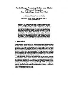
original algorithm took about 90 minutes on a single 450MHz Pentium III CPU to compose 123 images into a single mosaic. This algorithm change reduces the required CPU time to about 48 minutes. Running the same algorithm and problem on an 800MHz CPU reduces the time to about 28 minutes (Figure 1b). To exploit the parallelism available on a cluster, the parallel mosaic algorithm divides the targeted mosaic into N slices, where N is the number of CPUs (N=4 in Figure 1a as indicated by horizontal lines). Once each CPU has completed its tasks, it reports the image slice to the manager CPU, which then patches the slices together into one image and saves it to disk. Results of the parallelization of the mosaic algorithm are shown for the 800MHz cluster and for the 450MHz cluster in Figure 1b. The dot-dashed line shows the ideal speed-up. The actual timings follow a linear scaling with deviations from the ideal attributed to load balancing problems and data staging problems. The 800 MHz curve extends to a larger number of CPUs since our 800 MHz cluster has twice as many CPUs available. Detailed issues on load balancing and data staging are discussed in references [4,5].
4. Parallel stereo image correlation 4.1. Overview and primary results
Figure 1: (a) Mosaic generation from individual image frames. The horizontal lines in the panorama indicate the strips of the image that are distributed to different CPUs i n the cluster. The images were taken from a FIDO Rover field test in the beginning of May, 2001. (b) Timing for the assembly of 123 individual images into a single mosaic for two different clusters.
Two eyes in humans provide depth perception. The images are obtained from two independent optical systems, the brain correlates the two, and provides a 3-D impression. The same principle is utilized with stereo image cameras. The Mars Exploration Rovers carry several cameras including two dedicated sets of stereo camera pairs for navigation, hazard avoidance and science. The stereo images are used to determine distances to certain objects and to generate 3-D terrain maps. While the optical correlation in the brain appears to function with incredible ease, the digital correlation of two images is a numerically intensive task. The original algorithm used for Mars stereo image correlation was developed [2] in the Multi-mission Image Processing Laboratory (MIPL) over several decades. The original algorithm consumed typically 90 minutes on a 450MHz Pentium III CPU. Under some conditions the algorithm was plagued by convergence problems, which could result in computation times of days or longer. The new parallel algorithm partitions the reference image into separate segments that are processed on different CPUs. The correlation target is available to all CPUs and no segmenting is performed (see Figure 2). The new algorithm requires about 55 minutes on a single 450 MHz CPU (due to algorithm changes) and requires about 4.5 minutes on 16 CPUs. Running the same problem on an 800MHz Pentium III cluster reduces the time further to about 3 minutes on 16 CPUs. Tests on inputs that choked the original algorithm with convergence problems showed that the new algorithm appears to be no longer subject to these pathologies.
36
30
24
18
12
6
35
29
23
17
11
5
34
28
22
16
10
4
33
27
21
15
9
3
32
26
20
14
8
2
31
25
19
13
7
1
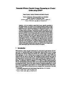
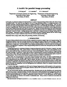
Figure 2: Left and right image of a rover camera. The left (reference) image is subdivided into segments that are correlated independently to the right target image by independent CPUs. The left image has a blue shade overlaid to indicate the pixels that have been found by a left=>right correlation. Note that patch 34 indicates an erroneous correlation since that part of the image is not even in the right image.
4.3. Elements of the correlation algorithm The numerical correlation algorithm tries to find for every pixel in the left image a corresponding pixel in the right image. The algorithm starts from a pre-defined seed point defining a pixel in the left image, and attempts to correlate this pixel and a set of surrounding pixels with those in the right image. A camera model that gives information relating the geometry of the two cameras is used to find the starting location in the right image given a pixel in the left image. Starting at the seed point, the correlation process spirals outward until new pixels can no longer be correlated with each other. The algorithm then begins anew with a different seed point and continues attempting to correlate pixels that have not been previously processed. In between the main correlation stages, a pass is made along the areas not previously correlated to complete the correlation in those sections of the image pair. This stage is referred to as filling the gores in the image. Generally not all pixels can be correlated, due to the different view angles of the two cameras. For example in Figure 2 the left eye sees an area of ground between the lower ramp and the left of the rover that the right eye does not see at all (segment 13 in Figure 2). Also the complete first column (segments 3136) is not present in the right image.
4.3. Parallel image correlation algorithm Before the existing algorithm was parallelized, a timing analysis was performed in order to determine in which functions most of the time is spent. Most of the time is indeed spent in the core function that performs the actual correlation evaluation of a few pixels (as opposed to set-up functions or the drivers that feed pixel pairs to the core correlator). However the analysis showed that the
algorithm was called several orders of magnitude more often than there are pixels to correlate. Most of the calls resulted in an immediate return since the particular pixel pair had been correlated already. Such a multi-level testonly entry and exit from a function is computationally very expensive since it results in register push operations. We moved this check outside the function call to remove this inefficiency. We also reduced the overall number of correlation existence checks by several algorithm changes. One of the major contributors to failed correlations is the attempt to correlate edge pixels that only exist in the left image but not in the right. These algorithmic changes resulted in a reduction of required CPU time by about 1020%. After initial algorithm improvements and an analysis of actual times spent in the core correlation function we could determine an appropriate path for program parallelization. Individual calls to the core correlation function consume about 0.5ms (on an 800MHz Pentium III). The actual execution time of this function call depends on correlation input; i.e. the correlation of an initial seed point, the correlation on a window edge and the correlation of remaining gores take different times. Fine grain parallelization of this function call would be completely futile for such a fast execution time because communication costs such as sending a message to another CPU or sharing information between threads will cost about that much time (within a factor of 10). We therefore decided to divide the image into segments and perform the correlation of the segments independently on different CPUs (as indicated with the grid in Figure 2). A division of the image into several independent segments is a significant deviation from the original algorithm, which was based on the correlation on the edge of an ever-increasing window. Segmenting the image results in the introduction of new borders across which correlation cannot proceed [6]. The different segments can be separated by an arbitrary number of bits as designated
parameter to check the influence on the total compute time. This influence is shown to be weak. Time (Minutes on log scale)
by user input. Parallel correlation will be only performed with a segment. The correlation gaps between different segments can be filled in by a subsequent single CPU correlation of the overall image size. Possible transitions between different segments can therefore be smoothed out. In the example cases we studied it appeared that there were no problems at the edges of the different correlation domains and the second pass with a single CPU run was not necessary. The separating frame width between CPU segments is therefore set to zero by default. Another algorithm change that was necessary before the program could be parallelized was the implementation of a seed generation algorithm that can be called on an arbitrary segment of the image. The original algorithm fed a list of seed points distributed evenly throughout the image, yet uncorrelated or random to the image data. Within the newly implemented seed generation algorithm we pick the first point in the dead center of the segment. Sub-sequent points are picked at random within the segment. If the new seed pixel has been correlated already or if the quality of a seed (as evaluated by a single pass through the correlator) is insufficient, a new seed is generated. After a seed is generated the algorithm remains the same within an image segment. Since the correlation of seed points, window edges and gores can take a different time one can easily imagine that different CPUs working on the different image segments may finish at different times. To prevent the run-away correlation delay of a single CPU that will hold up all others (as experienced in the original single CPU code) we limit the number of times correlations are attempted. The correlation within the segments on the different CPUs is controlled by a maximum number of (successful) seed generations and a desired filling percentage of correlated pixels. The correlation is stopped once the maximum number of trials has been executed or if the desired filling percentage has been achieved. A time-based cut-off that synchronizes all CPUs against a desired maximum execution time as well as a master-slave approach to even out the work load have been considered but were not implemented. With the algorithm changes described above we have tested image pairs that caused the original correlation algorithm to run for weeks at a time. Our new algorithm does not suffer from this pathology any more and finishes with average time comparable to other image pairs. The number of correlated points was approximately the same as any other image pair (80-90%). The successful finish of the new algorithm is not due to a premature stop of the correlation, which might leave one segment completely uncorrelated. We believe that the original code was stuck on gore point correlations due to bad seeds. The segmentation of the image speeds up the search for the remaining gores and their processing significantly. Figure 3 shows the reduction of processing time with increasing number of CPUs for two different image sets. The scaling is found to be almost perfect for up to 50 CPUs. The number of maximum seed trials is used as a
Image Set 1
36
Image Set 2 1 seed 10 seeds 20 seeds
1 seed 10 seeds 20 seeds
10
Serial
Serial 4 3 2 1 time ideal 1
50 1 10 20 # of CPUs on log scale
time ideal 20 50 10 # of CPUs on log scale
Figure 3: Correlation time as a function of utilized CPUs o n an 800MHz PIII cluster for two different image sets and a different number of trial seeds. (the actual image set 2 is not shown here).
5. Correlation quality measurements 5.1. Introduction The parallel correlation algorithm has been significantly modified from the serial algorithm in terms of the handling of the seeds and the areas in which correlation is performed. The natural question that arises now is how good are the correlations generated with the new algorithm compared to the old algorithm? Visual inspection of the correlation data seemed to indicate an acceptable performance, but no quantitative measurement algorithm was available. A direct comparison between the serial and parallel output showed excellent agreement in large areas, but significant disagreement in some smaller areas. Noting that the serial code also might generate erroneous correlation data as indicated above, we developed a quantitative quality assessment algorithm.
5.2. Correlation quality algorithm The stereo image correlation software attempts to deliver for every pixel (x, y) in the reference image (left) a corresponding pixel coordinate (x', y’) in the corresponding pair (right) (Fig. 4a). A simple test to assess the quality of the left=>right correlation is to check if a right=>left correlation can return the originating point. The basic principle is depicted in Fig. 4b). It is based on establishing TWO correlation maps left=>right and right=>left, therefore doubling the overall workload. The originally desired mapping relates the red point (x,y) to the green point. The corresponding mapping from the green point back to the left will result in the orange pixel (x'',y''). A mapping is considered perfect if (x,y) and (x'',y'') are identical. The very strict criterion of a perfect match can be relaxed by the introduction of an error window (indicated by the yellow square), which accounts for integer interpolation round-off and a small amount of noise. The influence of this error window size as a
measure of correlation quality will be explored further (a)
(x,y)
left image (b)
(x,y)
(x',y')
l->r
right image l->r
(x',y')
(x'',y'')
left image (c)
(x,y) (x'',y'')
left image
right image l->r l->r
(x',y') r->l (x''',y''') right image
Figure 4: (a) correlation mapping from left to right. (b) l=>r and r=>l mapping with an acceptable error window. (c) Closed-loop checking with error windows in the left and right correlation.
nav_edr_20000509155356_l.img,orig_lr2.mask
12 3 4 567 8 nav_edr_20000509155356_l.img,out_lr_n16_s10_2.mask
below. The correlation verification laid out in Fig. 4b) relies on the quality of the right=>left correlation, which in itself is questionable. If a finite error window size is considered a situation may arise as depicted in Fig. 4c), where the l=>r and r=>l verification starting from (x,y) works out fine (red=>green=>orange), however, the r=>l and l=>r verification starting from pixel (x',y') does not (green=>orange=>blue). If such a deviation occurs we should have not accepted the mapping from the green dot to the orange dot in the first verification starting at the red dot. Our algorithm has the option to filter out such cases by running the pair of algorithms repeatedly with the output of the first pass as an input the new pass. At each step a correlation pair that has resulted in a bad correlation connection is thrown out of the list of available pairs. This algorithm is repeated until no bad correlation pairs are found anymore. This way the filtering does bear some sense of self-consistency in it.
5.3. Parallel. vs. serial code validation The top row of Fig. 5 shows the left and right images
nav_edr_20000509155356_r.img,orig_lr2_12.mask
12 3 4 5 67 8 9 nav_edr_20000509155356_r.img,out_lr_n16_s10_2_12.mask
Figure 5: left/right images (yellow) overlaid with the validated correlation mask (blue) for the serial (top) and parallel (bottom) algorithm. The quality check eliminates the previously the bad correlation data (red lines). The parallel algorithm finds more correlated regions than the serial algorithm (green lines). However the correlation of a checkerboard problem i s still not eliminated (yellow lines).
nav_edr_20010429172202_l.img,out_lr_n16_s10_2.mask
nav_edr_20010429172202_r.img,out_lr_n16_s10_2_12.mask
Figure 6: Image set 2 (yellow) overlaid with verified correlation mask (blue) generated in parallel on 16 CPUs with 1 pixel acceptable deviation. 220k
raw / unchecked pixels Image Set 1
200k Number of Pixels
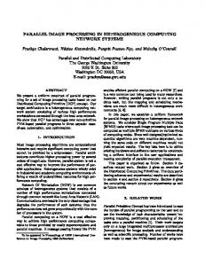
overlaid with the verified correlation masks of the original serial correlation algorithm. The allowed pixel deviation is 1. The area that was wrongly correlated in the left image has been eliminated by the quality control algorithm (see large rectangle on the top left of Figure 5 – corresponding roughly to the frame numbered 34 in Figure 2). The second image row of Figure 4 corresponds to the results from the parallel code run on 16 CPUs (with 10 maximum seed iterations) after a quality check with the algorithm above (accepted pixel deviation 1). The parallel code does find areas of correlations that the serial code did not explore at all, due to the subdivision of the image (big green rectangle). Some patterns are recognized on the rover correctly (small green rectangle) but other regions are not (small yellow rectangle). Figure 6 depicts the second image set with an overlaid correlation mask that was obtained with 16 CPUs and verified with 1 pixel acceptable deviation. Figure 7 depicts the number of pixels returned from the correlation algorithms as a function of number of CPUs used in the parallel algorithm for image set 1 and 2. There are 4 different quantities depicted: 1) the raw/uncorrected pixels (largest number), 2) the corrected pixels allowing for 0 pixel deviation during the mapping correction (smallest number), 3) corrected pixels with allowed error of 1 pixel, and 4) allowed error of 2 pixel. The 0 pixel error requirement is very strict, especially since there can be simple pixel round-off errors leading to the elimination of a good pixel pair. Allowing for a 1 pixel deviation increases the number of acceptable pixels by about 10%. There is not a large difference in number of corrected pixels allowing for 1 or 2 pixel errors. The graph also shows that hitting the correlation algorithm with 20 over the standard 10 maximum seed points increases the number of raw pixels but not the number of good pixels. The dependence of the number of
Serial 10 Seeds 20 Seeds 2 pixel dev.
160k
120k 100k 0
Image Set 2
raw / unchecked pixels
240k
180k
140k
250k
230k checked: 2 pixel deviation
checked: 2 pixel deviation
220k
checked: 1 pixel deviation
210k
checked: 0 pixel deviation
10
20 30 # of CPUs
40
50
200k 0
checked: 1 pixel deviation Serial 10 Seeds 20 Seeds 2 pixel dev.
checked: 0 pixel deviation
10
20 30 # of CPUs
40
50
Figure 7: Number of pixels correlated for two different image sets as a function of number of CPUs used in the parallel algorithm with the allowed pixel deviation as a parameter. The serial results are indicated at 1 CPU with a solid red dot. The dependence of the quality of correlated pixels on the number of CPUs in the parallel algorithm i s weak. Also the dependence on the maximum number of seeds (10 / 20) is weak. Allowing for 1 pixels deviation increases the number of acceptable pixels by about 10%. Increasing the allowed error window to 2 pixels does not add many more acceptable correlation points.
(successfully) correlated pixels on the number of CPUs used in the parallel algorithm is weak. Image set 1 (Figure 5) clearly does not correlate well at all. These sets contain a lot of sharp edges of the rover and the ramp that the correlation parameters are apparently not well tuned for. The correlation algorithm returns significantly more verified correlation points for image set 2 (Figure 6).
5.4. Validation of simplified algorithms The correlation algorithm has several lower level correlation modes available to the user. The algorithm historically used most of the time is the so-called Amoeba algorithm. It performs a correlation matrix evaluation in a six dimensional space that allows for image displacement, resizing, and rotation. The
Table 1: Comparison of image correlation quality for two different images and two different correlation algorithms. Image1 Image1 Image2 Image2 Mode Amoeba Amoeba2 Amoeba Amoeba 2 Time 145.3 22.523 149.5 22.9 6.4 x 6.5 x Total 307200 307200 307200 307200 Pixels Good 136314 134747 227774 217400 Pixels 44.4% 43.9% 74.1% 70.8% Bad Pixels 170886 172453 79426 89800 55.6% 56.1% 25.9% 29.2% Pixels in N/A 161108 N/A 77678 Neither Pixels in N/A 11345 N/A 12122 Ref. Only Pixels in N/A 9778 N/A 1748 mode only 7.3% 0.8% Line 0 Pix. N/A 122841 N/A 214422 Deviation 91.2% 98.6% Line 1 Pix N/A 1926 N/A 1197 Deviation 1.4% 0.6% Line 2 Pix N/A 125 N/A 31 Deviation 0.09% 0.01% Line>2Pix N/A 77 N/A 2 Deviation 0.06% 2 N/A 93 N/A 38 Pix. Dev. 0.6% right and right=>left image correlation. The correlation quality algorithm can also be used to test various correlation algorithms against each other. The parallel software developed in the research-oriented Applied Cluster Computing Technologies group was delivered to the MIPL team and integrated into the MIPL operational system.
7. Acknowledgements This research was carried out by the Jet Propulsion Laboratory, California Institute of Technology under a contract with the National Aeronautics and Space Administration. The work was sponsored by the TMOD technology program under the Beowulf Application and Networking Environment (BANE) task and by the ESTO CT program. The original VICAR based software and the new parallel versions are maintained in the Multi-mission Image Processing Laboratory (MIPL) [2,7].
8. References [1] Michael S. Warren, John K. Salmon, Donald J. Becker, M. Patrick Goda, Thomas Sterling, Gregoire S. Winckelmans, Pentium Pro Inside: I. A Treecode at 430 Gigaflops on ASCI Red, II. Price/Performance of $50/Mflop on Loki and Hyglac, SC97 Conference Proceedings, 1997. [2] Multi-mission Image Processing Laboratory http://www-mipl.jpl.nasa.gov [3] Tom Cwik, Gerhard Klimeck, Myche McAuley, Charles Norton, Thomas Sterling, Frank Villegas and Ping Wang, The Use Of Cluster Computer Systems For NASA/JPL Applications, AIAA Space 2001 Conference and Exposition, Albuquerque, New Mexico, 28 - 30 Aug 2001.
[4] Tom Cwik, Gerhard Klimeck, Myche McAuley, Bob Deen and Eric Dejong, "Applications on High Performance Cluster Computers Production of Mars Panoramic Mosaic Images", Proceedings of the 2001 AMOS Technical Conference, September 10-14, 2001, Maui [5] Parallel Mars image processing web http://hpc.jpl.nasa.gov/PEP/gekco/mars
site:
[6] We decided for the first parallelization attempt to not transmit correlation information of adjacent segments to
adjacent CPUs, which is associated with significantly increased communication and algorithm complexity costs. [7] Susan K. LaVoi, William B. Green, Allan J. Runkle, Douglas A. Alexander, Paul Andres, Eric. M. DeJong, Elizabeth D. Duxbury, David D. Freda, Zareh Gorjian, Jeffrey R. Hall, Frank R. Harman, Steven R. LaVoi, Jean J. Lorre, James M. McAuley, Shigeru Suzuki, Pamela J. Woncik, John R. Wright, Processing and analysis of Mars Pathfinder science data at the Jet Propulsion Laboratory’s Science Data Processing Systems Section. J. Geophys. Res. Vol. 104, No. E4, p. 8831 (1999).