Nearest Manifold Approach for Face Recognition Junping Zhang Intelligent Information Processing Laboratory Fudan University, Shanghai, China
[email protected]
Stan Z. Li Microsoft Research Asia Beijing, China
[email protected]
Jue Wang Institute of Automation, Chinese Academy of Sciences Beijing, China
[email protected]
Abstract Faces under varying illumination, pose and non-rigid deformation are empirically thought of as a highly nonlinear manifold in the observation space. How to discover intrinsic low-dimensional manifold is important to characterize meaningful face distributions and classify them using a simpler, such as linear or Gaussian based, classifier. In this paper, we present a manifold learning algorithm (MLA) for learning a mapping from highly-dimensional manifold into the intrinsic low-dimensional linear manifold. We also propose the nearest manifold (NM) criterion for the classification and present an algorithm for computing the distance from the sample to be classified to the nearest face manifolds in light of local linearity of manifold. Based on these works, face recognition is achieved with the combination of MLA and NM. Experiments on several face databases show that the advantages of our proposed combinational approach.
1 Introduction Face recognition system from images is of particular interest to researchers owing to its wide scope of potential applications such as identity authentication, access control and surveillance. It is a quite challenging task to develop a computational model for face recognition because faces are complex, multidimensional, and meaningful visual stimuli [15]. Much research on face recognition, both by computer vision scientists and psychologists [10], has been done over the last decade. From the aspect of computer vision, face recognition can be roughly distinguished into two categories: geometric feature-based approaches and template matching approaches. In the first category, facial feature values depend on the
detection of geometric facial features like eye corners and nostril[17][4]. However, the first one is time-consuming and complex about modeling face. The second one assumes that an image as single or multiple arrays of pixel values[19]. The virtue of template methods is that it is not necessary to create representations or models for objects. Most recognition systems using linear method are bound to ignore subtleties of manifolds such as concavities and protrusions, and this is a bottleneck for achieving highly accurate recognition. This problem has to be solved before we can make a high performance recognition system. Generally speaking, faces are empirically thought to be constitute a highly nonlinear manifold in the observation space[7][12]. We therefore assume that an effective face recognition system should be based on ”face manifold”, and the full variations in lighting condition, expression, orientation, etc. may be viewed as intrinsic variables which generate nonlinear face manifold in observation space. Currently, rich literature on how to learn nonlinear manifold has grown up and can be roughly divided into four major classes: projection methods, generative methods, embedding methods, and mutual information methods. 1. The first one is to find principal surfaces passing through the middle of data, such as the principal curves [5]. Though geometrically intuitive, the first one has difficulty on how to generalize itself into higherdimensional manifold. 2. The second one such as generative topology model [2], hypothesizes that observed data are generated from the evenly spaced low-dimensional latent nodes. Nevertheless, the generative models fall into local minimum easily and have slow convergence rates. 3. The third one is generally divided into global and local embedding algorithms. Global ones like Isometric
Mapping (henceforth ISOMAP) [14] presume that in affine sense, isometric properties should be preserved in both the observation space and the intrinsic embedding space, while local ones like Locally Linear Embedding (LLE) algorithm [9] and Laplacian Eigenamp approach [1] focus on the preservation of local neighbor structure.
is a linearly weighted average of its neighbors, is thought of as initialization of our proposed MLA to extract the underlying feature of face data. Let the training set of face in the observation space be C (where C ∈ RN , N À d), the corresponding intrinsic low-dimensional set Z (Z ∈ Rd ) is obtained with LLE algorithm. The details of LLE algorithm can be referred as to [9]. And then the completed set (C, Z) is used for the subsequently modeling of the mapping relationship of the manifold. A disadvantage of LLE algorithm is that the mapping of test samples is difficult for the computational cost of eigenmatrix. Thus, we propose an alternative manifold learning model based on the completed data set (C, Z), where Z is the corresponding low-dimensional mapping result of training data C. Mathematically, a smooth manifold can be alternatively represented by a set of local coordinate systems or atlas {(Uα , φα ), α ∈ A}, where A is the index set. Each chart of atlas reflects a local linear mapping property of manifold. To avoid the difficulty of choosing a special chart, kernel method is used for obtaining the metric property of the chart from the original space without an explicit understanding of the mapped chart [16]. Suppose that the mapping function {φ} of each chart is orthogonal basis of hilbert space H, then the mapping function {φ} is defined as follows:
4. In the fourth category, it is assumed that the mutual information is a measurement of the differences of probability distribution between the observed space and the embedded space, as in stochastic nearest neighborhood (henceforth SNE) [6] and manifold charting [3]. While there are many impressive results about how to mine the intrinsic invariants of face manifold, manifold learning on face recognition has fewer reports. A possible explanation is that the practical face data include a large number of intrinsic invariant and have high curvature both in the observation space and in the embedded space, and meanwhile the effectiveness of currently manifold learning methods strongly depend on the selection of neighbor parameters. To address the problem, we present MLA for recovering the intrinsic low-dimensional space embedded face manifold in the observation space in section 2. And then we propose NM approach to distinguish face manifold with the computation of the nearest manifold distance from sample to be classified to face manifold in section 3. With the combination of MLA and NM, experiments carried out on several face databases show that advantages of our proposed method in section 4.
2
−Ci2
φ(Ci ) = e
√
r
(1, 2Ci , · · · ,
1 √ ( 2Ci )n , · · · ) n! Ci ∈ C
(1)
With the Taylor expansion, the metric from sample to some chart is represented as follows: k(Ci , xj )
Manifold Learning Algorithm
= φ(Ci )φ(xj ) = e−kCi −xj k
There are generally high curvature regions on the manifold of an face in the image space, when the face is subject to various changes. Such nonlinearity is one of the main reasons that impairs recognition performance. A trade-off method is to unravel the low-dimensional linear space of image manifold with some dimensionality reduction methods. Recently, manifold learning provides an interesting way to discover the intrinsic dimensionality of image manifold. However, most of manifold learning methods lack an effective way to model relationship from face manifold into low-dimensional space without dimensionality limitation and also have fewer applications on face recognition. We therefore propose different MLA to model mapping relationship between low-dimensional embedded space and face manifolds in the observation space to address the problem. First, LLE algorithm, which presumes that each sample both in the observation space and in the embedded space
2
(2)
It is easy to find kφ(x)k = 1. Consequently, we obtain the metric property of each chart by the adoption of kernel method. Consider the length of paper, we delay the proof in the future paper. In reality, we select Gaussian RBF kernel function which is a variant of Formula (2) as follows: k(Ci , xj ) = exp(− k Ci − xj k2 /2σ 2 )
(3)
where parameter σ 2 can be predefined or computed with respect of data distribution. To analysis the global structure of manifold however, it is necessary to unite these charts into a uniform coordinate system. A simple strategy is that global coordinates of intrinsic low-dimensional manifold be obtained by the weighted factor multiplied the similarity metric of data in each local coordinate system. If each training sample is thought of as origin of a chart, the mapping relationship of 2
4
dataset (X, Y ) is modeled in light of formula (4) as follows: yj =
m X
3
d
αi k(Ci , xj ), Ci ∈ C; xj ∈ X; yj ∈ R
(4)
2
i=1 1
where Y = {y1 , . . . , yn } ∈ Rd , X = {x1 , . . . , xn } ∈ RN , m as the number of training samples, A = {ai } the d × m weighted mapping matrix. As a matter of fact, we also model the inverse mapping relationship from the intrinsic low-dimensional space into the observation space with the same idea. Consider the completed data set (C, Z), the mapping weighted matrix A is formulated as follows: A = Z · (k(Ci , Cj ))−1 , i, j = 1, . . . , m
0
−1
−2 −4
−3
−2
−1
0
1
2
Figure 1: 1956 examples mapped to the 2-D MLA subspace .
(5)
Actually, introducing some regularization terms or pseudo-inverse is necessary to prevent the degeneration of the inverse kernel matrix in Formula (5). Given the weighted mapping matrix A, training data set C and the parameter σ 2 of kernel matrix, the corresponding lowerdimensional mapping result of test sample is then computed as follows: ξ=
m X
αi k(Ci , η), αi ∈ A; η ∈ RN ; ξ ∈ Rd
(6) Figure 2: The corresponding reconstruct faces
i=1
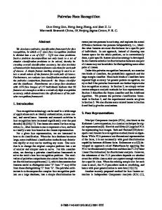
where η is a test sample in the observation space, and ξ the corresponding low-dimensional mapping point. Consequently, the mapping relationship from the observation space into the embedding space is modeled with our proposed MLA. It is apparent that we may also reconstruct the corresponding data in the observation space for unknown lowdimensional sample in similar way. By calculating Formula (6), the nonlinear mapping model between face manifold in the observation space and the corresponding lowdimensional space is established and therefore the intrinsic low-dimensional linear space of is approximately recovered. In this paper, the Frey face database (20*28 pixels, 1956 examples) [9] is used to explain our proposed MLA method. Firstly, in the MLA learning stage, the 491 cluster centers are extracted using vector quantization and mapped into 2D space using LLE. Then all the 1956 face examples are mapped into the 2-D space based on the mapping learned in the first stage where σ 2 = 100, as shown in Figure 1. Thirdly, we randomly sample two points and use them as the upper-left and lower-right corner points for a rectangle, and then sample 11 evenly spaced points along each of the boundary and diagonal lines of the rectangle, and these points are reconstructed with MLA, as displayed in Figure 2. We observe that a continuous expressional change in the vertical axes and pose change from the right side to
the left side. Therefore, we have approximately recovered 2 intrinsic principal features, those of expression and pose, for the FREY database using our proposed method.
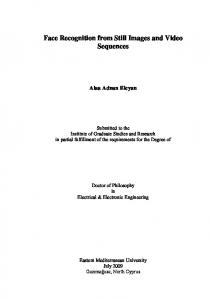
3 Nearest Manifold Approach While MLA is capable of extracting some intrinsic invariants from face manifold, it is yet difficult to recognize face from different face manifolds. A possible explanation is that current techniques on manifold learning are ineffective to recover the intrinsical low-dimensional linear space accurately. However, we hypothesize that local linearity of low-dimensional space obtained through MLA is better than that of face data in the observation space. With this assumption, NM approach, which is a generalization of the NFL method [13], are adopted for face recognition under the lowdimensional space obtained by MLA. It calculates the local projection distances from sample to be classified to each local Euclidean space and then recognizes face through learning globally nearest manifold distance with respect to local projection distances. The basic idea of NM approach in three-dimensional space is illustrated as Figure 3. In the figure, the triangle ∆T1 T2 T3 represents a local linear hyperplane of face manifold. By extending the three edges of the triangle to 3
Triangle Vextex Extended Vertex Projection Point Tested Sample Edge of Triangle Extended Line Projection Line Pseudo−Projection Line
1.4
y1
1.2
E6
The other two projection indices remain the same computation as in Formula (8). We define the six vertex polytopy by constraining the weights λ to be in the range of [−γ, 1 + γ]. In case 2, some of them are in the range [−γ, 0] ∪ [1, 1 + γ] (In our experiments, the parameter γ is set value 0.5 manually without loss of generality), the corresponding three projection points from sample to the three edges of the triangle ∆ are then computed as follows: T1 + λi (T1 − T3 ), i = 1 T2 + λi (T2 − T3 ), i = 2 Pi = (10) T1 + λi (T1 − T2 ), i = 3
1
E5
0.8
T3
0.6
E1
0.4
P1
0.2 0
y3
T1 E2
T2
−0.2
E4
−0.4 2
P2
P3 P4
1.5
E3
1.5
y2
1
1 0.5
0.5
0 0
−0.5
Figure 3: The Basic Idea of NM approach
Where P 1 , P 2 and P 3 denote the projection indices from sample to edge T1 T3 , T2 T3 and T1 T2 , respectively. Thus, the projection distance from sample to local hyperplane is defined as follows:
vertices E1 to E6 , we obtain an extended local hyperplane (see discussion below for the scope of the extension). For the explanation of NM approach, furthermore, test samples from y1 to y3 , and the corresponding projection points of test samples from P1 to P3 are also shown in the figure. Three cases are considered in the computation of the nearest projection distance according to NM approach:
d(y, P i ) = min ky − P i k, i = 1, 2, 3 i
In case 3, the sample is projected outside the extended polytope, and all the weights are in the range (−∞, −γ) ∪ (1 + γ, ∞). Consider locally linearity of low-dimensional space with MLA, it is inaccurate to compute the projection index with respect to Formula (7) or Formula (10), a simple way is to calculate the distance from sample to nearest extended vertex. For example, the projection point P3 of sample y3 is equal to the extended vertex E4 as in Figure 3. After defining the locally nearest manifold distance dN T (yi , ∆j |Mk ) given the sample yi , the triangle ∆j of image manifold Mk , it is not difficult to calculate the local projection distances from sample to all the triangles of manifold iteratively. Once the overall computations of local projection distances on the same manifold are completed, the globally nearest manifold distance from sample yi to manifold Mk is calculated as follows:
1. The sample y is orthogonally projected into the inner of the triangle ∆T1 T2 T3 . For example, y1 is projected as point P1 in Figure 3. 2. The sample y is orthogonally projected outside the inner of the triangle but within the polytope formed by the six extended vertices E1 to E6 . For example, y2 is projected as point P2 in Figure 3. 3. The sample y is orthogonally projected outside the polytope formed by the six extended vertices E1 to E6 . For example, y3 is projected as point point P4 in Figure 3. For case 1, given the k-th locally linear manifold Mk , the projection point P of sample y is computed as follows: P =
3 X
dN M (yi |Mk ) = d
λi Ti , Ti ∈ Mk ; Mk ∈ R ; k = 1, · · · , K (7)
where the weights λi of each vertex of triangle are calculated as follows: ½ (AT A)−1 AT (y − T3 ), i = 1, 2 λi = (8) 1 − λ1 − λ2 , i=3
dN T (yi , ∆j |Mk ) (12)
where mk is the number of training samples of the k-th face manifold, ∆j is the j-th constrained nearest triangle, Mk means the k-th face manifold. It is not too difficult to know that total number of triangle of each face manifold data Pthe mk 2 . When the parameter mk is equal to 2, nearis l=3 Cl−2 est projection distances of NM approach are computed with respect to Formula (10). When the parameter mk is equal to 1, the nearest neighbor algorithm is used for the computation of nearest manifold distance. The nearest manifold classification is formulated as follows:
A = [T1 − T3 T2 − T3 ], y ∈ Rd
In this case, the weights satisfy 0 ≤ λi ≤ 1. For cases 2 and 3, the weights λ3 is re-calculated and represents the projection index from sample to edge T1 T2 as in Formula λ3 = (T1 − T2 )T (y − T2 )/kT1 − T2 k
min Pm k 2 j=1,..., l=3 Cl−1
i = 1, . . . , n; k = 1, . . . , K
i=1
where
(11)
C(yi ) = arg min dN M (yi |Mk )
(9)
k
4
(13)
where C(yi ) represents which classes sample yi belongs to, K is the number of different face manifolds. Though our illustration of nearest manifold approach is completed under the 3-dimensional space, the proposed nearest manifold approach can be generalized to arbitrarily higher dimensional space. TheP total computational complexity of NM approach mk 2 is O(K × l=3 Cl−1 ).
Table 1: Error rates MLA+NM 3.73% 3.83% 2.99% 12.39%
UMIST(150) ORL(120) JAFFE (50) EXPRESS(150)
4 Experiments
MLA+NN 5.71% 7.75% 8.86% 13.73%
PCA+NM 4.83% 8.13% 8.76% 16.63%
PCA+NN 8.11% 9.86% 11.12% 32.94%
In our experiments, two parameters (neighbor factor K 0 of LLE algorithm and σ 2 of kernel function) need to be predefined for MLA. Without loss of generality, we set K 0 be 40 for ORL, UMIST and Jaffe expression database, 20 for JAFFE Face database, and set σ 2 be 10000 for ORL and UMIST databases, 8000 for JAFFE expression and face database.
Experiments are carried out to evaluate the performance of the proposed MLA and NM methods in face recognition performance using three face databases, namely the Olivetti (ORL) [11], UMIST [18] and JAFFE [8] databases. The ORL database consists of 10 different images for 40 people each (four female and 36 male subjects). The UMIST database consists of 575 images of 20 people with varied poses (-90 degree to 0 degree).And We crop images into 112*92=10304 pixels. The JAFFE database, which has been used in facial expression recognition, consists of 213 images of 10 Japanese females. The head is almost in frontal pose. The number of each image represent one of the 7 categories of expressions (neutral, happiness, sadness, surprise, anger, disgust and fear). In our experiment, the database is used for both oriental face recognition and expression recognition. All these images of JAFFE database are cropped to the size of 146 × 111 pixels. For ORL database, the 10 images of each of the 40 persons are randomly partitioned into two sets, namely, 200 training images and 200 test images, without overlapping. As for dimensionality reduction, the biggest reduction dimensions of the training set are first set to be 120. And then the reduction dimensions is gradually decreased according to the descending order of eigenvalues LLE algorithm used. As for UMIST database,10 images of each person are randomly selected as the training set, and the remaining 375 images as the test set. The JAFFE database is partitioned into two sets: 6 images of each of the 10 persons are randomly extracted to make 60 training set and the remaining 153 images are used as the test images. Meanwhile, in expression recognition, 24 images of each expressional categories are randomly extracted to make 168 training set and the remaining 45 images are used as the test set. In order to compare the performance of MLA and NM approach, we introduce a classical linear dimensionality reduction algorithm – PCA [15], and then design four combinational algorithms: the combination of 1-nearest neighborhood with PCA (PCA+NN), the combination of NM with the PCA (PCA+NM), the combination of 1-nearest neighborhood with MLA (MLA+NN), the combination of NM with MLA (MLA+NM).
0.2
0.2
0.18
0.16
0.16
0.14
0.14
0.12
0.12
Error Rates
Error Rates
MLA+NN MLA+NM PCA+NN PCA+NM
ORL Face Recognition
0.18
0.1
0.1
0.08
0.08
0.06
0.06
0.04
0.04
0.02
0.02
0 10
0
20
30
40
50
60
70
80
Number of Dimension
90
100
110
120
40
60
80
100
120
140
(b) UMIST Face Recognition
0.2
0.5
MLA+NN MLA+NM PCA+NN PCA+NM
JAFFE Face Recognition
0.18
0.16
0.4
0.14
0.35
0.12
0.1
0.08
0.06
MLA+NN MLA+NM PCA+NN PCA+NM
JAFFE Express Recognitoin
0.45
Error Rates
Error Rates
20
Number of Dimension
(a) ORL Face Recognition
0.3
0.25
0.2
0.15
0.04
0.1
0.02
0.05
0 10
MLA+NN MLA+NM PCA+NN PCA+NM
UMIST Face Recognition
15
20
25
30
35
40
45
Number of Dimension
(c) JAFFE Face Recognition
50
0 20
40
60
80
100
120
140
Number of Dimension
(d) JAFFE Express Recognition
Figure 4: Recognition Comparison All the experimental data have been normalized. And the experimental results are the average of 100 repetitions. The results are illustrated as in Figure 4(a), Figure 4(b), Figure 4(c), and Figure 4(d), respectively. The Error rates (ER) of face recognition in the biggest reduced dimensions as in Figure 4 are tabulated in Table 1. It can be seen from the figures and table that the MLA+NM algorithm than the other three combinational algorithms has better recognition result. For example, in Table 1, the error rates of MLA+NM algorithm is about 46% of the PCA+NN, 77.2% of the PCA+NM, and 65.3% of the 5
MLA+NN on the UMIST face database. In Figure 4(a) and Figure 4(b), error rate based on MLA+NM than on PCA+NM need higher reduced dimensions to reach stability when the reduction dimensionality is 90 dimensions or so. We presume that manifold learning methods than PCA methods can extract more intrinsic features of face manifolds. With MLA+NM, both the recognition ability and the stability of error rates have remarkable improvements. We assume that the ability of the MLA recovering the intrinsic linear embedded space is approximate and even locally linear, and then NM approach improves the recognition performance through the computation of global nearest manifold distance with local projection technique. It is worthy noting that several parameters affect final experimental results. For example, the influences of variance σ 2 and training samples on UMIST face recognition are illustrated as in Figure 5(a) and Figure 5(b), respectively.
show the advantages of our proposed methods. With the combination of MLA and NM, a relatively effective recognition system is constructed. MLA is first used for recovering the intrinsic low-dimensional space of face manifolds. And then NM is used for identifying face through searching the nearest manifold distance. Results with the JAFFE database show that we achieve effective recognition of the two different cognitive concepts (face and expression recognition) only by applying the same manifold learning mechanism. The interesting results may lead to broader applications which will be studied in future work. Also we will compare the proposed manifold learning methods with the state-of-the-art algorithms on large-scale face database such as FERET.
References [1] Mikhail Belkin, and Partha Niyogi, ”Laplacian Eigenmaps for Dimensionality Reduction and Data Representation”,2001 [2] C.M. Bishop, M. Sevensen, and C.K.I. Williams, ”GTM:The generative topographic mapping,” Neural Computation, 1998,10, pp. 215-234 [3] M. Brand, MERL, ”Charting a manifold,” Neural Information Proceeding Systems: Natural and Synthetic, Vancouver, Canada, December 9-14, 2002 [4] I. Craw, N. Costen, T. Kato, and S. Akamatsu,”How Should We Represent Faces for Automatic Recognition?”IEEE Transactions on Pattern Analysis and Machine Intelligence, VOL. 21, NO. 8, pp.725-736,1999. [5] T. Hastie, and W. Stuetzle, ”Principla Curves,”Journal of the American Statistical Association, 1988, 84(406), pp. 502-516 [6] G. Hinton and S. Roweis, ”Stochastic Neighbor Embedding,” Neural Information Proceeding Systems: Natural and Synthetic, Vancouver, Canada, December 9-14, 2002 [7] Haw-Minn Lu, Yeshaiahu Fainman, and Robert Hecht-Nieslen, ”Image Manifolds”, in Proc. SPIE, vol. 3307, pp.52-63, 1998. [8] Michael J. Lyons, Julien Budynek, and Shigeru Akamatsu, ”Automatic classification of Single Facial Images”, IEEE Transactions on Pattern Analysis and Machine Intelligence, vol.21, no. 12, pp. 1357-1362, 1999. [9] S. T. Roweis, and K. S. Lawrance, ”Nonlinear Dimensionality reduction by locally linear embedding”, Science, 2000, 290, pp. 2323-2326 [10] A. Samal, and P. A. Iyengar, ”Automatic recognition and analysis of human faces and facial expressions: A survey”, Pattern Recognition, vol.25, pp.6577, 1992. [11] F. S. Samaria, ”Face Recognition Using Hidden Markov Models”,PhD thesis, University of Cambridge, 1994. [12] H. S. Seung, and D. L. Daniel, ”The Manifold Ways of Perception”, Science, 12, pp.2268-2269, 2000. [13] Stan. Z. Li, K.L. Chan and C.L. Wang. ”Performance Evaluation of the Nearest Feature Line Method in Image Classification and Retrieval”. IEEE Transactions on Pattern Analysis and Machine Intelligence, 22(11):1335-1339. November, 2000. [14] J. B. Tenenbaum, de Silva, V.& Langford, J.C, ”A global geometric framework for nonlinear dimensionality reduction,”Science, 2000, 290, pp. 23192323 [15] M. Turk, and A. Pentland, ”Eigenfaces for Recognition”, Journal of Cognitive Neuroscience, vol 3, no.1, 1991, pp.71-86 [16] V. N. Vapnik Statistical Learning Theory, J.Wiley, New York, 1998 [17] J. Weng, and D.L. Swets, ”Face Recognition,” in Biometrics: Personal Identification in Networked Society (A. Jain, R. Bolle, and S. Pankanti, Eds. ), pp. 67–86, Boston, MA: Kluwer Academic, 1999. [18] H. Wechsler, P. J. Phillips, V. Bruce, F. Fogelman-Soulie and T. S. Huang (eds), ”em Characterizing virtual Eigensignatures for General Purpose Face Recognition”, Daniel B Graham and Nigel M Allinson. In Face Recognition: From Theory to Applications; NATO ASI Series F, Computer and Systems Sciences, Vol. 163, pp. 446-456, 1998. [19] M. H. Yang, D. J. Kriegman, and N. Ahuja, ”Detecting Faces in Images: A Survey,” IEEE Transactions on Pattern Analysis And Machine Intelligence,vol 24, no.1, pp.34-58, 2002.
0.08
1
MLA+NN MLA+NM
UMIST Face Recognition 0.9
MLA+NM MLA+NN
UMIST Face Recognition 0.07
0.8
0.06 0.7
Error Rates
Error Rates
0.05 0.6
0.5
0.4
0.04
0.03
0.3
0.02 0.2
0.01
0.1
0 −10
−5
0
5
10
15
20
25
The Logarithm of Variances
(a) Variance Influences
30
35
0
8
9
10
11
12
13
14
15
16
17
18
Training Samples
(b) Influences of Training samples
Figure 5: Parameter Influences We observe that on the error rate curve for the parameter σ 2 , there is a ’valley’ corresponding to the lowest error rates. Therefore, we assume that parameter σ 2 may be selected automatically. In addition, from the Figure 5(b) it can be noted that the error rates of the two recognition tasks decrease remarkably as the number of training samples increases. It is obviously that whether the manifold structure has been represented accurately is relative to the final recognition results.
5
Conclusions
In this paper, we present the MLA learning method for discovering intrinsic dimensions of face manifolds and we propose the NM as a criterion for face recognition in the learned low-dimensional space of face manifolds. Geometrical intuitive and simple to implement, the proposed method is a close-form without iteration and avoid the problem of convergence. We also re-explain the role of Gaussian RBF kernel from the aspect of manifold. The experiments 6