ABSTRACT. Nearest Neighbour algorithms for pattern recognition have been widely studied. It is now well-established that they offer a quick and reliable ...
NEAREST NEIGHBOUR STRATEGIES FOR IMAGE UNDERSTANDING1 Sameer Singh1, John Haddon2, Markos Markou3 1,3
Department of Computer Science, University of Exeter Exeter EX4 4PT, UK 2
Defence Evaluation and Research Agency Farnborough, UK
ABSTRACT Nearest Neighbour algorithms for pattern recognition have been widely studied. It is now well-established that they offer a quick and reliable method of data classification. In this paper we further develop the basic definition of the standard k-nearest neighbour algorithm to include the ability to resolve conflicts when the highest number of nearest neighbours are found for more than one training class (kNN model). We also propose aNN model of nearest neighbour algorithm that is based on finding the nearest average distance rather than nearest maximum number of neighbours. These new models are explored using image understanding data. The models are evaluated on pattern recognition accuracy for correctly recognising image texture data of five natural classes: grass, trees, sky, river reflecting sky and river reflecting trees. On noise contaminated test data, the new nearest neighbour models show very promising results for further studies when compared with neural networks.
1. Introduction Nearest neighbour methods provide an important data classification tool for recognising object classes in pattern recognition domains. The main objective of this paper is to develop two versions of the nearest neighbour method. The first model will resolve conflicts in the k-nearest neighbour rule. The second model will be based on the closest average distance of samples of classes involved. The performance of these two models will be evaluated on image understanding data. The paper is organised as follows. In the next section we discuss nearest neighbour methods and strategies for the improvement of traditional models. We will then discuss the image understanding data and its pre-processing. This description involves image pre-processing, texture analysis, feature selection and data generation. The result section will show the performance of the two models on their recognition rates and compare them with standard nearest neighbour models and neural networks. Finally we conclude by highlighting further research in this area.
2. Models and Strategies Nearest neighbour methods have been used as an important pattern recognition tool. In such methods, the aim is to find the nearest neighbours of an unidentified test pattern within a hyper-sphere of predefined radius in order to determine its true class. The traditional nearest neighbour rule has been described by Theodoridis and Koutroumbas [11] as follows: 1
! !
!
Out of N training vectors, identify the k nearest neighbours, irrespective of class label. k is chosen to be odd. Out of these k samples, identify the number of vectors, ki, that belong to class ωi, i=1, 2, …M. Obviously ∑i ki = k. Assign x to the class ωi with the maximum number ki of samples.
Nearest neighbour methods can detect a single or multiple number of nearest neighbours. A single nearest neighbour method is primarily suited to recognising data where we have sufficient confidence in the fact that class distributions are non-overlapping and features used are discriminatory [10]. In most practical applications however the data distributions for various classes are overlapping and more than one nearest neighbours are used for majority voting. In k-nearest neighbour methods, certain implicit assumptions about data are made in order to achieve a good recognition performance. The first assumption requires that individual feature vectors for various classes are discriminatory. This assumes that feature vectors are statistically different across various classes. This ensures that for a given test data, it is more likely to be surrounded by data of its true class rather than of different classes. The second assumption requires that the unique characteristic of a pattern that defines its signature, and ultimately its class, is not significantly dependent on the interaction between various features. In
© British Crown Copyright 1999/DERA Published with the permission of the controller of Britannic Majesty's Stationary Office; S. Singh, J.F. Haddon and M. Markou. Nearest Neighbour Strategies for Image Understanding, Proc. Workshop on Advanced Concepts for Intelligent Vision, Systems (ACIVS'99), Baden-Baden, (2-7 August, 1999).
other words, nearest neighbour methods work better with data where features are statistically independent. This is because nearest neighbour methods are based on a form of distance measure and nearest neighbour detection of test data is not dependent on their feature interaction. Neural networks are better classifiers when data is strongly correlated across different features as they can model this interaction by weight adjustment. In practice, the above assumptions are not always satisfied. In most applications, data is often non-linear, strongly correlated across various features and have overlapping feature distributions across various classes. In such cases, for nearest neighbour techniques to perform at a desired level, further data analysis and algorithm adjustment is necessary. Data analysis can improve results by using Principal Components Analysis (PCA) to remove feature dependencies and further pre-processing for normalisation, outlier removal and noise management. On the lines of algorithm modification, we propose two models that are slight modifications of the standard k-nearest neighbour rule. These models are based on improving the results of nearest neighbour techniques on a range of pattern recognition problems. The two proposed models based on the nearest neighbour philosophy are described below. In the first model, called k-nearest neighbour (kNN), we use two stages. In the first stage, if we find that a given class has more training samples closer to the test pattern, then we declare this class as an outright winner and allocate the test pattern to this class. However, if we find the there are an equal number of highest neighbours for more than two classes surrounding the test pattern, then we perform the second stage called conflict resolution. At this stage, the class whose distance from test data averaged over all its training samples within the hypersphere is found to be the smallest is declared the winner. In the second model called average nearest neighbour (aNN), we are do not consider the quantity of neighbours but only the average distance of classes from test data. These average distances are based on distance from test data of all training samples of given classes found within the hypersphere. The class with the smallest distance from test data is declared the winner and the test pattern is allocated to this class. kNN model ! Out of N training vectors, identify the k nearest neighbours, irrespective of class label. k is chosen to be odd. ! Out of these k samples, identify the number of vectors, ki, that belong to class ωi, i=1, 2, …M. Obviously ∑i ki = k. ! Assign x to the class ωi with the maximum number ki of samples.
! !
If two or more classes ωi, i ∈ [1…M], have an equal number E of maximum nearest neighbours, then we have a tie (conflict). Use conflict resolution strategy. For each class involved in the conflict, determine the distance di between test pattern x = {x1, …xN) and class ωi based on the E nearest neighbours found for class ωi. If the mth training pattern of class ωi involved in the conflict is represented as
y im = { y1im ,... y Nim ) then the distance between test pattern x and class ωi is:
di = !
1 N ∑| ( x j − y imj ) | E j =1
Assign x to class C if its di is the smallest, i.e. x ∈ ωC, if ωC < ωi for i, C ∈[1…M] and i≠C.
aNN model ! Out of N training vectors, identify the k nearest neighbours, irrespective of class label. k is chosen to be odd. ! Out of these k samples, identify the number of vectors, ki, that belong to class ωi, i=1, 2, …M. Obviously ∑i ki = k. ! Find the average distance di that represents the distance between test pattern x = {x1, …xN) and Ei nearest neighbours found for class ωi, i = 1…M. Only include classes for which samples were detected in the first step. If the mth training pattern of class ωi found within the hypershere is represented as
y im = { y1im ,... y Nim ) , then the distance between test pattern x and class ωi is:
di = !
1 Ei
N
∑| (x j =1
j
− y im j )|
Assign x to class C if its di is the smallest, i.e. x ∈ ωC, if ωC < ωi for i, C ∈ [1…M] and i≠C. The decision in this model does not depend on the number of nearest neighbours found but solely on the average distance between the test pattern and samples of each class found.
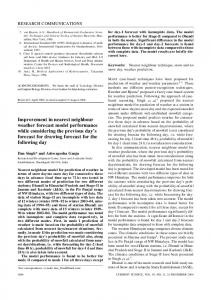
The two models can be explained using Figure 1. In Figures 1(a) to 1(d), we have assumed a total of five classes ('a' to 'e'). The samples of each class are represented by symbols 'a' to 'e'. The test pattern is shown as the square block around which a hypersphere is drawn to determine the number of neighbours included in the analysis. In a traditional nearest neighbour implementation, Figure 1(a) would assign the test pattern to class 'a' as there are two samples of class 'a' and only one sample of class 'b' within the boundary. Such decisions are based only on the number of nearest neighbours found. In Figure 1(b) we show the problem of neighbour conflict. In such cases, equal number of training neighbour are found for more than one class in class
determination of the test pattern. We term this a conflict. Conflicts can be resolved by either increasing the size of the hypersphere, i.e. involving more neighbours for a clear-cut decision, or by using conflict resolution described in kNN model above. Figure 1(c) shows aNN model process of finding the true class of the test pattern. Here the distance from a given class to the test pattern represents the averaged distance of all samples of that class found within the hypersphere. If all samples of a given class, e.g. 'e' in Figure 1(c), lie outside the hypersphere, then these are not included in the analysis. In all nearest neighbour methods, the number of neighbours analysed has a very important effect on the results of the analysis. This is shown in Figure 1(d). In this figure, when using the inner sphere, the class assignment for the unknown test pattern is 'a'. When we consider more neighbours with the outer sphere, the class assignment changes to 'd'. Thus, one important parameter to optimise in nearest neighbour methods is the number of neighbours included in the analysis. The above models will be analysed in this paper on image understanding data. The modified nearest neighbour methods will be used to classify unidentified data of natural objects (grass, trees, sky, river reflecting trees, and river reflecting sky) on the basis of training data available with samples coming from these five classes. The image understanding problem and the data used for this paper is explained in the next section.
A co-occurrence matrix [4] of a region of a single texture is widely recognised as having a characteristic texture which can be described using a variety of techniques [5]. In this research, the segmented regions are described using edge based co-occurrence matrices [6], an extension of the normal grey level co-occurrence matrix that allows greater flexibility in the description of the texture. The predominant form of these matrices is Gaussian with an overlaid higher level structure. The underlying Gaussian is due to Gaussian noise in the original imagery while the higher level structure is due to the texture of the originating region. It is this structure which most cooccurrence based texture measures seek to describe. The co-occurrence matrix structure is described using an orthogonal set of discrete Hermite functions defined on a lattice. The basis function of the Hermites is Gaussian and is used to describe the underlying Gaussian noise, while the higher order Hermites are used to describe the higher level structure of the matrix and hence the texture of the region [8].
f (n∆x, m∆y ) , centred at ( x0 , y 0 ) with standard deviations (σ x , σ y ) . This may be
Consider a function
decomposed functions:
into
pq
p
discrete
orthogonal
Hermite
q
f (n∆x, m∆y ) = ∑∑ f kl Φ k (n∆x − x0 )Φ l ( m∆y − y 0 ) l =0 k =0
…
3. Image Understanding The main thrust of our current work is on autonomous scene analysis. It is in this context that we evaluate the nearest neighbour methods. The aim is to develop intelligent systems that are capable of accurate recognition of various objects in natural scenes (see Becalick[1] for a survey of scene analysis research). The basic system consists of four parts: ! !
! !
Image acquisition and segmentation of major regions and boundaries in the image. The analysis and description of texture in the segmented region using discrete Hermite functions. The texture classification and object identification using nearest neighbour methods. The performance analysis of the classifiers on such data.
A sequence of FLIR imagery was segmented using edge based co-occurrence techniques [2,3] and resulted in the major regions and the boundaries being detected in a consistent manner. These segmented regions were then subjected to texture analysis in the feature generation and selection procedure described later.
(1)
where
f kl = ∑∑ f (n∆x, m∆y )Φ k (n∆x − x0 )Φ l (m∆y − y 0 ) m
n
…
(2)
provide a low-order feature vector descriptive of the texture in the region. The error η pq in the expansion is given by k
l
2 = ∑∑ ( f ( n∆x, m∆y ) − ∑∑ f kl Φ k ( n∆x − x0 )Φ l ( m∆y − y 0 )) 2 η pq m
k =0 l =0
l
…
(3)
Since
η pq =
∞
∞
∑∑ f
k = p 'l = q '
2 k ,l
, p ' > p, q ' > q …
(4)
then this error will remain the same, or decrease, if additional terms are used in the expansion, i.e.
η p ' q ' ≤ η pq , ∀( p' > p, q' > q ) …
(5)
These equations assume axes parallel to a square grid, co-occurrence matrices have axes along, and perpendicular to, the leading diagonal of the matrix. Accordingly, the above definitions are modified to include a translation along the x,y axis and a 45o rotation so that the axis of the basis function coincide with the natural axis of the co-occurrence matrix. Figure 2 shows the first few two-dimensional Hermite unctions (not to the same scale) and are used to decompose the co-occurrence matrices. Feature Selection and Generation The co-occurrence matrix decomposition techniques defined above provide a low order feature vector descriptive of the texture of a region. The zeroth order coefficient describes the Gaussian noise while the higher orders describe the texture and are used as the ‘raw’ features in the classification analysis described in this paper. The feature sets shown in table 1 were derived for training and test purposes.
4. Results Our previous analysis of the feature data shows that it is highly correlated and overlapping across different classes. In particular, it is difficult to separate vegetation (grass from trees) and reflection of trees in river from other vegetation. Linear methods are particularly worse with our data. In most trials with our image data, we found that average recognition rates vary between 40 to 50%. Past studies based on similar data have shown good results with neural networks [7]. In this study, we aim to demonstrate the following: (1) nearest neighbour methods perform robustly with increasing noise in test data; (2) comparative analysis of the two models proposed earlier. Table 2 shows the performance of kNN and aNN models and compares them with neural networks. The neural network model (three layer multilayer perceptron) has been optimised for its architecture and trained with backpropagation algorithm. A total of ten test sets are used with varying degrees of noise contamination. As mentioned earlier, the test sets are noise contaminated training data. For each feature, additive Gaussian noise is added to the training data as: ynew = y + y.δ.N where ynew is noise contaminated data, y is training data, δ is noise percentage (for 10% noise, δ=.1) and N is Gaussian noise vector.
The first column in Table 2 shows the percentage of noise in the test data. The next three columns are related to the performance of kNN model, the next column shows the performance of aNN model and the last two columns show performance of two baseline methods used in our study: standard nearest neighbour model (NN) and neural networks (Nnet). All nearest neighbour models have used a total of 3 nearest neighbours in their classification process. The second column shows the number of ties (conflicts) over the complete test run of 3777 patterns. It is interesting to note that as the amount of noise increases in test data, the number of ties increase almost linearly. In each of these situations, the kNN algorithm applies conflict resolution. Each time a tie is resolved in favour of one of the possible five classes, the system either makes the correct decision of choosing the true class or it makes a mistake of choosing the wrong class. The third column of Table 2, St shows in percentage the successful resolution of conflicts in favour of the true class of test data. This ability decreases with increasing noise. The fourth column R1 shows in percentage the recognition rate obtained by the kNN model. Considering the fact that for 1% noise, Linear Discriminant Analysis (LDA) gives a recognition rate of 41.4%, the results are encouraging. kNN recognition rates show a graceful degradation with increasing noise ranging between 81.3% to 76.4%. The next column in Table 2 shows recognition rates obtained using aNN model. The results for this model are the best ranging between 100% and 86.6% over the ten trials. The two new models kNN and aNN are now compared with two baseline models. The first baseline model is standard Nearest Neighbour model (NN) without conflict resolution assuming that in cases of conflict, the standard model has a 20% chance of correct classification with five classes. The results in this model are about 5 to 6% worse than kNN model. In the final column, the neural network baseline model (NNet) shows the results in a range between 89.1% and 54.7%. Their performance degrades very rapidly compared to the nearest neighbour models as noise increases. In general, overall performance of models degrade with increase in noise however successive trials with more noise may not necessarily lead to poorer performances (supported by other studies as for example [9]). For example, when noise increases from 4 to 5%, the nearest neighbour models improve their classification performances slightly. In general, the results shown in Table 2 are very convincing. They conclusively demonstrate the superiority of modified nearest neighbour models over their traditional counterparts or even neural networks on the given problem.
5. Conclusion In this paper we suggested two models of nearest neighbour classifiers and applied them to image understanding data. Our data was obtained by texture analysis of natural scenes and shows the properties of most real data in similar contexts, i.e. it is non-linear, strongly correlated across various features and overlapping across
various classes. The results shown in this paper for our two nearest neighbour models are extremely encouraging. One of the limitations is the limited amount of data available to us as well as the imbalance between patterns of various classes, e.g. there are many more patterns for vegetation compared to other classes. In future studies we propose to address this by developing synthetic data modelled on the basis of available real data. Such a database of synthetic data will allow further investigation with a range of classifiers including neural networks. Inspite of these limitations, we hope that this research contribution has highlighted the role of nearest neighbour methods for application in areas where noise management in data is an important factor. We are confident that further development along the lines suggested in this paper will lead to even more accurate and sophisticated classifiers.
References [1] DC Becalick, Natural Scene Classification using a Weightless Neural Network, PhD Thesis, Imperial College, Department o Electrical and Electronic Engineering, 1996. [2] JF Haddon, JF Boyce, Integrating Spatio-Temporal Information in Image Sequence Analysis for the Enforcement of Consistency of Interpretation, Special Issue of Digital Signal Processing, Oct 1998. [3] JF Haddon, JF Boyce, Image Segmentation by Unifying Region and Boundary Information, IEEE
Transactions on Pattern Analysis and Machine Intelligence, vol. 12, No 10, pp 929-948, 1990. [4] RM Haralick, K Shanmugan, I Dinstein, Texture Features for Image Classification, IEEE SMC-3, pp. 610621, 1973. [5] RM Haralick, Image Texture Survey, in Handbook of Statistics, vol. 2, P R Krishnaiah, L N Kanal, Eds., pp. 399-415, 1982. [6] JF Haddon, JF Boyce, Co-occurrence Matrices for Image Analysis, IEE Electronics and Communications Engineering Journal, vol. 5, No 2, pp. 71-83, 1993. [7] JF Haddon and JF Boyce, Texture Classification of Segmented Regions of FLIR Images using Neural Networks, Proceedings of the 1st International Conference on Image Processing, Texas, 1994. [8] JF Haddon, JF Boyce, Spatio-Temporal Relaxation Labelling Applied to Segmented Infrared Image Sequence, Proceedings of 13th International Conference on Pattern Recognition, IEEE Press, Austria. [9] S. Singh. Effect of Noise on Generalisation in Massively Parallel Fuzzy Systems, Pattern Recognition, vol. 31, issue 11, pp. 25-33, 1998. [10] S. Singh, A Single Nearest Neighbour Fuzzy Approach for Pattern Recognition, International Journal of Pattern Recognition and Artificial Intelligence, vol. 13, no. 1, pp. 49-54, 1999. [11] S. Theodoridis and K. Koutroumbas, Pattern Recognition, Academic Press, 1999.
Table 1. Feature Description in training and test data Originally 121 coefficients derived Training Data f kl , k, l = 0..10
Test Data
These coefficients are then analysed for their discriminatory power using linear discriminant analysis (LDA). A total of 42 features are then selected for final analysis. The data is normalised within the [0,1] range. A total of 3777 patterns are used. Each feature in the training data is contaminated by a Gaussian noise distribution (sd. = 1) to yield the test data. The noise added varies from 1 to 10% of the training data value. The test set size is the same as the training data, 3777 patterns (Grass = 1924, Tree = 1033, Sky = 273, River Reflecting Sky = 225, River Reflecting Trees = 321)
Table 2. Scene object classification performance of kNN, aNN and NN and NNet models NN% NNet % Noise % Ties Resolution % Recognition % Recognition % R1 R2 R3 R4 T St 1 242 100.0 81.3 100.0 76.2 89.1 2 233 100.0 81.3 99.9 76.4 85.3 3 237 100.0 81.0 99.4 76.0 79.1 4 243 99.5 80.7 98.6 75.5 73.9 5 253 100.0 81.0 97.5 75.6 69.0 6 266 98.4 80.5 96.2 74.8 64.8 7 282 96.0 79.9 93.7 73.9 61.3 8 282 92.9 78.9 91.2 72.9 59.2 9 304 88.4 77.4 89.2 71.0 57.1 10 294 84.0 76.4 86.6 70.2 54.7
Figure 1. k-nearest neighbour models and strategies: (a) Traditional k-nearest neighbour model; (b) Conflict resolution; (c) Closest average distance model; and (d) Hypersphere size effect on pattern recognition d d d d
(a)
d d
d d d d
(b)
d d d
d d
aa
aa a
b b b b c c c c
b b
a
a
b
a
b
b b e
c c
c e
e
(c)
c c c c
b e
c c
c e
e
(d) d d
d a
b
c
e
d dd
a
a
b
b
b
H00
d d d
e c c
c
H01 H10 Figure 2. The first few 2D Hermite functions
e
H11