Network Coding and Distributed Compression over ... - CalTech Thesis

Network Coding and Distributed Compression over Large Networks: Some Basic Principles

Thesis by

Mayank Bakshi

In Partial Fulfillment of the Requirements for the Degree of Doctor of Philosophy

California Institute of Technology Pasadena, California

2012 (Defended August 16, 2011)

c 2012

Mayank Bakshi All Rights Reserved

Dedicated to my family

Acknowledgements The work contained in this thesis was partially supported by NSF Grant Nos CCF-0220039, CCR0325324, and CNS-0905615, Darpa Grant No W911NF-07-I0029, and Caltech’s Lee Center for Advanced Networking. In addition, I would like to express my gratitude towards each and every person with whom I had the fortune of interacting during the course of my doctoral studies. In there own way, everyone I met and came to know made my stay at Caltech memorable and helped shape my research. At the risk of omitting many names, I would like to especially acknowledge the contribution of some key individuals. Without doubt, the greatest contribution in this regard was that of my advisor, Prof Michelle Effros. I have many fond memories of my interactions with her. Her principled approach towards everything, technical as well as non-technical, was often my guiding light. Her constant encouragement along with countless insightful discussions allowed me to develop deeper understanding of my research topics even when new ideas were not forthcoming. I also appreciate Prof Effros’ patient handling of the inevitable differences between her and mine approaches to certain problems. This understanding afforded me just enough flexibility to truly enjoy research, while ensuring that things kept progressing. Simultaneously, I had the privilege of working closely with Prof Tracey Ho. I would like to thank her for providing very valuable feedback throughout my doctoral research. On a similar note, I would also like to mention committee members Prof Shuki Bruck, Prof Mani Chandy, Prof Adam Wierman, Prof Babak Hassibi, and Prof Andreas Krause. I also had the pleasure of being part of many fruitful discussions with former group mates Sid, Wei-Hsin, and Asaf. These discussions kept the creative juices flowing and ultimately led to several new research ideas. Through Prof Effros, I came to know many other prominent researchers in my field. Of special mention are Prof Ralf Koetter, Prof Muriel Medard and Prof Alon Orlitsky. Interactions with them were crucial in shaping parts of the thesis. As a part my life as a Caltech student, I met many remarkable people. I learnt a lot through my former group mates Chris, Sukwon, Derek, Shirin, Ted, Tao, Svitlana, and Ming. Our meetings always led to interesting conclusions, both in research and outside of it. The EE staff, especially Shirley, Linda, and Tanya were instrumental in ensuring that logistics were take care of. Greg and

Christina at Caltech Y helped ensure that time was spent well even outside of research. The health center staff, especially Divina, also earn a special mention for keeping me fighting fit for the rigors of graduate life. I was extremely lucky to make several truly wonderful friends who helped me stay sane during this time. Sushree made sure I did not miss my family as I toiled towards my thesis completion. Uday and Prabha were there with me every step of the way since landing in Pasadena. Shankar and Shwetank were always ready with helpful advice whenever I needed. In no particular order, I would also like to acknowledge JK, Teja, Saha, Sowmya, Vijay, Arundhati, Samir, Mansi, Setu, Pinkesh, Zeeshan, Shwetank, Vikram, Krish, Sukhada, Arthur, Jean-Loup, and Ashish for memories that I will cherish for long. Last, but not the least, I would like to acknowledge my parent and my younger brother for constant support and nagging without which none of this would have been possible.

Abstract The fields of Network Coding and Distributed Compression have focused primarily on finding the capacity for families of problems defined by either a broad class of networks topologies (e.g., directed, acyclic networks) under a narrow class of demands (e.g., multicast), or a specific network topology (e.g. three-node networks) under different types of demands (e.g. Slepian-Wolf, Ahlswede-Körner). Given the difficulty of the general problem, it is not surprising that the collection of networks that have been fully solved to date is still very small. This work investigates several new approaches to bounding the achievable rate region for general network source coding problems - reducing a network to an equivalent network or collection of networks, investigating the effect of feedback on achievable rates, and characterizing the role of side information. We describe two approaches aimed at simplifying the capacity calculations in a large network. First, we prove the optimality of separation between network coding and channel coding for networks of point-to-point channels with a Byzantine adversary. Next, we give a strategy for calculation the capacity of an error-free network by decomposing that network into smaller networks. We show that this strategy is optimal for a large class of networks and give a bound for other cases. To date, the role of feedback in network source coding has received very little attention. We present several examples of networks that demonstrate that feedback can increases the set of achievable rates in both lossy and lossless network source coding settings. We derive general upper and lower bounds on the rate regions for networks with limited feedback that demonstrate a fundamental tradeoff between the forward rate and the feedback rate. For zero error source coding with limited feedback and decoder side information, we derive the exact tradeoff between the forward rate and the feedback rate for several classes of sources. A surprising result is that even zero rate feedback can reduce the optimal forward rate by an arbitrary factor. Side information can be used to reduce the rates required for reliable information. We precisely characterize the exact achievable region for multicast networks with side information at the sinks and find upper and lower bounds on the achievable rate region for other demand types.

Contents Acknowledgements

iv

Abstract

vi

1 Introduction

1

1.1

The Setup . . . . . . . . . . . . . . . . . . . . . . . . . . . . . . . . . . . . . . . . . .

1

1.2

Our contribution . . . . . . . . . . . . . . . . . . . . . . . . . . . . . . . . . . . . . .

4

1.2.1

Network Reduction . . . . . . . . . . . . . . . . . . . . . . . . . . . . . . . . .

5

1.2.2

Feedback in Network Source Coding . . . . . . . . . . . . . . . . . . . . . . .

5

1.2.3

Side Information in Networks . . . . . . . . . . . . . . . . . . . . . . . . . . .

6

2 Network Equivalence

7

2.1

Introduction . . . . . . . . . . . . . . . . . . . . . . . . . . . . . . . . . . . . . . . . .

7

2.2

Preliminaries . . . . . . . . . . . . . . . . . . . . . . . . . . . . . . . . . . . . . . . .

8

2.2.1

Network model . . . . . . . . . . . . . . . . . . . . . . . . . . . . . . . . . . .

8

2.2.2

Network code . . . . . . . . . . . . . . . . . . . . . . . . . . . . . . . . . . . .

9

2.2.3

Adversarial model . . . . . . . . . . . . . . . . . . . . . . . . . . . . . . . . .

10

2.3

Stacked network . . . . . . . . . . . . . . . . . . . . . . . . . . . . . . . . . . . . . .

11

2.4

Network equivalence . . . . . . . . . . . . . . . . . . . . . . . . . . . . . . . . . . . .

18

2.5

Equivalence for network source coding . . . . . . . . . . . . . . . . . . . . . . . . . .

21

2.5.1

Multicast Demands with Side Information at Sinks . . . . . . . . . . . . . . .

23

2.5.2

Networks with independent sources . . . . . . . . . . . . . . . . . . . . . . . .

24

2.5.3

An example where equivalence does not apply . . . . . . . . . . . . . . . . . .

24

3 The Decomposition Approach

28

3.1

Introduction . . . . . . . . . . . . . . . . . . . . . . . . . . . . . . . . . . . . . . . . .

28

3.2

Preliminaries . . . . . . . . . . . . . . . . . . . . . . . . . . . . . . . . . . . . . . . .

30

3.3

Results . . . . . . . . . . . . . . . . . . . . . . . . . . . . . . . . . . . . . . . . . . . .

31

3.3.1

31

Cutset bounds and line networks . . . . . . . . . . . . . . . . . . . . . . . . .

3.3.2

Independent sources, arbitrary demands . . . . . . . . . . . . . . . . . . . . .

33

3.3.3

Dependent sources, multicast . . . . . . . . . . . . . . . . . . . . . . . . . . .

34

3.3.4

A special class of dependent sources with dependent demands . . . . . . . . .

36

3.3.5

3-node line networks with dependent sources . . . . . . . . . . . . . . . . . .

38

3.3.6

Networks where additivity does not hold . . . . . . . . . . . . . . . . . . . . .

40

4 Feedback In Network Source Coding

42

4.1

Introduction . . . . . . . . . . . . . . . . . . . . . . . . . . . . . . . . . . . . . . . . .

42

4.2

Preliminaries . . . . . . . . . . . . . . . . . . . . . . . . . . . . . . . . . . . . . . . .

44

4.3

The role of feedback in source coding networks . . . . . . . . . . . . . . . . . . . . .

48

4.3.1

Source coding with coded side information . . . . . . . . . . . . . . . . . . . .

49

4.3.1.1

Networks with multicast demands . . . . . . . . . . . . . . . . . . .

54

4.4

Achievable rates for multi-terminal lossy source coding with feedback . . . . . . . . .

58

4.5

Finite feedback . . . . . . . . . . . . . . . . . . . . . . . . . . . . . . . . . . . . . . .

62

4.5.1

Upper and lower bounds . . . . . . . . . . . . . . . . . . . . . . . . . . . . . .

62

4.5.1.1

Upper bound . . . . . . . . . . . . . . . . . . . . . . . . . . . . . . .

62

4.5.1.2

Lower bound . . . . . . . . . . . . . . . . . . . . . . . . . . . . . . .

65

4.5.2

Zero-error source coding . . . . . . . . . . . . . . . . . . . . . . . . . . . . . .

65

4.5.3

Discussion . . . . . . . . . . . . . . . . . . . . . . . . . . . . . . . . . . . . . .

72

5 Side Information in Networks

74

5.1

Introduction . . . . . . . . . . . . . . . . . . . . . . . . . . . . . . . . . . . . . . . . .

74

5.2

Preliminaries . . . . . . . . . . . . . . . . . . . . . . . . . . . . . . . . . . . . . . . .

75

5.2.1

Network model . . . . . . . . . . . . . . . . . . . . . . . . . . . . . . . . . . .

75

5.2.2

Sources and sinks . . . . . . . . . . . . . . . . . . . . . . . . . . . . . . . . . .

75

5.2.3

Demand models

. . . . . . . . . . . . . . . . . . . . . . . . . . . . . . . . . .

75

5.2.3.1

Multicast with side information at the sinks . . . . . . . . . . . . .

77

5.2.3.2

Multicast with side information at a non-sink node

. . . . . . . . .

77

5.2.3.3

General demands

. . . . . . . . . . . . . . . . . . . . . . . . . . . .

77

Network source codes . . . . . . . . . . . . . . . . . . . . . . . . . . . . . . .

77

Multicast with side information at the sinks . . . . . . . . . . . . . . . . . . . . . . .

78

5.3.1

Achievability via random binning . . . . . . . . . . . . . . . . . . . . . . . . .

82

5.4

Multicast with side information at a non-sink node . . . . . . . . . . . . . . . . . . .

86

5.5

An inner bound on the rate region with general demand structures . . . . . . . . . .

90

5.6

Discussion . . . . . . . . . . . . . . . . . . . . . . . . . . . . . . . . . . . . . . . . . .

92

5.2.4 5.3

Bibliography

93

Chapter 1: INTRODUCTION

1

Chapter 1

Introduction 1.1

The Setup

Consider a communication system shown in Figure 1.1. Nodes 1 through m have source messages W (1) through W (m) available to them and wish to reconstruct functions f1 (W (1) , . . . , W (m) ) of all the source messages. Each edge in the network corresponds to a point-to-point channel whose inputs and outputs are related statistically according to transition probability pY |X . In order to achieve the communication objective, each node is allowed to perform the following coding operation. At (v)

(v)

time t, each ndoe v collects symbols Y1 , . . . , Yt−1 received at that node prior to time t, computes a (v)

function Xt

(v)

of these symbols, and transmits Xt

on outgoing edges from v. We call a transmission

scheme of this form a network code when the source messages are independent, and a network source code when the sources are dependent. Two figures of merits of network codes (and network source codes) that we consider are its error probability and rate. These terms are precisely defined later. Loosely speaking, the error probability of a network code (or a network source code) is the probability that at least one of the sinks incorrectly reconstructs its desired demands. The rate of a code measures its transmission efficiency. For a network code, this is typically measured in terms of the number of bits of each source message transmitted per time instant, while for a network source code it is usually measured as the number of transmitted codewords symbols transmitted per source symbol. In both these scenarios, the key quantity of interest to us is the set of achievable rates R, which is defined as the collection of rates for which there exist network codes with arbitrarily small error probability. The network model of Figure 1.1 may be thought of as a natural generalization of the point to point model of Figure 1.2. Shannon [1] showed that it is possible to reliably communicate a message in the presence of noise as long as the “amount of information" contained in the message is less than the “capacity" of the noisy channel. This model lends itself naturally to a vast number of channel coding and source coding scenarios – the two main themes explored in [1]. However, the above pointto-point model does not fully capture many network-based communication scenarios; the internet,


2

(1)

(1)

(m)

{f1 (Wk , . . . , Wk

(m)

{f3 (Wk , . . . , Wk

)}1 k=1

(3)

{Wk }1 k=1

(3)

{Xi }1 i=1

(1)

{Wk }1 k=1

1 {Xi(1) }1 i=1 PY (

3 4)

(1) 1 }i=1

{Yi

|X ( 1 )

(·|·)

(2)

{Xi }1 i=1

(3) 1 }i=1

{Yi

(1)

(m)

(m) 1 }i=1

{Xi

(m) 1 }i=1

{Yi

(2) {Yi }1 i=1

{f2 (Wk , . . . , Wk

...

4

2

(2)

{Wk }1 k=1

)}1 k=1

m (m) 1 }k=1

{Wk

)}1 k=1 (1)

(m)

{fm (Wk , . . . , Wk

)}1 k=1

Figure 1.1: A general multi-terminal communication model

W 1 , W2 , . . .

X 1 , X2 , . . . Transmitter

pY |X

Y 1 , Y2 , . . . Receiver

Figure 1.2: The point-to-point communication model

ˆ 1, W ˆ 2, . . . W


3

W (1)

1 3

W (1) , W (2) 2

W (2)

Figure 1.3: The Slepian-Wolf network

sensor networks, content distribution networks, and cellular networks are some examples of such systems. The following simple example makes this evident. Example 1 (Slepian-Wolf [6]). Consider the network shown in Figure 1.3. Node 1 and 2 observe (1)

(1)

∞ source processes {Wi }∞ i=1 and {Wi }i=1 , respectively. For each i = 1, 2, . . . ,, the pair of random (1)

(2)

variables (Wi , Wi ) is drawn independently from a known distribution pW (1) ,W (2) (·). Node 3 wishes to reconstruct both the sources. By the Source Coding Theorem [1], the smallest rates achievable on the edges (1, 3) and (2, 3) using the point-to-point approach are H(W (1) ) and H(W (2) ), respectively. On the other hand, Slepian and Wolf [6] show that all rates satisfying the following bounds allow recovering both W (1) and W (2) at the decoder: R1

≥ H(W (1) |W (2) )

R2

≥ H(W (2) |W (1) )

R1 + R2

≥ H(W (1) , W (2) ).

In particular, it follows that rates H(W (1) ) and H(W (2) |W (1) ) on edges (1, 3) and (2, 3), respec-

tively, are achievable. Since H(W (2) |W (1) ) < H(W (2) ) for a large class of interesting probability distributions, this illustrates that the point-to-point approach is suboptimal in general networked scenarios.

The sub-optimality of the point-to-point approach is also well established for general multiuser channels (see [7, 8]) and transmission over networks with more than one source-destination pair (see [9]). These further highlighting the inadequacy of point-to-point approach when dealing with multi-terminal data compression scenarios. While these examples make a compelling case for accomplishing general multi-terminal communication goals through schemes that are optimized taking the entire network into account, in practice, such an approach is hindered by rapid increase in complexity of analysis with increase in network size. Indeed, even the set of rates achievable using


4

W (1) 1

W

(2)

2

4

W (1)

3

W (3) Figure 1.4: A network with two side information sources

communication schemes that are optimized for the entire network is known for only a few special classes of networks. The following seemingly simple network is an example of a network for which the entire set of achievable rates is unknown till date. Example 2. Consider the network shown in Figure 1.4. Let W (1) , W (2) , and W (3) be sources observed at nodes 1, 2, and 3, respectively. Let PW (1) ,W (2) ,W (3) (·) be the joint distribution of these sources. Node 4 demands only W (1) . Let edges (1, 4), (2, 4), and (3, 4) be noiseless links. The set of achievable rates for this network is defined as the collection of rate triplets (R1 , R2 , R3 ) such that for every > 0, there exists a transmission scheme at rates R1 , R2 , and R3 bits per unit time on links (1, 4), (2, 4), and (3, 4), respectively, for which W (1) is reconstructed at node 4 with error probability at most . Traditionally, much of the research in analyzing general multi-terminal systems has focussed on solving networks such as the above by analyzing each such network separately. While considering networks one at a time has the advantage that resulting performance bounds and techniques are often specialized to the specific networks, it is perhaps also true that following this approach limits the class of networks that are well understood from an information-theoretic point of view. This motivates us to study properties that apply to general multi-terminal systems.

1.2

Our contribution

In this thesis, we attempt to gain insights into general networks by identifying several key informationtheoretic principles. Specifically, we explore the following ideas that are applicable to multi-terminal systems in varying generality.


1.2.1

5

Network Reduction

In Chapters 2 and 3, we consider two approaches towards solving general network problems by reducing them to potentially simpler problems. The approach considered in Chapter 2 shows that finding the adversarial network coding capacity of a network of independent point-to-point noisy channels is equivalent to finding the adversarial network coding capacity of another network which consists solely of error-free links of known capacity. This result extends previous works on this theme which deal with non-adversarial setups [10, 11]. This also shows that channels with same capacity are equivalent as far as their effect in network coding capacities are concerned. Combined with results of [10] and [11], this results enables us to focus our attention exclusively on networks of lossless links when the networks consists of point-topoint channels. In the rest of the thesis, we only consider networks of lossless capacitated links. In the spirit of the above equivalence, one is tempted to believe that an analogous result should also hold true for sources themselves, i.e., if two networks that have the same topology have the same source coding rate regions if the corresponding sources in the two networks have the same joint entropies. In Chapter 2, we formally state this notion and show that while this equivalence holds for some collection of sources, it fails for general data compression problems. Next, in Chapter 3, we explore the idea of decomposing a network into component networks and using the component networks to gain insights into for the original network. We focus specifically on Line Networks and show that for several classes of these networks, the set of achievable rates may be fully characterized using the decomposition approach. We also give counterexamples to show that this approach is suboptimal in general. Following the results from this chapter, the rest of the thesis focusses exclusively on networks of error-free links.

1.2.2

Feedback in Network Source Coding

In Chapter 4, we consider network source coding for error-free networks with feedback from sink nodes to source nodes. We present several examples of networks with unlimited feedback to demonstrate that the presence of feedback strictly increases the set of achievable rates in both lossy and lossless settings. We also observe that the presence of feedback can reduce the encoding and decoding complexity in some cases. Next, we derive general upper and lower bounds on the rate regions of networks with limited feedback demonstrating a fundamental tradeoff between the forward rates and the feedback rates. Finally we restrict our attention to zero-error source coding with limited feedback and decoder side information and derive the exact tradeoff between the forward rate and the feedback rate for several classes of sources. A surprising result is that even a zero-rate feedback can reduce the optimal forward rate by an arbitrary factor. Our results generalize prior works that focus largely on networks with two nodes [12, 13, 14, 15, 16, 17].


1.2.3

6

Side Information in Networks

Lastly, in Chapter 5, we focus on the role played by side information in network source coding problems. We first consider networks with multicast demands, i.e., all sinks want all sources, and characterize the exact rate region when each sink may have (possibly different) side information available to it. This result generalizes prior work on multicast networks without side information at the sinks [18] Next, we use this to derive a general achievable region for networks where side information may be present at a non-sink node in the network. Finally, we consider a general sourcedemand problem and use the results from the case with side information to derive an achievable rate region for this setup. We present our findings in the next four chapters. Each chapter explore a different fundamental aspect of multi-terminal communication systems. In the interest of keeping the notation for each chapter consistent with prior literature on that topic, the notation for each chapter is independently set up at the beginning of the chapter.

Chapter 2: NETWORK EQUIVALENCE

7

Chapter 2

Network Equivalence 2.1

Introduction

One common approach for communicating in networks of noisy channels is to separate network coding and channel coding. In this approach, we operate each channel essentially losslessly with the help of a channel code. We then perform network coding on an essentially noise-free network. Indeed, in [19, 10], this approach is shown to be asymptotically optimal when the noise values on the distinct channels of the network are independent of each other. It is also known that when channels corresponding to different links are not independent, operating the channel code for each link independently may be strictly suboptimal (see Example 2 in [10]). In these cases, the dependence between the noise values on different links is exploited by first creating an appropriate dependence between the transmitted codewords on these channels and then jointly decoding them at the receiver. In this chapter, we consider a network of independent point-to-point channels with the presence of a Byzantine adversary that observes all transmissions, messages, and channel noise values, and can corrupt some of the transmissions by replacing a constrained subset of the received channel outputs. The objective of the adversary is to maximize the probability of decoding error, and the capacity of the network is the set of vectors describing rates at which it is possible to reliably communicate across the network. It is tempting to believe that separation of network coding and channel coding is suboptimal in the case of our adversarial model due to the potential for statistical dependence between the "noise" observed on edges controlled by the adversary. We show, however, that the capacity of this network equals the adversarial capacity of another network in which each channel is replaced by a noise-free capacitated link of the same capacity. Thus, it is asymptotically optimal to operate the adversarial network code independently of the channel code in this framework. We do not assume any special structure on the topology of the network, e.g., we allow unequal link capacities and networks with cycles. We also allow arbitrary model of adversarial attack, e.g. edgebased or node-based attack. The result immediately extends previous adversarial network coding capacity results from noise-free networks (e.g. [20, 21, 22, 23, 24]) to that of networks of independent


8

point-to-point channels. The proof follows the strategy introduced in [19, 10]. In Section 2.3, we show that the adversarial capacity of a network is same as that of a stacked network comprised of many copies of the same network. In Section 2.4, we show that replacing one of the channels with a noiseless link of equal capacity does not alter the adversarial network coding capacity of the stacked network. We give a formal problem definition in Section 2.2. The above result also shows that the notion of Network Equivalence introduced by [19] extends beyond networks of independent channels, and exact equivalence holds even when an adversary may introduce arbitrary errors. A key assumption in both our result and the results of [19] is that all sources are independent. Jalali et al. [11] have extended the result to networks with dependent sources. Unlike the previous setups which are limited to independent sources, in networks with dependent sources, the joint distribution of sources (and not just their respective entropies) is needed in the design the network code. As a result, the achievability of a given collection of demands over a given network may depend critically on the joint distribution of the sources present. We illustrate this in Section 2.5 by with the help of an example.

2.2 2.2.1

Preliminaries Network model

We define a network N to be a pair (G, C). Here G = (V, E) is a directed graph with vertices {1, . . . , m} and directed edges E ⊆ V × V. Each edge e ∈ E describes the input and output of a point-to-point channel Ce . The full collection of channels is given by C = (Ce : e ∈ E).

For each e ∈ E, channel Ce is given by a vector (X (e) , Y (e) , Z (e) , Pe , Υe ), where X (e) , Y (e) , and

Z (e) are, respectively, the input, output, and noise alphabets of the channel, Pe is the probability distribution of the noise, and Υe : X (e) × Z (e) → Y (e) is the channel map that determines the

channel output as a function of the channel input and noise. The noise distribution Pe and mapping Υe together induce a conditional probability distribution of the channel output given the channel input, here denoted by pe (·|·). Thus, the random variables X (e) , Y (e) , and Z (e) denoting the input, the output, and the noise value of the channel, are related as Y (e) = Υe (X (e) , Z (e) ), with pe (y|x) =

Z

Pe (z)dz.

{z:Υe (x,z)=y}

(e)

For each t ∈ N+ and e ∈ E, let Xt

(e)

∈ X (e) , Yt

(e)

∈ Y (e) , and Zt

∈ Z (e) , respectively, be


9

the random variables denoting the transmitted, received, and noise values for edge e at time t. We assume that each transmission on edge e involves a delay of unit time and that the noise on all channels is independent and memoryless. Thus, (e)

(e)

(e)

Yt+1 = Υe (Xt , Zt ) ∀e ∈ E, t ∈ N+ and PE (Zτ(e) : e ∈ E, τ = 1, . . . , t) =

t YY

Pe (Zτ(e) ).

e∈E τ =1

Here, PE denotes the joint distribution of the noise values. For notational convenience, we adopt the following convention to represent collections of random vectors. For every collection of random variables Q1 , Q2 , . . . taking values from a set Q, we denote the row vector [Qt , Qt+1 , . . . , Qt+n−1 ] ∈ Qn by Qt:t+n−1 . We specify column vectors by underlining

them and the element of a given row from the column vector by parenthesis. Thus, Q ∈ QN

represents the column vector [Q(1), Q(2), . . . , Q(N )]T with Q(i) ∈ Q for all i. (v,∗)

For each v ∈ V and t ∈ N+ , let Xt

(v,w)

, (Xt

(∗,v)

: (v, w) ∈ E) and Xt

(u,v)

, (Xt

: (u, v) ∈ E)

denote the time-t random variables on edges outgoing from v and incoming to v, respectively; the Q (v,∗) (∗,v) (e) alphabets for Xt and Xt are X (v,∗) = u:(v,u)∈E X (v,u) and let Xt , (Xt : e ∈ E) denote (v,∗)

all transmitted random variables in the network at time t. Similarly, define Yt

(∗,v)

, Yt

(v,∗)

, Zt

,

(∗,v) Zt ,

Yt , and Zt for each v ∈ V and t ∈ N+ . Let X , X (u,∗) , and X (∗,v) denote the product sets Q Q (e) , v:(u,v)∈E X (u,v) , and v:(u,v)∈E X (u,v) . Similarly define Y, Y (u,∗) , Y (∗,v) , Z, Z (u,∗) , e∈E X

Q

and Z (∗,v) .

2.2.2

Network code

Let M = {(u, V ) : u ∈ V, V ⊆ V \ {u}} denote the set of possible pairs of source nodes and sink sets. A network coding solution S(N) implemented over n time steps is defined by message alphabet Q (u,v) W = (u,V )∈M W (u→V ) , the collection of encoder maps {ft : (u, v) ∈ E, t ∈ {1, . . . , n}} with (u,v)

ft

Y

:

V ⊆V

W (u→V ) ×

Y

v 0 :(v 0 ,u)∈E (u,v)

that determine the transmitted random variable Xt (∗,u)

V ⊆ V) and received vectors Y1:t g (u) :

Y

V ⊆V\{u}

0

(Y (v ,u) )t → X (u,v) as a function of the messages (W (u→V ) :

at node u, and the decoder maps {g (u) : u ∈ V } with

W (u→V ) ×

Y

v:(v,u)∈E

(Y (v,u) )n →

Y

V ⊆V:u∈V v∈V\{u}

W (v→V )


10

ˆ (v→V,u) : (v, V ) ∈ M, v ∈ V, u ∈ V ) as a function of that determine the reconstructed messages (W the messages (W (u→V

0

)

(∗,u)

: V 0 ⊆ V \ {u}) and received vectors Y1:t

u ∈ V. Let R = (R(u, V ) : (u, V ) ∈ M) ∈ R

|M|

at node u for all t = 1, . . . , n and

. We say that a solution S(N) is a rate R solution

if |W (u→V ) | = 2nR(u,V ) for all (u, V ) ∈ M. Without loss of generality, we assume that all messages are either binary vectors or binary matrices of appropriate dimensions.

2.2.3

Adversarial model

We assume an omniscient Byzantine adversary that observes all messages (W (u→V ) : (u, V ) ∈ M), noise values Z1:n , and the network code S in operation. Thus, the adversary can deduce all transmitted and received vectors, X1:n and Y1:n . The adversary picks a subset σ from the set Σ (e)

of permissible attack-sets and replaces the vectors (Yt

(e)

(e)

= Υ(Xt−1 , Zt−1 ) : e ∈ σ, t = 1, . . . , n) of (e)

channel outputs on these edges with the vector A1:n = (A1:n : e ∈ σ) of his own choice. The set Σ is known to the designer of the network code, but the chosen attack set σ ∈ Σ is unknown.

ˆ (v→V,u) 6= W (v→V ) for some v ∈ V, V ⊆ V \ {v}, and We say that there is a decoding error if W

u ∈ V . For a given solution S(N) that is implemented over n time steps, and for each (u, V ) ∈ M and

ˆ (u→V,v) is a deterministic function of the messages W = (W (u→V ) : (u, V ) ∈ M), the noise v ∈V, W (u→V,v)

values Z1:n , the attack-set σ, and the injected vector A1:n ; let GS

: W × Zn × Σ × Yn → W

denote this function. Since the adversary knows W and Z1:n , he can compute the decoded message for every possible choice of σ and A1:n . The adversary may then chose σ and A1:n to minimize the rate of reliable communication. We define the set E(S) ⊆ W × Z n as the collection of messages and noise values for which it is possible for the adversary to cause a decoding error for any of the messages, i.e., E(S) , (w, z1:n ) ∈ W × Z n : (u→V,v)

(w, z1:n , a1:n , σ) 6= w(u,V ) for some Y (u, V ) ∈ M, v ∈ V, σ ∈ Σ, and a1:n ∈ (Y (e) )n .

GS

e∈σ

The probability of error for the solution S(N) is PE (S) , =

Pr ((W, Z1:n ) ∈ E(S)) Z 1 X PE (z1:n )dz1:n . |W| {z1:n :(w,z1:n )∈E(S)}

W,Z1:n

w∈W

We say that a solution S(N) that is implemented over n time steps is a (λ, R)-solution if

|W

(u→V )

| = 2nR(u,V ) for every (u, V ) ∈ M and PE (S) < λ. The capacity region R(N) of a network

N is the closure of the set of all rate vectors R for which a (λ, R)-solution exists for every λ > 0.


11

v (y

P (u

,v )

| x)

u

N

(a) The original network N.

P (u

x (y |

v

)

,v )

u

N

(b) The stacked network N.

Figure 2.1: The stacked network N for a given network N

2.3

Stacked network

Following the proof method employed in [10], we define the stacked network as follows (See Figure 2.3). Let N = (G, C) be a network with vertex set V = {1, . . . , m} and edge set E. For each e ∈ E,

let P e be a probability distribution on (Z (e) )N obtained by forming an N -fold product of Pe with QN N itself, i.e., P e (z e ) = i=1 Pe (z e (i)) for all z e ∈ (Z (e)) . Next, let Υe : (X (e) )N × (Z (e) )N → (Y (e) )N represent a channel that maps pairs (xe , z e ) ∈ (X (e) )N × ∈ (Z (e) )N to Υe (xe , z e ) =

[Υe (xe (1), z e (1)), . . . , Υe (xe (1), z e (N ))]T . We define the N -fold stacked network N derived from N = (G, C) as a pair (G, C), where, G , G and C e , ((X (e) )N , (Y (e) )N , (Z (e) )N , P e , Υe ) for all e ∈ E.

For the network N, we denote the messages corresponding to the pair (u, V ) ∈ M by matrix

(u→V )

W 1:nR(u,V ) , and the transmitted, received, and noise values for the edge (u, v) ∈ E by matrices

X 1:n , Y 1:n , and Z 1:n respectively. Let N(1), N(2), . . . , N(N ) be N copies of the network N. For each (u→V )

i = 1, . . . , N , associate vector W 1:nR(u,V ) (i) with the message corresponding to the pair (u, V ) ∈ M, and X 1:n (i), Y 1:n (i), and Z 1:n (i), with the messages, and transmitted, received, and noise values, respectively, for the edge (u, v) ∈ E in N(i).

For ease of visualization, we think of N as a stack with layers N(1), N(2), . . . , N(N ) and infinite


P(

(y |

x)

12

v

) u,v

u

(y

P (u

,v )

N (1)

v

| x)

u

N (2)

.. . .. . P(

(y |

v

x)

) u,v

u .. .

P(

N (i)

.. .

(y |

x)

v

) u,v

u

N (N )

Figure 2.2: Visualizing N as a stack with N layers

capacity bidirectional edges connecting all N copies of a giveb vertex v ∈ V to each other as shown (v,∗)

in Figure 2.2. Thus, for each v ∈ V and i = 1, . . . , N , the transmitted vector X 1:n (i) may be a (v→U )

(∗,v)

function of all messages (W 1:nR(v,U ) : (v, U ) ∈ M) and received vectors Y 1:n .

The capacity region for the stacked network R(N) is normalized by the number of layers N .

In [10], it is shown that the capacity regions for N and N are equal when none of the edges are corruptible by the adversary. Even though the presence of an adversary changes the network capacity, the arguments of lemma 1 of [10] extend readily to our setup. We state this in the following Lemma without proof. Lemma 1. For any network N = (G, C), R(N) = R(N). Next, we show that there exists a sequence of solutions to the stacked network such that the error probability decays exponentially with the number of layers. In the non-adversarial case, the mutual


13

independence of (Z(i) : i = 1, . . . , N ) results in independent decoding errors for a solution that operates on each layer independently. Thus, applying a randomly generated error-correcting code (u→V )

to all messages (W 1:nR(u,V ) : (u, V ) ∈ M) before they are processed by the network code ensures an exponential decay of error probability [25]. However, in the presence of an adversary, decoding errors may no longer be independent across the layers. We overcome this difficulty by first designing a solution to the stacked network for which the error probability is maximum when decoding errors are statistically independent across layers, and then showing that, under this condition, the error probability for this solution decays exponentially in the number of layers. ˜ Theorem 1. Given any R ∈ int(R(N)), there exists a (2−N δ , R)-solution S(N) for N for some δ > 0 and for all N large enough. Proof. Let λ > 0 and let ρ > H(2λ), where H(·) is the binary entropy function. Let S(N) be a Q ˜ (λ, R)-solution for N with W = (u,V )∈M W (u→V ) = {0, 1}nR(u,V ) . We design the solution S(N) (u→V )

as follows. For each (u, V ) ∈ M, let w1:nR(u,V ) be a two-dimensional binary (1 − ρ)N × nR(u, V )

matrix. We first encode w(u→V ) by using a different error-correcting code for each column. Next, (u→V )

we transmit each row of the resulting binary matrices (w ˜ 1:nR(u,V ) : (u, V ) ∈ M) on a different layer using the solution S(N). Finally, we employ nearest-neighbor decoding at each node to reconstruct the messages. Code Construction: Fix a pair (u, V ) ∈ M and k ∈ {1, . . . , nR(u, V )}. Consider a binary

(u→V ) symmetric channel C˜ with crossover probability 2λ. Let Ψk : {0, 1}(1−ρ)N → {0, 1}N and (u→V )

Φk

: {0, 1}N → {0, 1}(1−ρ)N be the encoder and decoder mappings for an error-correcting code

for C˜ of blocklength N and rate (1 − ρ) that is designed randomly as follows. (u→V )

˜ Select W k

(u→V )

˜ ⊆ {0, 1}N of size 2(1−ρ)N by independently picking each element of W k

from

(u→V )

{0, 1}N using a uniform distribution. The encoder Ψk (u→V )

˜ a unique codeword ˜b ∈ W k

(u→V )

. The decoder Φk

maps each message b ∈ {0, 1}(1−ρ)N to ˆ maps each received vector ˜b ∈ {0, 1}N to the

reconstruction ˆb ∈ {0, 1}(1−ρ)N that corresponds to the nearest valid codeword. Let dH (·, ·) denote the Hamming distance between two binary vectors. In other words, (u→V )

Φk

ˆ (˜b) =

argmin ˆ b∈{0,1}nR(u,V )

(u→V )

dH Ψk

ˆ (ˆb), ˜b .

The encoding operation is shown in Figures 2.3. Q ˜ We construct the solution S(N) as follows. Let the message alphabet be W = (u,V )∈M W (u→V ) ,

where W (u→V ) , {0, 1}nR(u,V )×(1−ρ)N is the set of nR(u, V ) × (1 − ρ)N binary matrices. Let (u→V )

w1:nR(u,V ) ∈ {0, 1}nR(u,V )×(1−ρ)N be the message intended for the connection (u, V ) ∈ M. The ˜ solution S(N) performs the following sequence of operations:

(u→V )

(u→V )

1. For each pair of vertices (u, V ) ∈ M and message w1:nR(u,V ) ∈ W (u→V ) , let w ˜ 1:nR(u,V ) ∈


14

(u→V )

w1:nR(u→V ) (1) (u→V )

(u→V ) w1:nR(u,V )

w1:nR(u→V ) (2)

≡

...

...

...

...

.. .

.. .

.. . ...

(u→V )

w1:nR(u→V ) ((1 − ρ)N ) (u→V )

w1

.. . ... (u→V )

(u→V )

(u→V )

wnR(u,V )

wk

w2

. . . Ψ(u→V ) . . . k

(u→V )

w ˜1 (u→∗)

w ˜ 1:nR(u,V ) (1) (u→∗)

w ˜ 1:nR(u,V ) (2) (u→V ) w ˜ 1:nR(u,V )

≡

.. . (u→∗)

w ˜ 1:nR(u,V ) (N )

(u→V )

(u→V )

(u→V )

w ˜ nR(u,V )

w ˜k

w ˜2

...

...

...

...

.. .

.. . ...

Figure 2.3: The encoding operation for each message

.. . ...


{0, 1, }nR(u,V )×N with

15

(u→V )

w ˜k

(u→V )

= Ψk

(u→V )

wk

for each k = 1, 2, . . . , nR(u, V ). Thus, for each k, the code Ψk acts on the k-th column of the binary matrix w1:nR(u,V ) . This is illustrated in Figure 2.3. (u→V )

2. For each i = 1, . . . , N , communicate messages (w ˜ 1:nR(u,V ) (i) : (u, V ) ∈ M) using the solution (u→V )

ˆ S(N) on N(i). Let (w ˜ 1:nR(u,V ) (i) : (u, V ) ∈ M) be the reconstructed messages after operating S(N) on N(i). Figure 2.4(a) shows the layer-wise operation of S(N) on an edge (u, v) at time

step t < n and Figure 2.4(b) shows the layer-wise reconstruction at node u at the end of n time steps. 3. Finally, as shown in Figure 2.5, for every (u, V ) ∈ M, each vertex v ∈ V outputs a reconstruc(u→V,v)

tion w ˆ 1:nR(u,V ) ∈ {0, 1}nR(u,V )×(1−ρ)N with (u→V,v)

(u→V )

w ˆk

= Φk

ˆ˜ (u→V,v) , k = 1, . . . , nR(u, V ). w k

Analysis of error probability: Let (u, V ) ∈ M, v ∈ V and k ∈ {1, . . . , nR(u, V )}. Since C˜ is sym(u→V )

metrical and the input is uniformly distributed, the decoder Φk

maps each received vector to

the maximum likelihood estimate of the input given the received vector. By previous results on ˜

error exponents (See [25]), we know that such a code achieves an error probability of 2−N δ for some ˜ λ), since the rate 1 − ρ is less than the capacity 1 − H(2λ) of the channel C. ˜ Denote δ˜ = δ(ρ, (u→V ) (u→V ) ˆ ˜ the message and the received vector for the code (Ψ ,Φ ) by random variables B and B, k

k

ˆ˜ is statistically related to Ψ(u→V ) (B) respectively. B is uniformly distributed on {0, 1}(1−ρ)N ) and B k

˜ Let p ˜ denote the joint distribution of the message B and the reconstruction via the channel C. C (u→V ) ˆ ˜ Therefore, Φ (B. k

(u→V )

pC˜(B 6= Φk

ˆ˜ < 2−N δ . (B)) ˜

(2.1) (u→V )

We now show that the block error probability for the code (Ψk

(u→V )

) over the channel (u→V,v) (u→V ) ˜ ˆ 6= W k . Note that by the C is an upper bound for the block error probability Pr W k (u→V )

choice of the solution S(N), Pr(W k

(u→V )

max Pr W k

b∈{0,1}

, Φk

ˆ (u→V,v) (i)) < λ for each i = 1, . . . , N . Thus, (i) 6= W k

ˆ (u→V ) (i)|W (u→V ) (i) = b < 2λ (i) 6= W k k

for each i = 1, . . . , N . Let wH (·) denote the number of 1’s in a binary vector. For every ˜b ∈ (u→V )

Wk

(u→V )

, let πk

(˜b) ⊆ {0, 1}N denote the set of all minimal weight error patterns that are (u→V )

decoded incorrectly by Φk following:

(u→V )

, i.e., πk

(˜b) is the set of all vectors e ∈ {0, 1}N satisfying the


16

v (u→∗)

w ˜ 1:nR(u,V ) (1) (u,v)

(∗,u)

Y 1:t (1)

u

Xt

(1) N (1), S(N )

v

(u→∗)

w ˜ 1:nR(u,V ) (2) (u,v)

(∗,u)

Y 1:t (2)

u

Xt

(2) N (2), S(N )

.. . v

(u→∗)

w ˜ 1:nR(u,V ) (i) (u,v)

Y

(∗,u) 1:t (i)

u

(u,v)

(∗,u)

(u→∗)

(∗,u)

(w ˜ 1:nR(u,V ) (i), Y 1:t (i))

v

w ˜ 1:nR(u,V ) (N ) Y 1:t (N )

(i) = ft

N (i), S(N )

.. .

(u→∗)

(u,v)

Xt

u

Xt

(N ) N (N ), S(N )

(u,v)

(a) The time-t transmitted vector X t (i) on an edge (u, v) not attacked by the adversary in the i-th layer is a function only of the received vectors and input messages at the vertex u in the i-th layer until time-step t. (u→∗)

w ˜ 1:nR(u,V ) (1)

u

v

(∗,u)

Y 1:n (1) (u→∗) w ˜ 1:nR(u,V ) (2) (∗,u) 1:n (2)

Y

N (1), S(N )

ˆ (∗→∗,u) (1) w ˜ 1:nR(u,V ) u

v N (2), S(N )

(∗→∗,u) ˆ w ˜ 1:nR(u,V ) (2)

.. . (u→∗)

w ˜ 1:nR(u,V ) (i) Y

(∗,u) 1:n (i)

(u→∗) w ˜ 1:nR(u,V ) (N )

u

v

ˆ (∗→∗,u) (i) w ˜ 1:nR(u,V ) .. .

N (i), S(N )

v u

(∗,u)

Y 1:n (N ) (∗→∗,u) ˆ w ˜ 1:nR(u,V ) (N )

N (N ), S(N )

(b) The decoded messages for the i-th layer solution S(N) depend only on the received vectors and input messages seen at the vertex u in the i-layer over the entire blocklength n.

Figure 2.4: The layer-by-layer operation of the stacked solution


(u→V,v) ˆ w ˜ 1:nR(u,V )

17

(u→V,v) ˆ w ˜ 1:nR(u,V ) (1)

...

...

ˆ (u→V,v) (2) w ˜ 1:nR(u,V )

...

...

≡

.. .

.. .

.. .

(u→V,v) ˆ w ˜ 1:nR(u,V ) (N )

... ˆ˜ (u→V,v) w ˆ˜ (u→V,v) w 1 2

.. . ... (u→V,v) w ˜ˆ nR(u,v)

ˆ˜ (u→V,v) w k

. . . Φ(u→V ) . . . k

(u→V,v)

w ˆ1

w ˆ nR(u,V )

w ˆk

(u→V,v)

...

...

(u→V,v)

...

...

w ˆ 1:nR(u→V ) (1) w ˆ 1:nR(u→V ) (2) (u→V,v) w ˆ 1:nR(u,V )

(u→V,v)

(u→V,v)

(u→V,v)

w ˆ2

≡

.. . (u→V,v)

w ˆ 1:nR(u→V ) ((1 − ρ)N )

.. .

.. . ...

.. . ...

(u,V ) ˆ˜ (u→V,v) )1:nR(u,V ) after performing Functions Φk finally map the layer-by-layer reconstructions w (u→V,v) the stacked solution to decoded messages w ˆ )1:nR(u,V ) at each node v.

Figure 2.5: The decoder operation for each message


18

(u→V )

(u→V ) ˜ (˜b) 6= Φk (b ⊕ e)

(u→V )

(u→V ) ˜ (˜b) = Φk (b ⊕ ˜e) for all ˜e such that {i : e˜(i) = 0} ⊇ {i : e(i) = 0}.

1. Φk 2. Φk

(u,V )

Let c ∈ {0, 1}N . Then the probability that W k

is decoded incorrectly for some adversarial

˜ (u,V ) is c is bounded from above by the strategy on network N when the transmitted vector W k ˜ (u,V ) is transmitted over the channel C˜ as follows: probability of error when W k (u,V ))

Pr(W k

ˆ (u→V,v) |W ˜ (u,V ) = c) 6= W k k

(u→V )

= Pr(Φk X =

(u→V )

e∈πk

≤

X

(u→V )

e∈πk

(c)

(u→V )

) 6= Φk

ˆ˜ (W k

(u→V,v)

(u→V )

˜ )|W k

= c)

ˆ˜ u→V,v (i) = c(i) ⊕ e(i)} Pr ∩i:e(i)=1 {W k

˜ (u→V ) = c} W k

(2λ)wH (e)

(2.2)

(c)

(u→V )

= pC˜ Φk

(u→V )

˜ (W k

(u→V )

(c) 6= Φk

ˆ˜ (W k

(u→V,v)

(u,V )

˜ )|W k

=c .

(2.3)

Therefore, (u,V ))

Pr(W k

ˆ (u→V,v) |W ˜ (u,V ) = c) < 2−N δ˜. 6= W k k

The bound in (2.2) is a consequence of the fact that for each i = 1, . . . , N and k = 1, . . . , nR(u, V ), ˆ˜ (u→V ) (i)} depends only ˜ (u→V ) (i) 6= W whether or not the adversary’s actions can cause the event {W k

k

˜ (i), and can occur with probability at most 2λ under on the noise values Z1:n (i) and the messages W

all possible adversarial actions. Step (2.3) follows from the fact that the transition probability for the channel C˜ is 2λ. Finally, applying a union bound over all values of k and (u, V ), we obtain ˜

˜ ≤ n|M|2−N δ PE (S)

max R(u, V ) ≤ 2−N δ

(u,V )∈M

for every δ < δ˜ for large enough N .

2.4

Network equivalence

In this section, we prove that finding the capacity region of the network N is equivalent to finding the ˆ R where one of the links eˆ = (1, 2) is replaced by a noiseless links of capacity capacity of a network N R = C(ˆ e). Koetter et al. [10] prove this by first showing that for every R < C(ˆ e), the capacity region ˆ R is a subset of that of N. Next, they show that for every R > C(ˆ of the N e), the capacity region of ˆ R . We follow a similar proof outline for our case. The proof of the first N is a subset of that of N


19

part follows the arguments of [10] exactly. We state it without proof in the following theorem. ˆ R defined above, R(N ˆ R ) ⊆ R(N) if R < C. Theorem 2. For the networks N and N ˆ R ) ⊇ R(N) if R > C, Koetter et al.argue that a noisy channel may be Next, to prove that R(N

emulated on the lossless link eˆ in the stacked network NR by using a randomly generated source (u,v)

code that operates across the layers. Their proof relies on typicality of the vector X t

, which

follows from the statistical independence of random variables corresponding to different layers. This assumption is not true in our case because the adversary may introduce dependence between different layers. To accommodate this possibility, we modify the proof of [10] to use a universal source code that first determines the type of the received sequence and then emulates the channel using a source code designed specifically for the observed type. We assume here that the alphabet X (ê) is finite. ˆ R defined above, R(N ˆ R ) ⊇ R(N) if R > C. Theorem 3. For the networks N and N ˆ∈ Proof. First, we design a sequence of universal source codes {(αN,t , βN,t )}t=1,2,... , each at rate R (C(ˆ e), R), that operate by describing the type of the input followed by the index of the codeword picked from a codebook designed for that type. Next, we modify a given (2−N δ , R)-solution S(N)

ˆ for N to a solution S(N ˆ by the source codes R ) for NR by emulating the channel on the link e

ˆ {(αN,t , βN,t )}t=1,2,... . Finally, we conclude that the error probability for the solution S(N R ) vanishes as N grows without bound.

−N δ ˆ , R)-solution to N implemented over n time steps Construction of S(N R ): Let S(N) be a (2

and obtained from the solution S(N) by following the construction in Theorem 1. We modify S(N) ˆ to obtain a solution S(N R ) by first designing a sequence of universal source codes {αN,t , βN,t }t=1,2,...

ˆ ∈ (C(ˆ that operate at a rate R e), R) and next appending the above source code to S(N) to emulate ˆ . the channel conditional probability peˆ on the the channel Cêˆ in network N R

Design of {αN,t , βN,t }t=1,2,... : Let PN be the set of all types of N length sequences from X (ê) .

ˆ For a vector x ∈ (X (ê) )N , let Q(x) ∈ PN denote the empirical distribution of x. Let Q ∈ PN . Let

(XQ , YQ ) be random variables jointly distributed on X ( eˆ) × Y ( eˆ) such that Pr(XQ = x) = Q(x) and the conditional distribution of YQ given XQ is peˆ. For each t = 1, . . . , n, select BtQ ⊆ (Y ( eˆ))N by ˆ

(N )

choosing 2N R elements uniformly at random from A

(YQ ).

For t = 1, . . . , n, let the encoder αN,t : (X (ê) )N → {0, 1}|X

(ˆ e)

| log2 (N +1)

ˆ

× {1, . . . , 2N R }

consist of the pair of maps to (αP , αB ), where, for each x ∈ (X (ê) )N , αP (x) is the binary description

ˆ Q(x) (N ) ˆ of Q(x), such that (x, yˆ) ∈ A (XQ(x) , YQ(x) ). If and αB (x) is the index of some vector yˆ ∈ Bt ˆ ˆ


20

no such vector yˆ exists, then αB (x) is set to be 1. Next, let the decoder βN,t : {0, 1}|X

(ˆ e)

| log2 (N +1)

ˆ

× {1, . . . , 2N R } → (Y (ê) )N

map pairs (xP , xB ) to the vector with index xB in BtQ , where Q is the type described by xP .

ˆ ) is identical to S(N) except for the ˆN Appending {αN,t , βN,t }t=1,2,... to S(N): The solution S( R

maps at nodes 1 and 2. For (u, v) ∈ V × V, let f (u,v) : W (u→∗) × (Y (∗,u) )nN → (X (u,∗) )nN denote

the encoder that determines the codeword on the edge (u, v) and let g (u) : W (u→∗) × (Y (∗,u) )nN → Q (∗→{u}∪V ) denote the decoder for the messages meant for node u in the solution S(N). V ⊆V\{u} W

ˆ (e) = X (e) and Yˆ (e) = Y (e) for all e 6= eˆ. Let X ˆ (ê) = f (1,2) (W 1→∗ , Yˆ (∗,1) )) and Yˆ (ê) = Let X 1:n 1:n 1:n 1:n t 1:n 1:n

ˆ R ) be a solution with encoder and decoder mappings (fˆ(u,v) : (u, v) ∈ ˆ (ê) )). Let S( ˆN βN,t−1 (αN,t−1 (X t−1

E) and (ˆ g (u) : u ∈ V), where,

(∗,u) fˆ(u,v) (W (u→∗) , Yˆ 1:n ) ,

and

 (∗,u)   f (u,v) (W (u→∗) , Yˆ 1:n )       if (u, v) 6= eˆ and u 6= 2      α(f (u,v) (W (u→∗) , Yˆ (∗,u) )) 1:n   if (u, v) = eˆ    (∗,u)    f (u,v) (W (u→∗) , Yˆ 1:n )      if u = 2

 (∗,u)   g (u) (W (u→∗) , Y 1:n )      if u 6= 2 (∗,u) (u→∗) (u) gˆ (W , Y 1:n ) , (u)  g (W (u→∗) , Yˆ (∗,u) )   1:n     if u = 2. [ˆ e]

(e)

Analysis of error probability: Let t = 1, . . . , n. Let Z1:n = (Z 1:n : e ∈ E \ {ˆ e}) be the noise

values on all edges except the edge eˆ and let W = (W (u→V ) : (u, V ) ∈ M) denote the collection of

ˆ (ê) is a deterministic function of W , Z[ê] , and transmitted messages. Note that for t = 1, . . . , n, X 1:t 1:t−1

(ˆ e) (ˆ e) ˆ Let pˆt denote the conditional Yˆ 1:t−1 while Yˆ 1:t is a random variable due to the random design of S.

ˆ ˆ probability distribution of Yˆ t given X t−1 under a random choice of S as described above. By Lemma 11 in [10], pˆt (ˆ y t |ˆ xt−1 ) ≤

N Y

i=1

peˆ(ˆ y t (i)|ˆ xt−1 (i)) · 2N a(,N,t) . (N )

for every (ˆ xt , yˆt−1 ) such that x ˆ t ∈ (X ( eˆ))N and (ˆ xt−1 , yˆt ) ∈ A

(XQ(x ˆ

t−1 )

, YQ(x ˆ

t−1 )

). Further, since

R > C(ˆ e), by standard random coding arguments (e.g., proof of Rate Distortion Theorem, [26]), for


21

large enough N , ) pt {ˆ y t : (ˆ yt , x ˆ t−1 ) ∈ / A(N (XQ(x ˆ

t−1 )

, YQ(x ˆ

t−1 )

}|ˆ xt−1 ) ≤

(ˆ e)

Next, note that messages w, noise values z[ê] = (z (e) : e ∈ E \ eˆ), transmitted vector x1:n ,

e) and received vector y (ˆ result in a decoding error under the solution S if there exists z(ê) such 1:n

(ˆ e) (ˆ e) ˆ w, z[ê] ) = {z(ê) : (w, z[ê] , z(ê) ) ∈ that (w, z[ê] , z(ê) ) ∈ E(S(N)), and y t(ê) = Υeˆ(xt−1 , z t−1 ). Let E(S,

ˆ ) for given values ˆN E(S(N))}. The expected probability of a decoding error over the choice of S( R [ˆ e]

of z1:n and w is given by Z

[ˆ e] ) ˆ E(S,w,z

≤

Z

Y n

t=1

[ˆ e] ) ˆ E(S,w,z

(ˆ e) (ˆ e) (ˆ e) pˆt (Υeˆ(zt−1 )|ˆ xt−1 ) dz1:n

Y n Y N

t=1 i=1

(ˆ e) (ˆ e) (ˆ e) peˆ(Υeˆ(zt−1 (i), x ˆt−1 (i))|ˆ xt−1 (i))2N a(,N,t)

(ˆ e)

dz1:n + .

[ˆ e]

Taking expectation over W and Z1:n , X h −nN P ˆ (u,V )∈M R(u,V ) ES,W 2 ˆ ,Z1:n PE (S) = w

Z

z:(z,w)∈E(S)

Y n Y N

(ˆ e)

(ˆ e)

(ˆ e)

peˆ Υ(zt−1 (i), x ˆt−1 (i))|ˆ xt−1 (i)

t=1 i=1

i [ˆ e] 2N a(,N,t) PE (z1:n ) dz1:n +

= PE (S) · 2nN c(,N ) + .

Since we assumed that S is a (2−N δ , R) solution, we get −N δ ˆ ES,W · 2nN a(,N,t) + . ˆ ,Z1:n PE (S) ≤ 2 Finally, for a fixed value of n, let < 1/n, and choose N large enough to conclude that R ∈ ˆ ). R(N R

2.5

Equivalence for network source coding

In point-to-point source coding (Figure 1.2), all rates greater than the entropy of the source are sufficient to successfully describe the source losslessly. As a result, from the point of view of rate calculation, all sources with the same entropy are equivalent.


22

Note that the number of typical sequences of length n for a memoryless source W is roughly equal to 2nH(W ) . Further, by the Asymptotic Equipartition Property (henceforth, AEP) [27], the observed sequence lies in the set of typical sequence with probability approaching one asymptotically. Thus, from a coding point of view, the notion of equivalence is further reinforced by noting that a code designed for a source W (1) can be applied to another source W (2) of the same entropy by first mapping typical sequences for W (1) to typical sequences for W (2) and then employing the code designed for W (1) . This property is especially useful in systems with multi-step coding as it enables the system designer to design subsequent encoders independently of the exact source distribution. For example, in designing the channel code, it suffices to restrict the attention to sources that are uniformly distributed binary vectors of length equal to the binary entropy of the source. This motivates us to examine whether a similar property holds for network source coding problems as well. Here, we restrict our attention to networks of error-free links. For a network N defined over the graph G = (V, E) with sources (W (v) : v ∈ V) distributed according to a joint distribution

PV (·), we define the achievable rate region R(N) ⊆ R|E| as the set of rate vectors such that for each R = (Re : e ∈ E) ∈ R(N) and for every λ > 0, there exists a network source code that meets the desired demands with error probability at most λ. For a precise definition, the reader is referred to Chapters 4. To formalize notion of equivalence for this setup, let N1 and N2 be two networks defined on isomorphic graphs G1 = (V1 , E1 ) and G2 = (V2 , E2 ), respectively. Let I : V1 → V2 be the one-to-one map from V1 to V2 associated with the isomorphism of G1 and G2 . For each v ∈ V1 ∪ V2 , let W (v) be a random variable observed at node v such that the collections of random variables

(W (v) : v ∈ V1 ) and (W (v) : v ∈ V2 ) are distributed according to probability mass functions PV1 and PV2 , respectively. Definition 1 (Networks with Isomorphic Demands). We say that N1 and N2 are networks with isomorphic demands if the following are true: 1. N1 and N2 are defined on isomorphic graphs. 2. For each pair of vertices (u, v) ∈ V1 , the source W (u) is losslessly present as a lossless demand at vertex v in N1 if and only if W I(u) is present as a lossless demand at vertex I(v) in N2 .

For each i ∈ {1, 2}, H(Ni ) denote the entropic vector for sources in Ni , i.e., H(Ni ) = (H(W (v) : v ∈ V ) : V ⊆ V) for i = 1, 2. Thus, the entropic vector for a given network consists of the collection of all possible joint entropies corresponding to the sources associated with the network. Note that the entropic vector captures the AEP for multiple sources in much the same way as the entropy does for a single source. For example, the number of jointly typical sequences of length n corresponding to sources (W (v) : v ∈ V )


X (s1 )

X (s2 )

23

X (t1 )

s1

t1 t2

.. .

X (sk )

s2

.. .

N

sk

(X (s) : s ∈ S) (X (s) : s ∈ S)

X (t2 ) tm

(X (s) : s ∈ S)

X (tm ) Figure 2.6: A multicast network with side information at the sinks

is approximately equal to 2nH(W

(v)

:v∈V )

for every V ⊆ V. Similarly, the probability of observing

jointly typical sequences approaches one as the blocklength n grows without bound. Thus, it is tempting to believe that the following proposition holds: Proposition 1. Let N1 and N2 be networks with isomorphic demands, and let H(N1 ) = H(N2 ). Then, R(N1 ) = R(N2 ).

In the rest of the section, we examine the correctness of the above proposition under various conditions.

2.5.1

Multicast Demands with Side Information at Sinks

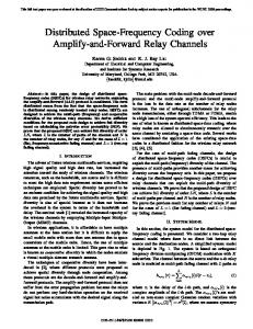
Let N1 and N2 be networks networks with isomorphic demands. Let T1 ⊆ V1 and T2 , {I(v) : v ∈ T1 } be the set of sink nodes in N1 and N2 , respectively.

Definition 2 (Multicast demands with side information at the sinks). We say that N1 and N2 have multicast demands with side information at sinks if all sources in the collection (W (v) : v ∈ / T1 )

(resp. (W (v) : v ∈ / T2 )) is demanded at all vertices in T1 (resp. T2 ). See Figure 2.6 for an example

of a multicast network. Note that the above definition allows side information at the sink nodes. The rate region for this setup is characterized in Chapter 5. As a corollary of this characterization, Proposition 1 follows. We state this as the following lemma. Lemma 2. Let N1 and N2 be multicast networks with isomorphic demands and let H(N1 ) = H(N2 ). Then, R(N1 ) = R(N2 ).


24

Proof. The proof follows directly from the fact that that rate regions for both N1 and N2 are fully characterized in terms of their respective source entropies.

2.5.2

Networks with independent sources

Let N1 and N2 be networks with isomorphic demands and independent sources satisfying the conditions of Proposition 1. By Corollary 2.3.3 of [28], it follows that the above proposition holds.

X (1)

1

3

X (2)

X (4)

N1

ˆ (4) X

N2

2

4

6

X (5)

ˆ (1) X

5

Figure 2.7: Two isomorphic networks with coded side information

2.5.3

An example where equivalence does not apply

Next, we show that 1 does not hold for all source distributions and for all demand scenarios. In particular, we consider two instances of the Ahlswede-Körner network of [29] and show that the rate regions for these are different even though the entropic vectors are the same. Example 3. Consider the coded-side information networks N1 and N2 shown in Figure 2.7. Let W (1) , W (2) , W (4) , and W (5) be random variables defined on alphabets W (1) , W (2) , W (4) ,

and W (5) respectively. Let each of these alphabets be equal to {w1 , w2 , w3 , w4 }. Let W (1) and W (4)

be distributed uniformly over their respective source alphabets. Let W (2) be jointly distributed with W (1) according to the conditional probability distribution

pW (2) |W (1) (wj |wi )

=

   1/2   1/2     0

if i, j ∈ {1, 2} if i, j ∈ {3, 4} otherwise.


25

Let W (5) be jointly distributed with W (4) according to the conditional probability distribution

pW (5) |W (4) (wj |wi )

   1/2   = 1/2     0

if j = i if j = i + 1(mod 4) otherwise.

Consider network N1 consisting of the sources W (1) and W (2) observed at vertices 1 and 2, respectively, and lossless demand W (1) at vertex 3. Similarly, network N2 consists of the sources W (4) and W (5) observed at vertices 4 and 5, respectively, and demand W (4) at vertex 6 By [29], R(N1 ) is the set of rate pairs (R(1,3) , R(2,3) ) such that R(1,3)

≥

H(W (1) |U )

(2.4)

R(2,3)

≥

I(W (2) ; U )

(2.5)

for some random variable U forming the Markov chain W (1) → W (2) → U . Similarly, R(N2 ) is the set of rate pairs (R(4,6) , R(5,6) ) such that R(4,6)

≥ H(W (4) |V )

(2.6)

R(5,6)

≥ I(W (5) ; V )

(2.7)

for some random variable V forming the Markov chain W (4) → W (5) → V .

Claim: There exist random variables (W (1) , W (2) ) and (W (4) , W (5) ) satisfying: H(W (1) ) = H(W (4) ), H(W (2) ) = H(W (5) ), and

H(W (1) , W (2) ) = H(W (4) , W (5) ),

such that R(N1 ) 6= R(N2 ). Proof. Let W (1) and W (4) be uniformly distributed on {1, 2, 3, 4}. Let W (2) and W (5) be random

variables taking values in {1, 2, 3, 4} and related to W (1) and W (4) through the transition proba-

bilities PW (2) |W (1) (·|·) and PW (5) |W (4) (·|·) shown in Figures 2.8 and 2.9 .

It is easy to verify that

H(W (1) ) = H(W (4) ) = H(W (2) ) = H(W (5) ) = 2 and H(W (1) , W (2) ) = H(W (4) , W (5) ) = 3. By (2.4) and (2.5), for every (R(4,6) , R(5,6) ) ∈ R(N2 ), R(4,6) + R(5,6) ≥ H(W (4) |V ) + I(W (5) |V )

(2.8)

for some V s.t. W (4) → W (5) → V is a Markov chain. The first term on the right-hand side of the


pX (1) (·) 1/4

X (1)

26

pX (2) |X (1) (·|·)

X (2)

pX (2) (·)

1/2

x1

1/2

x1

1/4

x2

1/4

x3

1/4

x4

1/4

1/2 1/4

x2

1/4

x3

1/2

1/2 1/2 1/2

1/4

1/2

x4

Figure 2.8: Transition probabilities for W (2) given W (1) for network N1

pX (4) (·)

pX (5) |X (4) (·|·)

X (4)

1/4

x1

1/4

x2

X (5)

pX (5) (·)

x1

1/4

x2

1/4

x3

1/4

x4

1/4

1/2 1/2

1/2 1/2

1/4

1/2

x3

1/2

1/2 1/2 1/4

x4

Figure 2.9: Transition probabilities for W (5) given W (4) for network N2


27

above equation can be lower bounded as follows: H(W (4) |V )

=

4 X 4 X i=1 j=1

=

PV (i)PW (4) |V (j|i) log

1 PW (4) |V (j|i)

1 1 PV (i) PW (5) |V (j|i) + PW (5) |V (j(mod 4) + 1|i) 2 2 i=1 j=1

4 X 4 X

4

≥ 1+

4

1 XX PV (i)PW (5) |V (j|i) 2 i=1 j=1 log

PW (5) |V (j|i) +

1 2 PW (5) |V

log

1 2 PW (5) |V

1 (j(mod 4) + 1|i)

1

(j|i) + 12 PW (5) |V (j(mod 4) + 1|i)

PW (5) |V (j(mod 4) + 3|i) .

Now, consider rate points (R(4,6) , R(5,6) ) for which R(4,6) ≤ 1. Note that when H(W (4) |V ) = 1, the above implies that PW (5) |V (j|i) = 0 or 1. Thus, I(W (5) ; V ) = 2. Therefore, if R(4,6) ≤ 1, R(4,36 + R(5,6) ≥ 3.

(2.9)

Next, note that (1, 1) ∈ R(N1 ). This can be seen by choosing a binary valued U that is a

deterministic function of W (2) as follows:

Thus,

  0 U=  1

if W (2) ∈ {1, 2}

if W (2) ∈ {3, 4}.

H(W (1) |U ) = H(U ) = 1, and I(W (2) ; U ) = H(U ) − H(U |W (2) ) = 1. Clearly, (1, 1) ∈ / R(N2 ), as it violates (2.9). Thus, R(N1 ) 6= R(N2 ).

Chapter 3: THE DECOMPOSITION APPROACH

28

Chapter 3

The Decomposition Approach 3.1

Introduction

It is fair to say that the field of network coding has focused primarily on finding solutions for families of problems defined by a broad class of networks (e.g., networks representable by directed, acyclic graphs) and a narrow class of demands (e.g., multicast or multiple unicast demands). In this chapter, we investigate a family of network coding problems defined by a completely general demand structure and a narrow family of networks. Precisely, we give the complete solution to the problem of network coding with independent sources and arbitrary demands on a directed line network. We then generalize that solution to accommodate special cases of dependent sources. Given independent sources and a special class of dependent sources, we fully characterize the capacity region of line networks for all possible demand structures (e.g., multiple unicast, mixtures of unicasts and multicasts, etc.). Our achievability bound is derived by first decomposing a line network into components that have exactly one demand and then adding the component rate regions to get rates for the parent network. Theorem 4 summarizes those results. Theorem 4. Given an n-node line network N (shown in Figure 3.1) with memoryless sources X1 , X2 , . . . , Xn and demands Y1 , Y2 , . . . , Yn satisfying H(Yi |X1 , . . . , Xi ) = 0 for all i ∈ {1, . . . , n}, the rate vector (R1 , . . . , Rn−1 ) is achievable if and only if, for 1 ≤ i ≤ n − 1, Ri ≥

n X

j=i+1

H(Yj |Xi+1 , . . . , Xj , Yi+1 , . . . , Yj−1 ),

(3.1)

provided one of the following conditions holds: A. Sources X1 , X2 , . . . , Xn are independent and for each i ∈ {1, 2, . . . , n}, receiver i demands a subset of the sources X1 , . . . , Xi . B. Sources X1 , . . . , Xn have arbitrary dependencies and for each i ∈ {1, 2, . . . , n}, either Yi =constant, or Yi = (X1 , X2 , . . . , Xn ).


29

C. For each i ∈ {1, 2, . . . , n}, source Xi is any subset of independent sources W1 , . . . , Wk and demand Yi is any subset of those W1 , . . . , Wk that appear in X1 , . . . , Xi . For general dependent sources, we give an achievability result and provide examples where the result is and is not tight.

X1

X2

Xn

. . . . Y1

Y2

Yn

Figure 3.1: An n-node line network with sources X1 , . . . , Xn and demands Y1 , . . . , Yn Lemmas 5, 6, and 7 of Sections 3.3.2, 3.3.3, and 3.3.4 give formal statements and proofs of this result under conditions A, B, and C, respectively. Case B is the multicast result of [18] generalized to many sources and specialized to line networks. We include a new proof of this result for this special case as it provides an important example in developing our approach. Central to our discussion is a formal network decomposition described in Section 3.2. The decomposition breaks an arbitrary line network into a family of component line networks. Each component network preserves the original node demands at exactly one node and assumes that all demands at prior nodes in the line network have already been met. (See Fig. 3.2 for an illustration. Formal definitions follow in Section 3.2.) Sequentially applying the component network solutions in the parent network to meet first the first node’s demands, then the second node’s demands (assuming that the first node’s demands are met), and so on, achieves a rate equal to the sum of the rates on the component networks. The given solution always yields an achievability result. The proofs of Lemmas 5, 6, and 7 additionally demonstrate that the given achievability result is tight under each of conditions A, B, and C. Theorem 5 shows that the achievability result given by our additive solution is tight for an extremely broad class of sources and demands in 3-node line networks. In particular, this result allows arbitrary dependencies between the sources and also allows demands that can be functions of those sources (rather than simply the sources themselves). The form of our solution lends insight into the types of coding sufficient to achieve optimal performance in the given families of problems. Primary among these are entropy codes including Slepian-Wolf codes for examples with dependent courses. These codes can be implemented, for example, using linear encoders and typical set or minimum entropy decoders [30]. The other feature illustrated by our decomposition is the need to retrieve information from the nearest preceding node where it is achievable (which may be a sink rather than a source), thereby avoiding sending multiple copies of the same information over any link (as can happen in pure routing solutions).


30

Unfortunately, the given decomposition fails to capture all of the information known to prior nodes in some cases, and thus the achievability result given by the additive construction is not tight in general. Theorem 6 gives a 3-node network where the bound is provably loose. The failure of additivity in this case arises from the fact that for the given functional source coding problem, the component network decomposition fails to capture other information that intermediate nodes can learn beyond their explicit demands. The same problem can also be replicated in a 4-node network where all sources (including the one previously described as a function) are available in the network.

3.2

Preliminaries

An n-node line network N is a directed graph (V, E) with V = {1, 2, . . . , n} and E = {(1, 2), (2, 3), . . . , (n− 1, n)}, as shown in Figure 3.1. Node i observes the source Xi ∈ Xi and requires the demand Yi ∈ Yi . The random process {(X1 (i), X2 (i), . . . , Xn (i), Y1 (i), Y2 (i), . . . , Yn (i))}∞ i=1 is drawn i.i.d.

according to the probability mass function p(X1 , X2 , . . . , Xn , Y1 , Y2 , . . . , Yn ). For S ⊆ {1, 2, . . . , n}, XS denotes the vector (Xi : i ∈ S). A rate allocation for the n-node line network N is a vector (Ri : i ∈ {1, 2, . . . , n − 1}), where Ri is the rate on link (i, i + 1). We assume that there are no errors on any of the links. Line networks have been studied earlier in the context of reliable communication (e.g., [31]). A simple line network is a line network with exactly one demand; thus Yi is a constant at all but one node in the network. We next define the component networks N1 , N2 , . . . , Nn for an n-node line network N with sources X1 , X2 , . . . , Xn and demands Y1 , Y2 , . . . , Yn . Figure 3.2 illustrates these definitions. For each i ∈ {1, 2, . . . , n}, component Ni is an i-node simple line network. For each (i)

j ∈ {1, 2, . . . , i − 1}, the source and demand at node j of network Nj are Xj (i)

= c, respectively; the source and demand at node i are Xi

X1 N1

Y1

1

Nn Y1

Y2

2

Y1

X2 2

X2

1

N2

1

X1

(i)

= Xi and Yi

X1

. . .

(i)

Yj

Y2 Xn

. . . .

n

Yn

Figure 3.2: Component networks

= (Xj , Yj ) and

= Yi , respectively.


3.3 3.3.1

31

Results Cutset bounds and line networks

In this section, we first find a simple characterization of cutset bounds for line networks. Next, we show that whenever cutset bounds are tight for a 3-node line network, the achievable region for the network can be decomposed into a sum of two rate regions. Lemma 3. For an n-node line network N with sources (Xi : i = 1, . . . , n) and demands (Yi : i = 1, . . . , n), the cutset bounds are equivalent to the following set of inequalities: Ri ≥ max H(Yi+1 , . . . , Yj |Xi+1 , . . . , Xj ) ∀1 ≤ i ≤ n − 1. j≥i+1

(3.2)

Proof. First consider any rate vector (Ri : 1 ≤ i ≤ n − 1) which satisfies all of the cutset bounds. Then, the inequalities in Equation (3.2) are satisfied, since they are a subset of the cutset bounds. Now, consider any rate vector (Ri∗ : 1 ≤ i ≤ n−1) that satisfies Equation (3.2). Let T be a cut, where

each cut is expressed as a union of intervals, i.e., T = ∪lk=1 T (k) with T (k) = {m(k), . . . , m(k) + l(k) − 1} ⊆ {1. . . . , n} and m(k) > m(k − 1) + l(k − 1). Then, l X

k=1

∗ Rm(k)−1

≥ ≥

l X

k=1 l X

k=1

max H(Ym(k) , . . . , Ym(k)+j |Xm(k) , . . . , Xm(k)+j ) j≥0

H(YT (k) |XT (k) )

≥ H(YT |XT ).

(3.3)

Since the choice of the set T above was arbitrary, the set of inequalities of the type obtained in Equation (3.3) is exactly the set of cutset bounds. Thus, (Rj∗ : 1 ≤ j ≤ n − 1) satisfies the cutset bounds.

Lemma 4. Let N be a 3-node line network for which the cutset bounds are tight on each of the (m)

component networks. Then, the achievable rate region for N is the set R = {(R1 , R2 ) : Ri > Ri

},

where, (m)

= H(Y2 |X2 ) + H(Y3 |X2 , Y2 , X3 ),

(m)

= H(Y3 |X3 ).

R1

R2

Proof. Converse: Let C1 and C2 be any m-dimensional codes for the link (1, 2) and (2, 3) of the


32

network N operating at rate (R1 , R2 ) and satisfying the fidelity requirement (1/m)H(Yi (1), . . . , Yi (m)|Xi (1), . . . , Xi (m), Ci−1 ) ≤ . Then, mR2 ≥ H(C2 ) ≥ mH(Y3 |X3 ), and

mR1 ≥ H(C1 ) ≥ H(Y2 (1), . . . , Y2 (m), C2 |X2 (1), . . . , X2 (m)) = mH(Y2 |X2 ) + H(C2 |X2 (1), . . . , X2 (m), Y2 (1), . . . , Y2 (m)). Now, H(C2 |X2 (1), . . . , X2 (m), Y2 (1), . . . , Y2 (m)) ≥ I(C2 ; Y3 (1), . . . , Y3 (m)|(X2 , Y2 , X3 )(1), . . . , (X2 , Y2 , X3 )(m)) ≥ mH(Y3 |X2 , Y2 , X3 ) − H(Y3 (1), . . . , Y3 (m)|C2 , X3 (1), . . . , X3 (m)) ≥ mH(Y3 X2 , Y2 , X3 ) − m. Thus, R1 ≥ H(Y2 |X2 ) + H(Y3 |X2 , Y2 , X3 ) − and R2 ≥ H(Y3 |X3 , implying that for codes which achieve arbitrarily high fidelity ( → 0), (R1 , R2 ) ∈ R. (m)

Achievability: Now, let (R1 , R2 ) ∈ R s.t. Ri ≥ Ri

+ . Since the cutset bound is tight on the (2)

(3)

components N2 and N3 , for sufficiently large m, there exist m-dimensional codes C1 , C1 , and (3)

C2

for the links (1, 2) in N2 , (1, 2) in N3 , and (2, 3) in N3 , respectively, s.t., 1 (2) H(C1 ) ≤ H(Y2 |X2 ) + /3, m 1 (3) H(C1 ) ≤ H(Y3 |X2 , Y2 , X3 ) + /3, m 1 (3) H(C2 ) ≤ H(Y3 |X3 ) + /3, m

1 i m H(Yi (1), . . . , Yi (m)|Xi (1), . . . , Xi (m), Ci−1 ) ≤ (3) C2 = C2 . Then, (C1 , C2 ) is a code for N s.t.

and

1 m H(Yi (1), . . . , Yi (m)|Xi (1), . . . , Xi (m), Ci−1 )

rate (R1 , R2 ).

(3.4) (3.5) (3.6) (2)

(3)

/3 for i = 2, 3. Let C1 = C1 C1 for i = 2, 3,

1 m H(Ci )

and

< Ri for i = 1, 2,

< and H(C2 |C1 ) < . Thus, (C1 , C2 ) achieve the


3.3.2

33

Independent sources, arbitrary demands X2

X1

Xn

. . . . XD(1)

XD(2)

XD(n)

Figure 3.3: Line network with independent sources

Lemma 5. Let N be an n-node line network (shown in Figure 3.3) with X1 , X2 , . . . , Xn independently distributed and for i ∈ {1, 2, . . . , n}, Yi = XD(i) for some D(i) ⊆ {1, 2, . . . , i}. Then, the rate region is fully characterized by the cutset bound. In particular, the rate allocation (Ri : i ∈ {1, 2, . . . , n − 1}) given by: Ri ≥ H(X∪j≥k+1 D(i)\{k+1,...,n} ) is achievable. Proof. First, let (Ri : 1 ≤ i < n) be any rate allocation for the network . Let Q(i) , ∪j≥i D(j) and Q(i, k) , ∪i≤j≤k D(j). The cutset bound for the set {i, i + 1, . . . , k} is Ri−1

≥ H(XQ(i,k) |Xi , Xi+1 , . . . , Xk ) = H(XQ(i,k)\{i,i+1,...,k} ) X = H(Xj ).

(3.7)

j∈Q(i,k)\{i,i+1,...,k}

Now, since D(j) ⊆ {1, 2, . . . , j}, it follows that Q(i, k) ⊆ {1, 2, . . . , k}. The following argument shows that Q(i, k + 1) \ {i, i + 1, . . . , k + 1} ⊇ Q(i, k) \ {i, i + 1, . . . , k}: Q(i, k + 1) \ {i, i + 1, . . . , k + 1} = (Q(i, k) ∪ D(k + 1)) \ {i, i + 1, . . . , k + 1} = (Q(i, k) \ {i, i + 1, . . . , k + 1}) ∪(D(k + 1) \ {i, i + 1, . . . , k + 1}) = (Q(i, k) \ {i, i + 1, . . . , k}) ∪(D(k + 1) \ {i, i + 1, . . . , k + 1}) ⊇ Q(i, k) \ {i, i + 1, . . . , k}.

(3.8)


34

It follows that the bound on Ri−1 in Equation (3.7) is greatest when k = n. Hence, Ri−1

≥

X

H(Xj ).

j∈Q(i)\{i,i+1,...,n}

Next, we will demonstrate that this lower bound is achievable by coding for the component networks separately. To this end, consider the network Nj . Since the demand at the end of the network is XD(j) , calculating the demand across the various links starting from the very last link, we obtain the following rate allocation to be feasible: j Rj−1

= H(XD(j)\{j} )

j Rj−2

= H(X(D(j)\{j})\(D(j−1)∪{j−1}) ). = H(XD(j)\({j−1,j}∪Q(j−1,j−1)) ). .. .

and

R1j

= H(XD(j)\({2,...,j}∪Q(2,j−1)) ).

Now, adding the rates across the component networks for the link (i, i + 1), n X

Rij

=

j=i+1

= =

n X

j=i+1 n X j=i+1 n X

H(XD(j)\({i+1,...,j}∪Q(i+1,j−1)) ) H(XD(j)\({i+1,...,n}∪Q(i+1,j−1)) ) H(X(D(j)\Q(i+1,j−1))\{i+1,...,n} )

j=i+1

=

H(X(∪nj=i+1 D(j))\{i+1,...,n} )

=

H(XQ(k+1)\{k+1,...,n} )

≥

Ri .

Finally, Theorem 4-A follows from the observation that H(XD(j)\({i+1,...,j}∪Q(i+1,j−1)) ) = H(Yj |Xi+1 , . . . , Xj , Yi+1 , . . . , Yj−1 ).

3.3.3

Dependent sources, multicast

Lemma 6. Let N be an n-node line network with arbitrarily dependent sources X1 , X2 , . . . , Xn . For i ∈ {1, 2, . . . , n}, let the demand Yi be either a constant or the vector (X1 , X2 , . . . , Xn ), such


35

that each demand is feasible for the network N . Under these conditions, Theorem 4 holds. Proof. Define M = {m1 , m2 , . . . , mk } as the set of vertices where the demands are non-null, i.e., M , {i ∈ {1, 2, . . . , n} : Yi = (X1 , X2 , . . . , Xn )}. Without loss of generality, assume that mi < mj whenever i < j. For each i ∈ {1, 2, . . . , n}, let d(i) denote the position of the first non-null demand after i, i.e., d(i) , min{m : m ∈ M and m > i}. Consider an achievable rate allocation (Ri : i ∈ {1, 2, . . . , n − 1}) for the line network N . For any i ∈ {1, 2, . . . , n − 1}, the cutset bound on Ri is the tightest possible if we choose the set of vertices for the cutset to be the set {i + 1, . . . , d(i)}. This is true because adding extra vertices to this set adds additional sources to it without increasing the set of demands. Therefore, (Ri : i ∈ {1, 2, . . . , n − 1}) satisfies the following inequality for all i ∈ {1, 2, . . . , n − 1}: Ri

≥

H(X1 , . . . , Xn |Xi+1 , . . . , Xd(i) )

=

H(X1 , . . . , Xd(i) |Xi+1 , . . . , Xd(i) )

=

H(X1 , . . . , Xi |Xi+1 , . . . , Xd(i) )

(a)

(3.9)

where, (a) is a consequence of the fact that H(X1 , X2 , . . . , Xn |X1 , X2 , . . . , Xd(i) ) = 0 as the demand is feasible for the network, and (b) follows from the fact that H(A, B|A) = H(B|A) for any random variables A and B. Next, we show that for the component networks {Nj }j∈{1,2,...,n} , there exist

rate allocations {(Rij : j ∈ {1, . . . , j − 1})}nj=1 which come arbitrarily close to satisfying the above bounds with equality. Observe that it suffices to restrict our attention to the networks {Nj }j∈M . Fix > 0 and consider any mi ∈ M . There are two cases: i = 1 Using Slepian-Wolf encoding for multiple sources ([32]), it suffices to encode Xj at a rate H(Xj |Xj+1 , . . . , Xm1 ) + /n. Summing the rates required for all the sources that need to use the

link (r, r + 1) gives the rate allocation (Rrm1 : r ∈ {1, . . . , m1 − 1) to be achievable for the network Nm1 , where Rr is given by Rrm1 =

r X j=1

H(Xj |Xj+1 , . . . , Xm1 ) + /n

≤

H(X1 , X2 , . . . , Xr |Xr+1 , . . . , Xm1 ) +

=

H(X1 , X2 , . . . , Xr |Xr+1 , . . . , Xd(r) ) + .

(3.10)

i > 1 In this case, note that X1 , X2 , . . . , Xn are available at the node mi−1 . Hence, the rate required over the link (r, r + 1) is zero for all r < mi−1 . Now, using Slepian Wolf encoding to encode the sources present at the remaining nodes, the rate allocation (Rrmi : r ∈ {mi−1 , . . . , mi − 1) is


36

achievable for the network Nmi , with Rr being given by Rrmi = H(X1 , X2 , . . . , Xn |Xmi−1 +1 , . . . , Xmi ) r X + H(Xj |Xj+1 , . . . , Xmi ) + /n j=mi−1 +1

≤ H(X1 , X2 , . . . , Xr |Xr+1 , . . . , Xmi ) +

= H(X1 , X2 , . . . , Xr |Xr+1 , . . . , Xd(r) ) + .

(3.11)

Finally, adding the rates over all component networks for the link (i, i + 1), we have n X

d(i)

Rij

= Ri

j=i+1

≤ H(X1 , X2 , . . . , Xi |Xi+1 , . . . , Xd(i) ) + ≤ Ri + .

This shows that the cutset bound in Equation (3.9) is tight and is achievable by the approach based on component networks. Further, each Rij is of the form H(Yj |Xi+1 , . . . , Xj , Yi+1 , . . . , Yj−1 ).

3.3.4

A special class of dependent sources with dependent demands

In this section, we consider sources and demands which are dependent in the following way. We assume the existence of underlying independent sources W1 , W2 , . . . , Wk such that the sources are Xi = WS(i) and the demands are Yi = WD(i) for i = 1, 2, . . . , n for {S(i)}ni=1 and {D(i)}ni=1 subsets

of {1, 2, . . . , k}. In order for the demands to be feasible for the network, we require D(i) ⊆ ∪ij=1 S(j) for each i = 1, 2, . . . , n. Lemma 7 characterizes the rate region for line networks with the above kind of sources and demands. We need the following notation in order to state the lemma. For j ∈ {1, 2, . . . , n − 1}, define di (j) and si (j) as the first occurrence after the vertex j of Wi in a demand and source, respectively.

WS(1)

WS(2)

WS(n)

. . . . WD(1)

WD(2)

WD(n)

Figure 3.4: Line network with dependent sources

Lemma 7. Let N be an n-node line network (shown in Figure 3.4) with sources {WS(i) }ni=1 and demands {WD(i) }ni=1 as defined above. Then, (Rj : j ∈ {1, 2, . . . , n − 1}) is an achievable rate


37

allocation if and only if Rj ≥

k X

H(Wi )

i=1

i:si (j)>di (j)

for allj ∈ {1, 2, . . . , n − 1}. Proof. We proceed by first decomposing the network N into k different networks {N i }ki=1 , each corresponding to a different Wi out W1 , W2 , . . . , Wk . e i = Wi if i ∈ A and constant otherFor each i ∈ {1, 2, . . . , k} and A ⊆ {1, 2, . . . , k}, let X A

ei , X ei , . . . , X ei wise. Let Ni be an n-node line networks Ni with sources X S(1) S(2) S(n) and demands ei , X ei , . . . , X e i . Note that each N i is a line network in which both the sources and deX D(1) D(2) D(n)

mands are either Wi or constant. By result of Section 3.3.3, it follows that cutset bound is tight for such networks and the rate allocation (Rj,i : j ∈ {1, 2, . . . , n}), defined by Rj,i

  H(W ) i =  0

if si (j) > di (j) otherwise,

is achievable. Thus, for the parent network N , the rate allocation (Rj : j ∈ {1, . . . , n}) is achievable, Pk where Rj = i=1 Rj,i . Further, as all the sources are independent, this approach is optimal. Therefore, the rate region for the network N is given by all (Rj : j ∈ {1, . . . , n}) such that Rj ≥

k X

H(Wi ).

i=1

i:si (j)>di (j)

Next, we show that the same can be obtained by decomposing N into simple networks N1 , . . . , Nn . To

this end, we first decompose the network N i into simple networks N1i , . . . , Nni , noting that the mini-

l mum rate Rj,i required for the link (j, j+1) in Nli is 0 if there is a demand or a source present in one of

l e i |X ei ei ei ei the nodes j+1, . . . , l and H(Wi ) otherwise. Hence, Rj,i = H(X D(l) S(j+1) , . . . , XS(l) , XD(j+1) , . . . , XD(l−1) ).

This is an optimal decomposition, since

Rj,i =

n X

l Rj,i .

l=j+1

Adding the rates for the l-th components of N i for i = 1, 2, . . . , k, the vector (Rjl : j ∈ {1, 2, . . . , l−1}) defined by Rjl =

k X

l Rj,i

i=1

=

k X i=1

e i |X ei ei ei ei H(X D(l) S(j+1) , . . . , XS(l) , XD(j+1) , . . . , XD(l−1) )


=

38

H(XD(l) |XS(j+1) , . . . , XS(l) , XD(j+1) , . . . , XD(l−1) )

(3.12)

is an achievable rate allocation for Nl . Finally, note that n X

Rjl

=

n X k X

l Rj,i

l=j+1 i=1

l=j+1

=

k n X X

l Rj,i

i=1 l=j+1

=

k X

Rj,i

i=1

=

Rj .

This shows that the rate allocation for N can also be obtained by summing linkwise the rate allocation for the component networks. Equation (3.12) shows that the sum is, infact, of the form claimed in Theorem 4-C.

3.3.5

3-node line networks with dependent sources

In this section, we restrict our attention to 3-node line networks of the kind shown in Figure 3.5. Sources X1 X2 and X3 in the network N are arbitrarily dependent taking values in finite alphabets X1 , X2 and X3 respectively. The demands at the node 2 and 3 are of the general form Y2 = f (X1 ) and Y3 = g(X1 , X2 , X3 ) respectively, for some f : X1 → Y1 and g : X1 ×X2 ×X3 → Y2 . The following result shows the tightness of the decomposition based approach in this case. Theorem 5. Given > 0, for every rate vector (R1 , R2 ) achievable for N , there exist achievable rate (2)

allocations R1

(3)

(3)

and (R1 , R2 ) for the component networks N2 and N3 (defined as in Section 3.2)

such that: (2)

(3)

0 and cutset bound requires a rate of atleast H(X|Y, f (X, Y )) > 0 across the link (1, 2). Theorem 7. For any n ≥ 3, there exists a 2n-node networks N , such that for all achievable rates n−1 {Rij }j−1 i=1 for the networks Nj , there exists an achievable rate allocation {Ri }i=1 for N such that 2n X

Rij > Ri + Ω(n).

j=i+1

Proof. Let X and Y be independent sources uniformly distributed over {0, 1} and {0, . . . , 2n} respectively. Define f : {0, 1} × {0, . . . , 2n} → {0, . . . , 2n} as   y f (x, y) =  x

if y ∈ {1, . . . , 2n − 1} if y = 2n

Consider the 2n-node line network N with sources X1 , . . . , X2n and demands Y1 , . . . , Y2n as follows. X1 = X, X2 = X3 = . . . , X2n−1 = Y , X2n = Y1 = constant, and Yi = f (X, Y ⊕ (i − 1) for i = 2, . . . , 2n. Using results from functional source coding, the rate required on each of the links of the i-th component is atleast 1. Further, this rate is achieved by sending X on all the links. Thus, 2n X

j=i+1

Rij = 2n − i.

On the other hand, for the network N , a rate of 1 is sufficient (by sending X over all the links). Therefore, 2n X

j=i+1

Rij − Ri ≥ 2n − i − 1

. Next, note that the LHS can be atmost O(n) for a network with 2n components. Hence, 2n X

j=i+1

Rij − Ri = Ω(n).

Chapter 4: FEEDBACK IN NETWORK SOURCE CODING

42

Chapter 4

Feedback In Network Source Coding 4.1

Introduction

The networks studied in the source coding literature are typically directed, acyclic graphs. Just as it is well known that feedback cannot increase the capacity of the canonical point-to-point channel [36], it is also evident that feedback cannot increase the rate region of the canonical point-to-point lossless and lossy source coding problems. We here examine the role of feedback in network source coding, demonstrating that feedback can increase the rate region for network source coding in some networks where the rate region is well understood, and that feedback can increase the known set of achievable rates in one example network where the rate region remains unsolved. While we focus here on examples where feedback increases the achievable rate region, it is important to note that feedback does not increase the rate region for all networks or even all network topologies where feedback has the potential to increase the channel capacity. For example, in the Slepian-Wolf system shown [6] in Figure 4.1, the presence of feedback from receiver node 3 to source nodes 1 and 2 does not increase the min-cut and therefore does not enable operation at lower rates on the forward links, whereas, it is well known that feedback can increase the capacity region of the multiple access channel [37].

X 1

X, Y 3 2

Y

Figure 4.1: Slepian-Wolf network with feedback


43

Following the typical approach from channel coding, we first assume unbounded capacity on the feedback links and then consider the rate region for the forward links only. While this approach is chosen for its simplicity, the resulting insights may be directly applicable in networks where the cost of operating the feedback link is negligible compared to the cost of the forward links. For example, in sensor networks, where the central receiver node usually has much more power available than the remote sensors, the cost of sending information from the central processor back to the sensors may be far less than the cost of forward links. If transmitting information from the central processor to the sensors decreases the rate required on the forward links, then an overall system benefit might be realized. In Section 4.3, we show through several examples that feedback can enable operation at rate points that are not achievable otherwise. Examples 4 and 6 illustrate that by knowing all the information that is available at the receiver node, a transmitter node can design codes that require less rate. Example 5 demonstrates that even with independent sources in a multi-source multi-sink network, feedback from the sinks to the sources can act as a virtual link between the sources and effectively, reduce the network to a collection of one-source one-sink networks. In Section 4.4, we examine a multiterminal lossy source coding problem with two encoders. While the rate region without feedback remains unsolved, we show that feedback enables lower rates than the best achievable rates known to date. The result of Example 6 is a special case of this network that demonstrates the tightness of our bound at the extreme points, showing that feedback strictly enlarges the rate region for this network. The above examples show that feedback has the potential to reduce the rates required on forward links, in general. Unfortunately, fully characterizing the rate tradeoffs for networks with bidirectional links is a difficult problem. The difficulty arises in part from the fact that a potentially unbounded number of rounds of transmissions may be required to achieve optimal rates [17]. Traditional information theoretic techniques do not readily extend to these situations. To develop insights into the tradeoff between forward and feedback rates, we consider a simple network. The setup that we consider is shown in Figure 4.3. The source process X is observed at Ex and demanded at Ey . Terminal Ey observes source Y jointly distributed with X. We wish to characterize the set of rates (R(1,2) , R(2,1) ) required to enable Ey to reconstruct X with precisely zero probability of error. A relaxed version of this problem is the asymptotically lossless setting, where the process X is demanded with a vanishing error probability as the block length increases without bound. For this setting, it is easy to see that even unlimited rate on the feedback link does not change the rate required. In particular, for the system shown in Figure 4.2, Slepian and Wolf [6] have shown that the minimum rate required on the forward link equals the cutset bound. Since the addition of the feedback link does not alter the cutset bound, it follows that the rate required cannot be reduced


44

X 1

X, Y 3 2

Y Figure 4.2: Slepian-Wolf network without feedback

any further. In the zero-error setting, the cutset bound is not achievable for the system shown in Figure ?? (c.f. [38],[39],[40],[41]) since Ex has to distinguish between all possible pairs of source and side information sequences, not just those that are typical. We show that a two-way communication between Ex and Ey allows them to decide whether or not their observed sequences are typical and enables a tradeoff between the rate on the forward and the backward links. Of special interest are two extreme cases that are discussed in Examples 7 and 8. In the first example, asymptotically zero rate on the feedback link enables Ex to operate at rates arbitrarily close to the cutset bound, while in the second, the sum rate required on the two links is bounded from below by H(X). It should be noted that the study of feedback in source coding is not entirely new [16, 17, 42]. For the zero-error problem with feedback, prior works in the computer science literature have examined this problem from a communication complexity perspective (see for example, [12, 13, 14, 15]). In this work, we make the observation that insights from both communication complexity theory and asymptotically lossless source coding are useful in fully understanding problems of feedback in source coding. Further, we show that feedback is useful in the zero error setting, even for networks where it does not help in the asymptotically zero error setting. We begin by describing our setup and introducing necessary notation in Section 4.2.

4.2

Preliminaries

1. Network model: We define a network as a directed graph along with a set of sources and demands. We specify a network as a collection N = (V, E, X, Y, T ), where V = {1, 2, . . . , |V |} denotes the set of vertices, E denotes the set of directed edges, X and Y denote the sources observed at vertices 1 and 2 respectively, and T denotes the set of sink nodes. The demand at nodes in the set T is specified by the problem under consideration. An edge (u, v) ∈ E denotes a lossless link with vertices u ∈ V as the transmitter and v ∈ V as the receiver. Let F = ∪t∈T {(t, 1), (t, 2)}. We refer to the set E ∩ F as the set of feedback


45

X 1

N

3

2

� Y� X,

Y

Figure 4.3: A network with feedback

links, and the set E \ F as the set of forward links. We assume that the subgraph (V, E \ F ) formed by the forward links is acyclic. 2. Source model: The sequence X is observed at node 1, and Y is observed at node 2. Let PXY be a probability mass function on a finite alphabet X × Y. Denote by pX (resp. pY ), the marginal of PXY on X (resp. Y). For each n ∈ N, the collection of random variable (X, Y) , (X1 , Y1 ), (X2 , Y2 ), . . . , (Xn , Yn ) is drawn i.i.d. from the distribution PXY . 3. Demand model: ˆ t ∈ Xˆ Each sink t ∈ T wishes to reproduce either one or both of the sequences X and Y. Let X ˆ t ∈ Yˆ denote the reconstructions of X and Y respectively at sink t. Here, Xˆ and Yˆ and Y

are the reproduction alphabets corresponding to X and Y respectively and are assumed to be same for all the sinks. The objective of the transmission is to reconstruct X and Y subject to a suitable decoding criteria defined by the specifics of the problem. We consider four different decoding criteria in this paper, the details of which are presented in Section 6 4. Network Source Codes: We consider transmission schemes that are defined by block network source codes, i.e., the source messages are divided into blocks of fixed size (henceforth referred to as the dimension of the code) , and each block of source messages is encoded and transmitted independently of other blocks using a network source code. We limit our attention to codes for which all transmitted codewords are binary strings. While this may be a restrictive assumption form the point of view of code design, it does not alter the set of rates achievable asymptotically.


46

We define a round as a sequence of transmissions on forward links E \ F followed by transmissions on the feedback links E ∪ F . When the network is cycle-free, all transmission schemes may be thought to be spread over a single round. However, in a cyclic network, transmission schemes may involve several rounds before the messages are decoded at the sink. In view of this property, we allow block network codes to be implemented over multiple rounds. Note that feedback received by the source nodes in the final round of transmission does not alter the decoded output at the sink. Hence, we restrict our attention to schemes in which the final round involves transmission only on the forward links. Let τ (k, E) = {1, 2, . . . , k} × E \ {k} × F for all k ∈ N+ . Formally, we define an n-dimensional, (i)

k-round network source code code (f, g) as a collections of functions f = {fe : (i, e) ∈ τ (k, E)} and g = (gt : t ∈ T ), with f : X n × Y n → ({0, 1}∗ )|τ (k,E)| and and

g : ({0, 1}∗ )|τ (k,E)| → (Xˆ n × Yˆ n )|T | ,

that satisfies the following properties: (i)

(j)

(a) H(f(1,v) (X, Y)|X, (f(t,1) (X, Y) : j < i)) = 0 for each i = 1, 2, . . . , k and for all v such that (1, v) ∈ E. (i)

(j)

(b) H(f(2,v) (X, Y)|Y, (f(t,2) (X, Y) : j < i)) = 0 for each i = 1, 2, . . . , k and for all v such that (2, v) ∈ E. (i)

(j)

(c) H(f(v,w) (X, Y)|(f(u,v) (X, Y) : j ≤ i, (u, v) ∈ E)) = 0 for each i = 1, 2, . . . , k and for all (v, w) ∈ E such that v ∈ / {1, 2}. (i)

(d) H(gt (f (X, Y))|(f(v,t) (X, Y) : 1 ≤ i ≤ k, (v, t) ∈ E)) = 0 for each t ∈ T . (i)

Here, fe (x, y) denotes the codeword transmitted on the edge e in the i-th round of transmission and gt (x, y) denotes the reconstruction at a node t ∈ T when x and y are observed at node 1 and 2 respectively. When the network has only one sink node t, we drop the subscript and refer to the reconstruction as g(x, y). Properties 4a and 4b are consequences of the i-th round codeword on edges outgoing from a source node being a function of only the observede source sequence and the feedback received prior to the i-th round, while property 4c are a consequences of i-th round codewords on edges outgoing from an intermediate node being a function only of the codewords received in the i-th round and earlier. Property 4d stipulates that the decoded message at the sink is a function of all received codewords at the sink at the end of k rounds. 5. Rate of a code: i ∗ Let {0, 1}∗ = ∪∞ i=1 {0, 1} denote the set of all finite-length binary strings. Let l : {0, 1} → N be


47

the length function on {0, 1}∗ , i.e. if b is a string of n bits, then l(b) = n. For a n-dimensional, k-round code (f, g), we define the rate as the vector R = (Re : e ∈ E), where k

Re ,

1X E[l(fe(i) (X, Y))]. n i=1 (i)

We say that code (f, g) of rate R is a fixed-rate code if, for some vector (le : (i, e) ∈ τ (k, E), l(fe(i) (x, y)) = le(i) for all (x, y) ∈ X n × Y n and (i, e) ∈ τ (k, E), X 1 le(i) for all e ∈ E. and Re = n i:(i,e)∈τ (k,E)

6. Achievable Rate Region: The achievable rate region denotes the set of rate vectors for which there exist sequences of codes satisfying a desired decoding criterion. In this paper, we consider the following decoding criteria, each of which corresponds to a different achievable rate region. Let N = (V, E, X, Y, T ) be a given network. Let NF = (V, E \ F, X, Y, T ) be the network obtained by deleting the feedback edges E ∩ F from N.

(a) Lossless Source Coding with Coded Side Information: Consider the network shown in figure 4.4. Each sink node t ∈ T demands only sequence X with an error probability that vanishes asymptotically with the dimension of the code. Thus, we say that a rate vector R ∈ RE is losslessly achievable with coded side information if there exist a sequence of codes {(f n , g n )}∞ n=1 such that

i. (f n , g n ) is an n-dimensional k-round code of rate R for some k ≥ 1. ii. limn→∞ Pr(gtn (f n (X, Y)) 6= X) = 0 for each t ∈ T . (b) Lossless Multicast: Consider the network shown in figure 4.5. The sink t demands the pair (X, Y) with an error probability that vanishes asymptotically with the dimension of the code. Thus, we say that a rate vector R ∈ RE is losslessly achievable for multicast if there exist a sequence of codes {(f n , g n )}∞ n=1 such that

i. (f n , g n ) is an n-dimensional k-round code of rate R for some k ≥ 1. ii. limn→∞ Pr(gtn (f n (X, Y)) 6= (X, Y)) = 0 for each t ∈ T . (c) Zero-error source coding: Consider the network shown in Figure 4.7. The sink t demands X with exactly zero error probability. We say that a rate vector R ∈ RE is zero-error achievable if for some n, k ∈ N, there exists a n-dimensional k-round code (f, g) of rate R such that g(f (x, y)) = x for


48

all (x, y) ∈ X n × Y n . (d) Lossy Multicast: Consider the network shown in figure 4.8. The sink t demands the pair (X, Y) within a distortion constraint on the reproduction. Let dX : X × Xˆ → R+ and dY : Y × Yˆ →

R+ be given distortion measures and let (DX , DY ) ∈ R+ × R+ be specified distortion

thresholds. Reusing the above notation, for each n ≥ 1, let dX : X n × Xˆ n → R+ and

dY : Y n × Yˆ n → R+ denote be distortion measures for n-dimensional sequences such P ˆ ) ∈ Xˆ n × Yˆ n , dX (x, z) = n1 ni=1 dX (xi , x î ) that for all (x, y) ∈ X n × Y n and z = (ˆ x, y Pn 1 E and dY (y, z) = n i=1 dY (yi , yî ) . We say that a rate vector R ∈ R is achievable with distortion threshold (DX , DY ) if there exist a sequence of codes {(f n , g n )}∞ n=1 such that i. (f n , g n ) is an n-dimensional k-round code of rate R for some k ≥ 1. ii. E[dX (X, g n (f n (X, Y)))] ≤ DX . iii. E[dY (Y, g n (f n (X, Y)))] ≤ DY . For each of the above decoding criteria, the achievable rate region with feedback is defined as the set of rate vectors R ∈ RE that are achievable on N under the given decoding criterion and is usually denoted by R(N). The achievable rate region without feedback RF (N)is defined as the set of rate vectors R ∈ RE\F that are achievable on NF under

the given decoding criterion. Thus, RF (N) = R(NF ). For the case of Lossy Multicast,

when the distortion thresholds (DX , DY ) are not clear from the context, the abeove rate regions are denoted by R(N, DX , DY ) and RF (N, DX , DY ). 7. Other notation: (n)

(n)

Let A (X) denote the set of -strongly typical sequences in X n . Similarly, define A (Y ) (n)

and A (X, Y ). Denote the set of types of n-length sequences drawn from X n by Pn (X ) and the type class of a probability mass function Q ∈ Pn (X ) by T n (Q) (see [26, Section 12.1] for details). For a given Z-valued random variable Z, we denote the entropy-coded binary

description of Z by e(Z). Thus, e : Z → {0, 1}∗ satisfies

H(Z) ≤ E[l(e(Z))] ≤ H(Z) + 1. .

4.3

The role of feedback in source coding networks

To understand if feedback helps at all, we first permit the rate on feedback links to be unbounded and examine the achievable rates on the forward links with and without feedback . Given a network


R(3,1

R(

X 1

49

)

1 ,3 )

3 2

R (2

Y

X

,3 )

R ( 3 ,2 ) Figure 4.4: Lossless source coding problem with coded side information and feedback

N = (V, E, X, Y, T ) with rate region R(N), we define the rate region with unbounded feedback as the set R∞ (N) , {(Re : e ∈ E \ F ) : (Re : e ∈ E) ∈ R(N) for some (Re : e ∈ F ) ∈ RF }. Thus, R∞ (N) is the set of rates achievable on the forward links that are achievable for some collection of rates on the reverse link. We give three examples of networks where R∞ (N) ) RF (N).The first two examples demonstrate that feedback can expand the rate region even for lossless coding. This is in contrast to the point-to-point case, where feedback cannot increase the rate region. The first example is the coded side information network, which has been studied previously without feedback in [29].

4.3.1

Source coding with coded side information

Consider the network N shown in Figure 4.4 with vertex set V = {1, 2, 3} and edge set E = {(1, 3), (2, 3), (3, 1), (3, 2)}. The encoders 1 and 2 observe sources X and Y respectively, and the decoder at node 3 wishes to reconstruct X losslessly with Y as the coded side information. Without feedback, the rate region, RF (N) is the collection of all rate pairs R = (R13 , R23 ) that satisfy the following inequalities for some random variable U forming a Markov chain U → Y → X[29]: R13

≥ H(X|U )

(4.1)

R23

≥ I(Y ; U ).

(4.2)

We first derive the achievable region R(N) in the following theorem:


50

Theorem 8. For the network N shown in Figure 4.4, a rate pair R = (R13 , R23 ) is losslessly achievable with coded side information if and only if R13 ≥ H(X|Y )

(4.3)

R13 + R23 ≥ H(X).

(4.4)

Proof. The necessity of (4.3) and (4.4) follows from simple cutset arguments. The achievability of these rates can be shown by a two-step Slepian-Wolf code. Fix > 0. Let R = (R13 , R23 ) satisfy (4.3) and (4.4). ˜ = ({1, 2}, {(1, 2)}, X, Y, {2}) be a network in which node 1 observes X and node 2 wishes Let N to reconstruct it with asymptotically vanishing error probability with the help of side information Y . ˜ be an n-dimensional Slepian-Wolf code of rate R13 that operates with an error probability Let (˜ α, β) pα˜ . Next, let N0 = (V, E \ F, X, X, {3}) be a network in which both nodes 1 and 2 observe the source X and node 3 demands X losslessly with asymptotically vanishing error probability. Let (α, β) be an n-dimensional Slepian-Wolf code [6] of rate (R13 , R23 ) that operates with an error probability pα with α ˜ (1,3) (x, y) = α(1,3) (x)

(4.5)

for all (x, y) ∈ X × Y. Note that the constraint imposed by Eq (4.5) does not result in a loss of asymptotic optimality as the code for each node is generated by randomly binning all source sequences and is independent of the code code for the other node. Thus, the codebook for each node depends only on the encoding rate and the probability distribution of the source observed at that node. Consider the 2-round n-dimensional code (f, g) for N defined by functions (fe : e ∈ E) and g that satisfy f(1,3) (x, y)

=

(˜ α(1,3) (x, y), 0),

f(2,3) (x, y)

=

˜ (1,3) (x), y)) (0, α ˜ (2,3) (β(α

f(3,1) (x, y)

=

0, and

f(3,2) (x, y)

= α(1,3) (x)

g(f (x, y))

= β(α(1,3) (x), α(2,3) (ˆ x2 ))

for all (x, y) ∈ X n × Y n . The above code implements the following sequence of transmissions: • Node 1 transmits α(1,3) (x) to node 3 at a rate R13 , which is then made available to node 2 via feedback link (3, 2).


51

˜ (1,3) (x), y), and ˆ 2 = β(α • Node 2 performs a Slepian-Wolf decoding to create a reconstruction x transmits the codeword α(2,3) (ˆ x2 ) to node 3 using rate R23 . ˆ = β(α(1,3) (x), α(2,3) (ˆ • Node 3 finally outputs the reconstruction x x2 )). Using the above strategy, a decoding error occurs node if either node 2 is unable to correctly reconstruct x using (α ˜ (1,3) (x, y), α ˜ (2,3) (x, y)), or node 3 is unable to do so using (α(1,3) (x), α(2,3) (ˆ x)). Thus, Pr(X 6= g(f (X, Y))) =

ˆ Pr(X 6= β(α(1,3) (X), α(2,3) (X)))

=

ˆ Pr(β(α(1,3) (X), α(2,3) (X)) ˆ 6= X|X 6= X) ˆ Pr(X 6= X) ˆ Pr(β(α(1,3) (X), α(2,3) (X)) 6= X) + Pr(X = X)

ˆ + Pr(β(α(1,3) (X), α(2,3) (X)) 6= X) ≤ Pr(X 6= X) = pα + pα˜ . Next, we choose n large enough such max{pα , pα˜ } < /2. ˜ are sufficient This is possible since (4.3) and (4.4) imply that the rates for codes (α, β) and (˜ α, β) ˜ respectively. Thus, for existence of Slepain-Wolf codes [6] on networks N0 and N, Pr(X 6= g(f (X, Y)))

≤ /2 + /2 = .

Since is arbitrary, this shows that R ∈ R∞ (N). The rate region derived above suggests that the addition of feedback links enables greater cooperation between the encoders at node 1 and node 2. The following example demonstrates this rigorously by proving that the region R∞ (N) may include points that are not contained in RF (N). Further, we also show that the ratio of the rates required on a given forward link with feedback to the rate required on the same link without feedback may be arbitrarily small when we fix the rate on the other link. Example 4. Let N ∈ N+ , N ≥ 2. Let X = Y = {1, 2, . . . , 2N }. Consider the coded side information network Let X be distributed uniformly over X , and let the conditional distribution of Y given X = x


be given as pY |X (Y = y|X = x) =

   1/N       0

52

y = x + i (mod N ) for some i ∈ {1, 2, . . . , N }, otherwise.

Thus, H(X) = H(Y ) = log2 2N and H(X|Y ) = H(Y |X) = log2 N . Let R∞ , min{R(2,3) : (H(X|Y ), R(2,3) ) ∈ R∞ (N)} be the minimum rate required from node 2

in N when node 1 transmits at rate H(X|Y ). Let RF , min{R(2,3) : (H(X|Y ), R(2,3) ) ∈ RF (N)} be the corresponding rate in NF .

By Theorem 8, R∞ = I(X; Y ) = 1. On the other hand, for the network NF , achieving rate H(X|Y ) on the link (1, 2) requires at least rate H(Y ) = log2 2N for the above probability mass functions [43]. Thus, RF /R∞ = log2 2N . This shows that feedback can strictly reduce the forward rates required. Moreover, the gain RF /R∞ depends on the distribution of (X, Y ) and may be arbitrarily large. Next, we apply the result of Theorem 8 to derive the achievable rate region for arbitrarily sized networks with one sink and one side information source. For a network N = (V, E, X, Y, T ), a rate vector R ∈ R|E\F | , and subsets s and t of V , let the min-cut from s to t under the rate allocation R be defined as M (R, s, t) ,

min

C:s⊆C,t⊆V \C

X

R(u,v) .

(u,v):u∈C,v∈V \C

Theorem 9. Let (V, E) be a directed graph. Let t ∈ V and {(t, 1), (t, 2)} ⊆ E. Consider the network

N = (V, E, X, Y, {t}) in which source X is observed at node 1, source Y is observed at node 2, and X is demanded at node t. Then R ∈ R∞ (N) iff

M (R, {1, 2}, {t}) ≥ H(X),

(4.6)

M (R, {1}, {t}) ≥ H(X|Y ),

(4.7)

and

Proof. As in Theorem 8, the necessity of the above conditions follows from cut-set arguments. Equation (4.6) is obtained by considering the sum of the rates on all outgoing edges from cuts containing both X and Y , while Equation (4.7) is obtained by applying the argument to all cuts that contain the source X, but not necessarily the source Y . To prove the achievability of the above region, let R = (Re : e ∈ E \ F ) satisfy equations (4.6)

˜ R ˆ ∈ RE\F such that and (4.7). We claim that there exist R, + ˜ + R, ˆ R=R

(4.8)

˜ {1}, {t}) ≥ H(X|Y ), M (R,

(4.9)


53

ˆ {2}, {t}) + M (R, ˜ {1}, {t}) ≥ H(X, Y ). M (R,

and

(4.10)

To this end, let G0 be a graph with vertex set V 0 , V ∪ {vs } and edge set E 0 , E ∪ {(s, 1), (s, 2)}.

Let R0 ∈ R|E

0

\F |

be defined as follows:   R e Re0 =  P0

∀e∈E

e ∈E

It follows that

R e0

if e ∈ {(s, 1), (s, 2)}.

M (R0 , {s}, {t}) = M (R, {1, 2}, {t}) and M (R0 , {1}, {t}) = M (R, {1}, {t}). By the min-cut max-flow theorem [44], there exists a flow (fe : e ∈ E 0 ) over the graph G0 such that 1. 0 ≤ fe ≤ Re0 for all e ∈ E 0 , 2. 3.

P

v:(s,v)∈E 0

P

u:(u,v)∈E 0

f(s,v) = f(u,v) =

Further, note that

P

v:(v,t)∈E 0

f(v,t) = M (R0 , {s}, {t}), and

P

X

u0 :(v,u0 )∈E 0

f(v,u0 ) for all v ∈ V \ {1, t}.

f(s,v) =

v:(s,v)∈E 0

X

f(1,v) +

v:(1,v)∈E\(1,2)

X

f(2,v) .

v:(2,v)∈E\(2,1)

˜ ∈ R|E\F | such that To this end, let R + ˜ {1}, {t}) = M (R, {1}, {t}). 1. M (R, ˜ 0 ∈ {R0 : R0 ≤ R ˜ 0 , {1}, {t}) < M (R, ˜ {1}, {t}). ˜ e ∀e ∈ E \ F }, M (R 2. For all R e ˆ ∈ R|E\F | be the vector (Re − R ˜ e : e ∈ E \ F ). Since Next, let R ˜ {1}, {t}) + M (R, ˆ {1}, {t}) ≤ M (R ˜ + R, ˆ {1}, {t}), M (R, ˆ {1}, {t}) = 0. Let C1 ⊆ V be the cut achieving the min-cut rate M (R, ˆ {1}, {t}) it follows that M (R, ˆ i.e., 1 ∈ C1 and for the rate vector R,

ˆ {1}, {t}) = M (R,

X

(u,v):u∈C1 ,v∈V \C1

R(u,v) .


54

ˆ {2}, {t}) Likewise, let C2 ⊆ V be the cut containing vertex 2 that achieves the min-cut rate M (R,

ˆ Then, the min-cut rate from {1, 2} to {t} is upper bounded as follows: for the rate vector R. ˆ {1, 2}, {t}) ≤ M (R,

X

R(u,v)

(u,v):u∈C1 ∪C2 ,v∈V \(C1 ∪C2 )

X

≤

(u,v):u∈C1 ,v∈V \C1

R(u,v) +

X

R(u,v)

(u,v):u∈C2 ,v∈V \C2

=

ˆ {1}, {t}) + M (R, ˆ {2}, {t}) M (R,

=

ˆ {2}, {t}). M (R,

Further, the following is always true: ˆ {1, 2}, {t}) ≥ M (R, ˆ {2}, {t}). M (R, Therefore, ˆ {1, 2}, {t}) = M (R, ˆ {2}, {t}). M (R,

4.3.1.1

Networks with multicast demands

Next, we consider networks with multicast demands, which have been studied in the context of network coding in [9, 18]. Once again, we demonstrate that feedback enables rates which are not achievable otherwise. Consider the network shown in Figure 4.5. The rate region for this network, both with and without feedback, is given by the cut-set bounds, as shown in [18]. In particular, with feedback, all rate points R = (Re : e ∈ E) satisfying the following inequalities are achievable: X

e∈Γo (C)

Re ≥ H(X1 , X2 , . . . , Xk )

(4.11)

for all C ⊆ V s.t. S ⊆ C and T * C. We show that the above region may be strictly larger than the region obtained without feedback with the help of the following example Example 5. Consider the network N shown in Figure 4.6. We show that R∞ (N) ) RF (N) in the following. Let R = (Re : e ∈ E) satisfy (4.11). Let n ∈ N. Consider a 2-round n-dimensional code (f, g) of rate R, where


55

X

X, Y

1 3

N 2

X, Y

Y

Figure 4.5: Multicast with feedback

X, Y

X 3

1

2

X, Y

Y

N Figure 4.6: The Butterfly Network with feedback


f(1,5) (x, y)

=

(x, αY (x, y)),

f(2,6) (x, y)

=

(y, αX (x, y)),

f(5,2) (x, y)

= x,

and f(6,1) (x, y)

= y

56

for all (x, y) ∈ X n × Y n . that shows that R is achievable: • Transmit source X to sink 5 at rates H(X) on the link (1, 5), and Y to sink 6 at rate H(Y ) on (2, 6), respectively. • After feedback, both X and Y are available at both the source nodes. Perform a Slepian-Wolf encoding to transmit Y to sink 5 and X to sink 6 at rates H(Y |X) and H(X|Y ) respectively. For a sufficiently large block lengths, both the sources can be reconstructed exactly at nodes 1 and 2 with probability approaching 1. On the other hand, not all rate points satisfying Equation (4.11) are achievable without feedback. For example, the rate vector R = (Re : e ∈ E), where R15 = R26 = H(X, Y ), Re = 0 ∀ e ∈ / {(1, 5), (2, 6)}, is not achievable without the feedback links. The next example is a lossy source coding problem where feedback can increase the rate region [45]. We use this result in order to prove Theorem 11. Example 6 (Rate-Distortion coding with Side Information). Consider the network shown in Figure 4.7. Source X is observed at node 1 and source Y is present at node 2 as side information.The ˆ of X subject to a distortion criterion Ed(X, X) ˆ ≤ D. decoder demands a lossy reconstruction X Without feedback, the minimum rate achievable is described by the Wyner-Ziv region [45]: R12 =

min

(U,g):Ed(X,g(U,Y ))≤D U →X→Y

I(X; U |Y ).

(4.12)

When feedback is present in the network, both the encoder and the decoder have knowledge of Y . In this case, the minimum achievable rate is given by the conditional rate-distortion function RX|Y (DX ), given by [45]: RX|Y (DX ) =

min

U :Ed(X,U )≤D

I(X; U |Y ).

(4.13)

For some choices of sources X and Y and distortion measure d, the expression in Eq (4.12) is strictly greater than RX|Y (DX ) [45]. Thus, feedback increases the rate region for this network.


57

ˆ X

X 2

1

Y Figure 4.7: Source coding with side information

X 1 3 2

Y

R (2

,3 )

� Y� X,

R ( 3 ,2 ) Figure 4.8: A multi-terminal source coding network


4.4

58

Achievable rates for multi-terminal lossy source coding with feedback

In this section, we examine the network N shown in Figure 4.8. Sources X and Y are sources present at nodes 1 and 2 respectively. The receiver (node 3) wishes to reconstruct both sources subject to the fidelity criteria: ˆ ≤ DX EdX (X, X) and

EdY (Y, Yˆ ) ≤ DY

where, dX and dY are finite valued distortion measures, and DX and DY are the respective distortion thresholds. We derive an achievable region Rin,fb with feedback, and show that Rin,fb is a strict superset of Rin , the best known achievable region without feedback. This is proved by evaluating both Rin,fb and Rin for the network considered in example 6, which is a special case. . Let D(DX , DY ) denote the set of pairs of random variables (U, V ) ∈ U × V for which there

exist functions f : U × V → Xˆ and g : U × V → Yˆ such that. EdX (X, f (U, V )) ≤ DX and

EdY (X, g(U, V )) ≤ DY . Define the set RX to be the set of all rate pairs (R13 , R23 ) that satisfy the conditions

and

R(1,3) > I(X; U |V ),

(4.14)

R(2,3) > I(Y ; V ),

(4.15)

for some pair of random variables (U, V ) ∈ D(DX , DY ) for which X → Y → V and U → (X, V ) → Y

form Markov chains. In a symmetric fashion, define the set RY to be the set of all rate pairs (R13 , R23 ) that satisfy the conditions

and

R(1,3) > I(X; U ),

(4.16)

R(2,3) > I(Y ; V |U ),

(4.17)

for some pair of random variables (U, V ) ∈ D(DX , DY ) for which Y → X → U and V → (Y, U ) → X

form Markov chains. Both R(1,2) and R(2,1) are non-empty since choosing (U, V ) = (X, Y ) satisfies all the Markov chain conditions. Finally, let Rin,fb be the convex hull of RX ∪ RY , and again, let

R∞ (N) denote the set of achievable rates with feedback for the network shown in Figure 4.8. The following theorem relates R∞ (N) and Rin,fb . Theorem 10. R∞ (N) ⊇ Rin,fb . The proof of this result relies on the notion of strong joint typicality [46], which is reviewed here


59

briefly. Let Nabcd (x, y, u, v) denote the number of occurrences of the quadruplet (a, b, c, d) in the sequence (x, y, u, v). Define the typical set: A(n) (X, Y, U, V ) , {(x, y, u, v) : 1 Nabcd (x, y, u, v) − p(a, b, c, d) < n |X ||Y||U||V| ∀ (a, b, c, d) ∈ X × Y × U × V.

(4.18)

(n)

Similarly, for each subset W of {X, Y, U, V }, define A (W ) to be the typical sets corresponding to n-length sequences drawn from the distribution of W . The above definition implies that if a collection of sequences is jointly typical with respect to their joint distribution, then any subset of the collection is also jointly typical with respect to the joint distribution of that subset; for (n)

(n)

example, if (x, y, u, v) ∈ A (X, Y, U, V ), then (x, y, u) ∈ A (X, Y, U ). Therefore, whenever the set of underlying random variables is clear from the context, we denote the corresponding (n)

typical set by the simplified notation A . Another useful property of this notion of typicality (n)

that it implies distortion typicality; namely, if (U, V ) ∈ D(DX , DY ) and (x, u, v) ∈ A , then Pn 1 i=1 dX (xi , f (ui , vi )) < DX + dmax · . n Proof of Theorem 10: By the symmetry in the definition of Rin,fb and the convexity of R∞ (N),

it suffices to show that RX ⊆ R∞ (N). Let R = (R13 , R23 ) ∈ RX . By definition, there exists a pair (U, V ) ∈ D(DX , DY ) for which X → Y → V and U → (X, V ) → Y form Markov chains and the inequalities (4.14) and (4.15) are satisfied. 0 0 Fix an integer n and an > 0. Choose R13 such that I(X, V ; U ) < R13 < R13 + I(U ; V ). The

reason for this choice will become clear later.To show that the rate pair (R13 , R23 ) is achievable, consider the following encoding and decoding strategy over a block of length n. 0

Codebook generation: At encoder 1, first generate 2nR13 n-length sequences sequences U(1), U(2), . . ., 0

U(2nR13 ) by drawing each U(j) i.i.d. according to the probability rule Pr(U(j) = u) = Πni=1 p(ui ) 0

for every u ∈ U n . Uniformly bin these 2nR13 sequences into 2nR13 bins. We use Bn (j) to de-

scribe the index of the bin into which U(j) falls. At the second encoder, generate 2nR23 sequences V(1), V(2), . . . , V(2nR23 ) drawn i.i.d. with the probability rule Pr(V(j) = v) = Πni=1 p(vi ). Both these codebooks are assumed known to both encoders and the decoder. Encoding: (1)

(1)

(n)

(1)

Let αn (Y) = k if (Y, V n (k)) ∈ A . Otherwise, let αn (Y) = 1. Trans(2)

mit αn (Y) to node 3, and also to node 1 via the feedback link. Let αn (Y, X) = Bn (j) if

Chapter 4: FEEDBACK IN NETWORK SOURCE CODING (1)

(n)

60

(2)

(X, V n (αn (Y)), U n (j)) ∈ A . Otherwise, let αn (Y, X) = 1.

(1) (1) Decoding: The decoder first decodes αn (Y) to the sequence Vˆ n = V n (αn (Y)). Next, it looks (2)

(n)

ˆ n in the bin αn (Y, X) s.t. (U ˆ n , Vˆ n ) ∈ A . Finally, it produces the reconstructions for a sequence U

ˆ n = f (U ˆ1 , Vˆ1 ), . . . , f (U ˆn , Vˆn ) and Yˆ n = g(U ˆ1 , Vˆ1 ), . . . , g(U ˆn , Vˆn ). X

Since can be made arbitrarily small, it is clear that the above code can operate at rates as close to R as desired. Further, since dX and dY are finite distortion measures, in order to show that the expected distortion of this code can be made arbitrarily close to (DX , DY ), it suffices to show that ˆ n , Vˆ n )) > DX + δ) and Pr( 1 dY (Y, g(U ˆ n , Vˆ n )) > DX + δ) can be made arbitrarily Pr( n1 dX (X, f (U n (n)

ˆ n , Vˆ n ) ∈ small for each δ > 0. Thus, it is enough to prove that Pr({(X, Y, U / A } can be made arbitrarily small for each > 0. Note that ˆ n , Vˆ n ) ∈ {(X, Y, U / A(n) } ⊆ E1 ∪ E2 ∪ E3 ∪ E4 , where, the events E1 , E2 , E3 , and E4 are defined as follows: (n)

• E1 = {(X, Y) ∈ / A }. By AEP, the probability of this event can be made arbitrarily small by choosing n large enough. (n) • E2 = E1c ∩ {(X, Y, Vˆ n ∈ / A }. By noting that X → Y → V is a Markov chain, and using the

Markov lemma [47], the probability of this event can be made to asymptotically vanish with n as long as R23 > I(Y ; V ) (see the proof of the rate distortion theorem in [46, 26] for further details on this argument). 0 (n) • E3 = (E1 ∪ E2 )c ∩ {(X, Y, Vˆ n , U n (j)) ∈ / A ∀ j = 1, 2, . . . , 2nR13 }. By following a similar

0 reasoning as above, as long as R13 > I(X, V ; U ), the probability of this event can be made

arbitrarily small. (n) (2) • E4 = (E1 ∪ E2 ∪ E3 )c ∩ {(un , Vˆ n ) ∈ A for some un 6= U n (αn (Y, X)) s.t. un is in the bin (2)

Bn (αn (Y, X))}. The probability of this event can be made arbitrarily small too by choosing a large enough n, the number of elements in each bin is less than 2nI(U ;V ) with probability approaching 1 as n grows without bound. Thus, for any rate R = (R13 , R23 ) ∈ R(1,2) , there exists a sequence of 2-round ((2nR13 , 2nR23 ), n)

codes for this network. By a similar reasoning, R(2,1) is achievable. By the convexity of R∞ (N), Rin,fb is achievable. Hence, Rin,fb ⊆ R∞ (N).

Let RF (N) denote the set of achievable rate pairs for the network in Figure 4.8 without the

feedback links. Example 6 demonstrates that RF (N) ( R∞ (N). It should be pointed out that finding a single letter characterization of RF (N) is not known. Berger and Tung proposed an inner bound [47, 48] Rin ⊆ RF (N), which was shown to be optimal for Gaussian sources [49]. For other


61

classes of sources, the question of tightness of this bound is still open. The inner bound is defined as follows: Definition 3 (Berger-Tung inner bound). [47, 48] The Berger-Tung inner bound Rin is defined to be the set of all rate pairs (R(1,3) , R(2,3) ) that satisfy the conditions

and

R(1,3) > I(X; U |V ),

(4.19)

R(2,3) > I(Y ; V |U ),

(4.20)

R(1,3) + R(2,3) > I(X, Y ; U, V ),

(4.21)

for some random variables U and V taking values in alphabets U and V respectively, and satisfying the following properties: 1. U → X → Y → V forms a Markov chain, and 2. (U, V ) ∈ D(DX , DY ). Our next result relates Rin,fb to the Berger-Tung inner bound. Theorem 11. For every source pair (X, Y ), Rin,fb ⊇ Rin . Further, there exists a source pair such that Rin,fb ) Rin .

Proof. In order to prove that Rin,fb ⊇ Rin , first note that Rin can be viewed as the convex hull of RX,nf ∪ RY,nf , where RX,nf (and in a similar manner, RY,nf ) is defined as the set of all rate pairs R = (R13 , R23 ) ∈ Rin satisfying

R(1,3) ≥ I(X; U ),

(4.22)

R(2,3) ≥ I(Y ; V |U ).

(4.23)

To prove that Rin = conv(RX,nf ∪ RY,nf ), note that for each R ∈ Rin and λ ∈ [0, 1], R13 + R23

>

I(X, Y ; U, V )

=

(1 − λ)I(X, Y ; U, V ) + λI(X, Y ; U, V )

=

(1 − λ)(I(X; U ) + I(Y ; U |X) +I(Y ; V |U ) + I(X; V |Y, U )) +λ(I(X; V |Y ) + I(Y ; V ) +I(Y ; U |V, X) + I(X; U |V )).

(4.24)

It follows that R can be written as a convex combination of points from RX,nf and RY,nf . Therefore, it is sufficient to prove that RX,nf ⊆ R(1,2) . This is easy to see because the Markov condition


62

U → X → Y → V that is satisfied by every element in RX,nf implies the Markov conditions U → X → Y and X → (Y, U ) → V . Hence, RX,nf ⊆ R(1,2) , and therefore, Rin ⊆ Rin,fb .

Next, we show that there exist sources X and Y for which Rin,fb ) Rin . As in Example 6, let

X = Y = Xˆ = Yˆ such that p(X = 0) = p(X = 1) = 1/2 and p(Y = x|X = x) = p for some

p ∈ (0, 1/2). Let dX and dY be hamming distortion measures on on X × Xˆ and Y × Yˆ respectively, i.e. di (z, zˆ) = 1 if z 6= zˆ and 0 is z = zˆ. Let 0 < DX < 1/2 and DY = 0. Fix the rate for the second encoder to be R23 = H(Y ) = 1, which is achievable by choosing V = Y . Then, min{R13 : (R13 , R23 ) ∈ Rin,fb } = minU :(U,Y )∈D(DX ,0) I(X; U |V ) = RX|Y (DX ), where RX|Y (·) is the conditional rate distortion function of X when Y is known. Thus, the rate pair (RX|Y (DX ), H(Y ))lies in Rin,fb . On the other hand, min{R13 : (R13 , R23 ) ∈ Rin } = minU :(U,Y )∈D(DX ,0),T →X→

the result of [45], this is strictly greater than RX|Y (DX ). Hence, Rin,fb ) Rin .

4.5

Y

I(X; U |Y ). By

Finite feedback

In this section, we consider the case when the rate on the feedback link is finite. As noted in [17], in cyclic networks, unbounded rounds of transmission may be required to achieve all points in the rate region. As a result, it may be necessary to characterize the rate region as an optimization involving possibly infinite number of terms, which may not always lead to a computable single-letter characterization. Notwithstanding the above difficulty, we first find inner and outer bounds to the rate region by characterizing key properties of codes with feedback. Next, we consider zero error source coding with feedback and provide an achievable region with a matching converse for certain classes of probability distributions.

4.5.1

Upper and lower bounds

Consider the network N in Figure 4.4. We find upper and lower bounds on the rates required as follows. 4.5.1.1

Upper bound

Consider the network NU shown in figure

4.9 with the vertex set VU = {1, 2, 3, c}, edge set

EU = {(1, 3), (1, c), (c, 2), (c, 3), (2, 3)}, sources X and Y at nodes 1 and 2 respectively, and de-

sired reproduction X at node 3. We first argue that every valid code for the network NU can be modified to obtain a valid code for the network N. This leads to a sufficiency condition for achievability of a given rate vector for the network N in terms of the achievable rate region for network NU


63

R

(1

X

,3

R(3,2)

˜ 1

)

−

R

(3

,2

)

R(3,2)

R(

Y

2,

NU

X

˜3 3)

˜ 2

X

R

1

(1 ,

3)

3

Y

2

R (2

X

N

,3 )

R ( 3 ,2 ) Figure 4.9: An upper-bounding network for the coded side information problem with feedback


64

˜ ∈ R(NU ) such that Theorem 12. R ∈ R(N) if there exists R (a) (b) (c) (d) (e)

˜ (c,v) = R ˜ (1,c) for v ∈ {2, 3}. R X X min C⊆V \{1}

u∈C∪{1} v ∈C∪{1}:(u,v)∈E /

X

min

C⊆V \{2}

X

˜ (2,3) . R(u,v) = R

u∈C∪{2} v ∈C∪{2}:(u,v)∈E /

min

C⊆V \{1,2}

R(3,2)

˜ (1,2) + R ˜ (1,c) . R(u,v) = R

X

X

˜ (1,2) + R ˜ (1,c) + R ˜ (2,3) . R(u,v) = R

u∈C∪{1,2} v ∈C∪{1,2}:(u,v)∈E /

˜ (c,2) . ≥R

˜ ∈ NU such that R ˜ (c,v) = R ˜ (1,c) for v ∈ {2, 3}. Chose n large enough such Proof. Fix > 0. Let R ˜

that there exists a ((2nRe )e∈Ei , n) code ((f˜e : e ∈ EU ), g˜) for NU such that Pr(˜ g (X, Y) 6= X) ≤

and f(1,c) (x, y) = f(c,2) (x, y) = f(c,3) (x, y) for all (x, y) ∈ X n × Y n . Note that such a solution

exists because the rates on links (1, c), (c, 2), and (c, 3) are equal and H(f(c,2) (X, Y)|f(1,c) (X, Y)) = H(f(c,2) (X, Y)|f(1,c) (X)) = 0. ˜ Consider R ∈ RE that satisfies the conditions (b)-(e) with respect to the above rate vector R.

We design a 2-round code for N that implements the following steps:

1. Transmit (f˜(1,c) (x, y), f˜(1,3) (x, y)) from node 1 to node 3 over the edges E \ F using singlesource unicast. 2. Transmit f˜(1,c) (x, y) from node 3 to node 2 over the edge (3, 2). 3. Transmit f˜(2,3) (x, y) from node 2 to node 3 over the edges E \ F using single-source unicast. To be precise, let N(1) , N(c) and N(2) be networks with edge sets E \ F and vertex sets V . ˜

Networks N(1) and N(c) have respectively f(1,3) (X, Y) ∈ {1, 2, . . . , 2nR(1,3) } and f(1,c) (X, Y) ∈ ˜

{1, 2, . . . , 2nR(1,c) } as sources at at node 1 and demand at node 3, while network N(2) has f(2,3) (X, Y) ∈ ˜

{1, 2, . . . , 2nR(2,3) } as source at node 2 and demand node 3. Let R(1) ∈ RE\F and R(2) ∈ RE\F be rate (1)

(2)

vectors that satisfy conditions (b) and (c) respectively and Re +Re = Re for all e ∈ E \F . The existence of such rate vectors is guaranteed since R satisfies (b)-(d) and the right hand side of condition (1)

(d) is simply the sum of the right hand sides of conditions (b) and (c). Let ((fe (1)

: e ∈ E \ F ), g (1) )

be a ((2nRe )e∈E\F , 1) random code for N(1) that is obtained by random binning at each node, (1) (1) Q (1) nR nR i.e., for each (v, w) ∈ E \ F , the map f(v,w) : u:(u,v)∈E\F {1, 2, . . . , 2 (u,v) } → {1, 2, . . . , 2 (v,w) }

is designed by independently assigning each input codeword vector to a codeword that is chosen (2)

uniformly at random from one of the 2nR(v,w) possible values. Similarly, design a ((2nRe )e∈E\F , 1) (2)

random code ((fe

: e ∈ E \ F ), g (2) ) for the network N(2) .

Consider a 2-round ((2nRe )e∈E , n) code ((fe : e ∈ E), g) for N, where the encoder and decoder


65

functions are defined as follows:  (1) (2)   (f (x, y), fe (x, y)) e ∈ E \ F   e fe (x, y) = (f˜(1,c) (x, y), 0) e = (3, 2)     (0, 0) e = (3, 1)

and

g(fE (x, Y)) = g˜(g (1) (f (1) (x, y), g (2) (f (2) (x, y))). For the code defined above, the error probability satisfies the following set of inequalities: ˆ Pr(X 6= X)

=

Pr(X 6= g(X, Y))

≤ Pr(X 6= g˜(X, Y)) + Pr(˜ g (X, Y) 6= g(X, Y)) ≤ 2

4.5.1.2

Lower bound

Similar to the result in previous section, we find a lower bound to the rates required for the network of Figure 4.4 by comparing it to the network shown in Figure 4.10.

4.5.2

Zero-error source coding

Next, we consider network N = ({1, 2}, {(1, 2), (2, 1)}, X, Y, {2}) shown in Figure 4.7. Source X is observed at node 1 and demanded with zero error at node 2 that also has source Y as side information. We first derive an achievable region which is stated in the following theorem. Let HZ (X|Y ) denote the minimum rate required for the zero error source coding of X when Y is known to the decoder and there is no feedback. Clearly, H(X|Y ) ≤ HZ (X|Y ) ≤ H(X). Further, it is known that each bound is achieved with equality for some choices of PXY . However, a general characterization of HZ (X|Y ) is known only asymptotically, i.e., through a possibly infinite sequence of minimizations over increasingly large alphabets [38],[39],[40],[41]. Theorem 13 derives an achievable subset of R(N) as a function of HZ (X|Y ). Using this result, any upper bound on HZ (X|Y ) gives an achievable region for the feedback network. Theorem 13. R(N) ⊇ {(R(1,2) , R(2,1) ) : R(1,2) ≥ H(X|Y ), R(1,2) + R(2,1) ≥ HZ (X|Y )}. In order to prove the above result, we first show a weaker version of Theorem 13 in the following lemma. Lemma 8. R(N) ⊇ {(R(1,2) , R(2,1) ) : R(1,2) ≥ H(X|Y ), R(1,2) + R(2,1) ≥ H(X)}


66

X

R

1

(1 ,

3)

X

3

R (2

Y

N

,3 )

2

R ( 3 ,2 )

R

(1

X, U

,3

R(3,2)

˜ 1

)

−

R

(3

,2

)

R(3,2) ˜3

R(

Y

2,

X

NL

3)

˜ 2

Figure 4.10: A lower-bounding network for the coded side information problem with feedback


67

Proof. Let R > H(X|Y ). Consider the following code construction. (n)

Fix a block length n ≥ 1. Partition A (X) into 2nR bins {Bi : i = 1, 2, . . . , 2nR } by assigning (n)

(n)

each x ∈ A (X) a bin chosen uniformly at random. Define B : A (X) → {1, 2, . . . , 2nR } to be

the mapping from sequences in X n to the corresponding bin number. For i = 1, 2, . . . , 2nR , denote by I i : Bi → {1, 2, . . . , |Bi |} a numbering of sequences in the i-th bin.

Suppose that x and y are the n-length sequences observed by node 1 and 2 respectively. Consider the n-dimensional, 2-round variable rate code (f, g) defined by the following protocol: 1. Node 1 sends f(x, y), where  (n)  0 e(x) if x ∈ / A (X) f1 (x, y) =  1 e(B(x)) otherwise.

2. If f1 (x, y) = 0e(x), then the procedure stops. Else, a. Ey sends

g1 (x, y) =

where,

   0     

(n)

       1 e(I B(x) (ˆ x))

x ˆ = arg b. Ex sends

(n)

if y ∈ / A (Y ) or (˜ x, y) ∈ / A (X, Y ) ˜ ∈ BB(x) ∀x otherwise

I B(x) (˜ x).

min

(n) ˜ ∈BB(x) :(˜ x x,y)∈A (X,Y

)

   0 e(x) if g1 (x, y) = 0 or      g1 (x, y) 6= 0 and f2 (x, y) =   I B(x) (ˆ x) 6= I B(x) (x)      1 otherwise.

Since the mapping from x to the pair (B(x), I B(x) (x)) is one-to-one, the above protocol ends with Ey decoding x correctly for each x ∈ X n . Let Pn denote the probability that the sequence of transmissions is (f1 (x, y), g1 (x, y), f2 (x, y)) = (1 e(B(x)), 1 e(I B(x) (x)), 1) n n denote the expected rates on the forward link and the backward link Let R(1,2) and R(2,1)


68

respectively. These can be bounded from above as n R(1,2)

≤

Pn (R + 2/n) + (1 − Pn )(H(X) + 3/n)

n and R(2,1)

≤

Pn ((1/n)E[log |BB(X) | + 1]) + (1 − Pn )(1/n)

= Pn ((H(X) − R + ) + (1 − Pn )(1/n). Following previous results on random binning (c.f.[6]), it is easily seen that Pn approaches 1 as n grows without bound. Thus, n lim sup R(1,2) n→∞

n and lim sup R(2,1) n→∞

≤ R ≤ H(X) − R + .

Since is arbitrary, this proves the desired result. Theorem 13 can now be proved as follows. Proof of Theorem 13: Let R > HZ (X|Y ). It follows from the operational definition of HZ (X|Y ) that for some block length n, there exists a function c : X n → C satisfying the following properties: 1. Let x, x0 ∈ X n such that there exists y ∈ Y n for which pXY (x, y) > 0 and pXY (x0 , y) > 0. Then, c(x) 6= c(x0 ).

2. H(c(X)) = nR. Observe that knowing c(x) is sufficient for Ey to decode x with zero error. Let Nc , ({1, 2}, {(1, 2), (2, 1)}, c(X), Y, {2}) be a network derived from N by replacing the sources X and Y by c(X) and Y, respectively, and a c(X) demanded with zero error at node 2. It follows that R(N) ⊇

1 n R(Nc ).

Further, H(c(X)|Y)) >

nH(X|Y ) from Slepian and Wolf’s result [6]. Using Lemma 8, R(Nc ) ⊇ {(R(1,2) , R(2,1) ) : R(1,2) ≥ H(c(X)|Y), R(1,2) + R(2,1) ≥ H(c(X))}. It

follows that R(N) ⊇ {(R(1,2) , R(2,1) ) : R(1,2) ≥ H(X|Y ), R(1,2) + R(2,1) ≥ HZ (X|Y )}. The above result shows the achievability of the region {(R(1,2) , R(2,1) ) : R(1,2) ≥ H(X|Y ), R(1,2) + R(2,1) ≥ HZ (X|Y )}

for all probability distributions PXY . When PXY satisfies the property that pXY (x, y) > 0 for all pairs (x, y) ∈ X × Y, function HZ (X|Y ) is equal to H(X). For this class of distributions, the above

region equals R(N). We state this as Theorem 14.


1

69

1 1

2

2

3

3

4 (a) A cycle-free p.m.f.

1

2

2

3

3

4

(b) A a p.m.f. with a cycle

Figure 4.11: Example of G(PXY ) for two different distributions

Theorem 14. Let X ∈ X and Y ∈ Y be random variables such that pXY (x, y) > 0 for all (x, y) ∈

X × Y. Then, R(N) = {(R(1,2) , R(2,1) ) : R(1,2) ≥ H(X|Y ), R(1,2) + R(2,1) ≥ H(X)}.

Proof. The achievability of the given rates follows from Theorem 13. Note that HZ (X|Y ) is equal to H(X) as for any block length n, all pairs (x, y) ∈ X n ×Y n may be observed with non-zero probability and thus, without feedback, the encoder has to distinguish between all possible observations of x ∈ X n in order to achieve precisely zero error. The converse follows from the lower bound on the sum R(1,2) + R(2,1) derived in Corollary 1 of [15]. In particular, it is shown that for distributions that satisfy the conditions of theorem, every rate pair (R(1,2) , R(2,1) ) ∈ R(N) satisfies R(1,2) + R(2,1) ≥ H(X). From the converse to the Slepian-Wolf result, it also follows that R(1,2) ≥ H(X|Y ). This completes the proof of theorem. For a probability mass function PXY on X × Y, define G(PXY ), the connectivity graph of X and Y , as a graph with vertices X ∪ Y and edges {(x, y) : pXY (x, y) > 0}. We say that PXY is cycle-free if G(PXY ) has no cycles. See Figure 4.11 for an example of such a probability mass function. We next show that the rate (R(1,2) , R(2,1) ) = (H(X|Y ), 0) is in the zero error region R(X, Y ) when PXY is cycle-free.


70

Theorem 15. Let X and Y be random variables drawn from a joint distribution PXY that is cyclefree. Then, R(N) = {(R(1,2) , R(2,1) ) : R(1,2) ≥ H(X|Y ), R(2,1) ≥ 0}. Proof. The converse follows immediately from the Slepian-Wolf problem since the rate required on the forward link for zero-error coding is no less than the rate required for the asymptotically lossless Slepian-Wolf code. We now show the achievability of the claimed rates. (n)

As in the proof of Theorem 13, let R > H(X|Y ) and partition A (X) into 2nR bins {Bi : i = (n)

(n)

1, 2, . . . , 2nR } by assigning each x ∈ A (X) a bin chosen uniformly at random. Let B : A (X) → (n)

{1, 2, . . . , 2nR } denote the corresponding mapping from sequences in A (X) to bin numbers. Let x and y be n-length sequences observed at Ex and Ey respectively. Number all the types P ∈ Pn (X ) and denote the index of type of x by Tˆn (x). Consider the following protocol. 1. Ex sends f1 (x, y) = e(Tˆn (x)). 2. Ey sends

3. Ex sends

  1 g1 (x, y) =  0

(n)

if (x, y) ∈ A (X, Y ) otherwise.

  e(B(x)) f2 (x, y) =  e(x)

if g1 (x, y) = 1 otherwise (n)

4. If there is a unique x0 ∈ BB(x) such that (x0 , y) ∈ A (X, Y ), or if g1 (x, y) = 0, transmission stops. Otherwise, Ey sends g2 (x, y) = 0. 5. Ex sends f3 (x, y) = e(x) Lemma 9 shows that given individual type classes of x and y, the joint type class is uniquely determined. Therefore, the above protocol always outputs the correct value x. Finally using the same argument as in Theorem 13, as long as R > H(X|Y ), the expected rate on the forward link for the above code approaches R as n grows without bound, while the rate on the backward link approaches 0.

Lemma 9. Let T n (QX ) ⊆ X n , T n (QY ) ⊆ Y n , and T n (QXY ) ⊆ X n × Y n be type classes that are consistent with each other, i.e., the marginal of QXY on X (resp. Y) is QX (resp. QY ). Further, assume that QXY is cycle-free. Under the above conditions, if x ∈ T n (QX ), y ∈ T n (QY ), and QX,Y (x, y) > 0, then (x, y) ∈

T n (QXY ).


71

Proof. Let N (a, x) denote the number of occurrences of a symbol a ∈ X in the sequence x. Likewise, define N ((a, b), (x, y)) to be the number of simultaneous occurrences of the pair (a, b) in the sequence (x, y). To prove the lemma, we apply induction on the size of X × Y. The smallest non-trivial case corresponds to |X ∪ Y| = 3, i.e., either |X | = 2 and |Y| = 1 or |X | = 1 and |Y| = 2. In the first case,

N ((a, b), (x, y)) = N (a, x) for all (a, b) ∈ X × Y. Thus, x ∈ T n (QX ) implies that (x, y) ∈ T n (QXY ). A similar argument holds for the second case. Assume that the lemma is true whenever |X ∪ Y| < K. Suppose now that for QXY , |X ∪ Y| = K.

Notice that if QXY has no cycles, then the connectivity graph G(QXY ) on X ∪ Y has at least one vertex with exactly one edge connected to it. To see this, pick any vertex v1 in X ∪ Y and construct a sequence of vertices v1 , v2 , . . . such that (vi , vi+1 ) are pairs of connected vertices and vi 6= vi+2 for each i ≥ 1. Since X ∪ Y is a finite set, either vj = v1 for some j > 1 or the sequence terminates at a vertex vk which has exactly one edge connected to it. Since QXY is cycle-free, it follows that the second condition must be true. Further, the vertex vk also satisfies the property that the transition probability from v to its neighbour is 1 under QXY . Fix any x ∈ T n (QX ) and y ∈ T n (QY ) such that QXY (x, y) > 0. Let v be a vertex in G(QXY )

that has exactly one connected edge. The following argument shows that (x, y) ∈ T n (QXY ). Since the argument is symmetrical in X and Y , without loss of generality, assume that v ∈ X and w ∈ Y

be the vertex connected to v in G(QXY ). Since x ∈ T n (QX ), N (v, x) = nQX (v) and therefore, N ((v, w), (x, y)) = nQX (v) = nQX,Y (v, w). Now, let X 0 = X \ {v}, Y 0 = Y, and Q0Y = QY . Define probability mass functions Q0X on X 0 and

Q0XY on X 0 × Y 0 as follows:

Q0X (x) , Q0XY (x, y) ,

QX (x)/(1 − QX (v)) ∀ x ∈ X 0 and QXY (x, y)/(1 − QXY (v, w)) ∀ (x, y) ∈ X 0 × Y 0 .

Let (x0 , y0 ) be the subsequence of (x, y) of length n0 = n − N (v, x) obtained by deleting the indices (n0 )

that correspond to occurrences of (v, w) in (x, y). It can be verified that x0 ∈ TX (Q0X ) and (n0 )

y0 ∈ TY

(Q0Y ). Since, Q0XY is cycle-free and |X 0 ∪ Y 0 | = K − 1, by the induction hypothesis, 0

(x0 , y0 ) ∈ T (n ) (Q0XY ). Hence, ∀(x, y) ∈ X × Y \ {(v, w)}, N ((x, y), (x, y))

= N ((x, y), (x0 , y0 )) = n0 Q0XY (x, y) =

(n − nQXY (v, w))QXY (x, y) × 1/(1 − QXY (v, w))


72

= nQXY (x, y). This shows that (x, y) ∈ T n (QXY ).

4.5.3

Discussion

We have shown that for every pair (X, Y ) such that the rate H(X|Y ) on the forward link is not achievable without feedback, the addition of the feedback link enables us to lower the forward transmission rate. In particular, for certain classes of sources, Theorem 15 shows that even asymptotically zero feedback is useful. The following example illustrates this. Example 7 (Binary erasure channel). Let random variable X be distributed uniformly on X = {0, 1} and let Y be distributed on Y = {0, E, 1} with the transition probability   1−p pY |X (y|x) =  p

if y = x if y = e.

From prior results (c.f. [38]), it follows that without feedback, the minimum rate for zero error coding of X is H(X) = 1. On the other hand, Theorem 15 shows that even with asymptotically zero feedback, a rate of H(X|Y ) = p is achievable on the forward link. An interesting contrast to the above example is provided by the following example. Example 8 (Binary symmetric channel). Let random variable X be distributed uniformly on X = {0, 1} and let Y be distributed on Y = {0, 1} with the following transition probability   1−p pY |X (y|x) =  p

if y = x if y 6= x.

The minimum rate possible without feedback for this example is the same as that in Example 7. However, the presence of asymptotically zero feedback does not reduce the minimum rate required on the forward link. From Theorem 14, using non-zero rate on the feedback link may lower rates on the forward link. In particular, R(N) is given by {(R(1,2) , R(2,1) ) : R(1,2) ≥ H(p), R(1,2) + R(2,1) ≥ 1}. Finally, note that the cycle free condition of Theorem 15 is not necessary for asymptotically achieving a forward rate of H(X|Y ) with asymptotically zero feedback rate. This is shown in the following example. Example 9 (Binary Erasure Channel with Two Erasures). Let X be distributed uniformly on X =


73

{0, 1} and let Y distributed on Y = {0, E1 , E2 , 1} with the transition probability   1−p pY |X (y|x) =  p/2

if y = x if y = e1 or e2 .

Lemma 10 shows that this example is equivalent to Example 7. Thus, a rate H(X|Y ) = p on the forward link can be achieved with asymptotically zero rate on the feedback link even though PXY is not cycle free. Lemma 10. Let f : Y → Z be such that H(X|Y ) = H(X|f (Y )). Then, R(N) = R(X, f (Y )). Proof. Clearly, R(N) ⊇ R(X, f (Y )) since Ey can compute f (Y ) and hence, operate at all rate points

in R(X, f (Y )). To see the reverse inclusion, define a Y-valued random variable Y 0 satisfying the Markov chain Y − f (Y ) − Y 0 and let pY 0 |f (Y ) (y|z) = pY |f (Y ) (y|z) for all (y, z) ∈ Y × Z. It follows

that H(X|Y ) = H(X|Y 0 ), pY = pY 0 , and therefore, pX|Y (x|y) = pX|Y 0 (x|y). Hence, the joint distribution of X and Y is same as that of X and Y 0 , which implies that R(N) = R(X, Y 0 ). Finally, note that given f (Y ), Ey can generate Y 0 randomly. Therefore, R(X, f (Y )) ⊇ R(X, Y 0 ) = R(N).

Chapter 5: SIDE INFORMATION IN NETWORKS

74

Chapter 5

Side Information in Networks 5.1

Introduction

In this chapter, we investigate the network source coding rate region for networks with multiple sources and multicast demands in the presence of side information. This work generalizes earlier results on multicast rate regions without side information. For the case when side information is present only at the terminal nodes, we show that the rate region is precisely characterized by cutset bounds and that random linear coding suffices to achieve the optimal performance. When side information is present at a non-terminal node, we present an achievable region. Finally, we apply these results to obtain an inner bound on the rate region for networks with general source-demand structures. The rate region for a multicast network was characterized for independent sources by Ahlswede et al. in [9], wherein the achievability of the cut-set bounds was shown. Ho et al. [18] proved that cut-set bounds are tight for multicast codes on dependent sources and that linear codes suffice to achieve the optimal performance. We consider several generalizations of this simple model that incorporate side information random variables that are jointly distributed with the source random variables. Theorem 16 treats a generalization of [18] where each terminal sink node has access to a distinct side information random variable (see Figure 5.2), showing that the cut-set region is again achievable and that linear codes suffice to achieve the optimal performance. Theorem 17 generalizes Theorem 16 to the case when some sink nodes may not be terminal nodes. Lemma 11 gives an alternative proof of this achievability result that does not rely on linear codes; this approach is useful in the derivations that follow. Theorem 19 generalizes Lemma 11 to allow side information at one non-sink node. Theorem 20 applies these results to find an achievable region for networks with general source-demand structures.


5.2 5.2.1

75

Preliminaries Network model

We define a network N as a directed graph with a set of sources and a set of demands. The networks that we consider are defined on directed, acyclic graphs of the form G = (V, E), where V is the vertex set and E is the edge set. For each v ∈ V , we use Γi (v) ⊆ E and Γo (v) ⊆ E to denote the incoming and outgoing edges, respectively, for node v. With some abuse of notation, we use Γi (A) = ∪v∈A Γi (v) and Γo (A) = ∪v∈A Γo (v), respectively, to represent the set of edges coming into and emerging from a set of vertices A ⊆ V . By a cut, we mean a subset of the vertex set V . For any cut C ⊆ V and vertex v ∈ V , we define notation IC (v) as

5.2.2

Sources and sinks

  1 IC (v) =  0

if v ∈ C otherwise.

We denote by S ⊆ V and T ⊆ V , respectively, the sets of source and sink nodes. We assume that each source node s has exactly one output edge denoted by es ∈ E, and each sink node has exactly one input edge. These assumptions do not imply any loss of generality as a network with more than one output edge from a source node or more than one input edge to a sink node may be modified by adding intermediate nodes to the graph. Figure 5.1 shows this operation. Each node v ∈ V observes a random process X (v) ∈ X (s) and demands to reconstruct random (v)

processes observed at all nodes in subset Sv of V . The random process {(Xi

: v ∈ V )}∞ i=1 is drawn

i.i.d. from known probability mass function P (·). We say that a node s ∈ V is a source node if X (s) is present as a demand at another node in the network. We call a node t ∈ V a sink node if t demands a non-null subset of the sources. Let S and T be the set of all source and sink nodes, respectively, and let St ⊂ S be the set of sources that are

demanded at a sink node t ∈ T . We call the collections (X (s) : s ∈ S) and (X (s) : s ∈ / S), as the set of sources, and side information for the network N.

5.2.3

Demand models

We consider three different demand models in this chapter — multicast with side information at sinks, multicast with side information at a non-sink node, and general demands.


X (s1 )

X (s2 )

76

X (t1 )

s1

t1

(X (s) : s ∈ St1 )

t2

.. .

X (sk )

s2

.. .

N

sk

(X (s) : s ∈ St2 ) X (t2 ) (X (s) : s ∈ Stm )

tm

X (tm )

X (s1 )

X (s2 )

X

(sk )

X (t1 ) s1

s�1

t2

.. . sk

s2

t1

(X (s) : s ∈ St1 )

t�1

.. .

N�

s�k

(X (s) : s ∈ St2 ) X (t2 )

tm

(X (s) : s ∈ Stm )

X (tm )

Figure 5.1: Modifying a network with more than one outgoing edge at a source node or more than one incoming edge at a sink node to a network with exactly one outgoing edge at each source node and exactly one incoming edge at each sink node


X (s1 )

X (s2 )

77

X (t1 )

s1

t1

(X (s) : s ∈ S)

t2

.. .

X (sk )

s2

.. .

N

sk

(X (s) : s ∈ S)

X (t2 ) tm

(X (s) : s ∈ S)

X (tm ) Figure 5.2: A multicast network with side information at the sink

5.2.3.1

Multicast with side information at the sinks

We say that the network N has multicast demands with side information at the sinks (Figure 5.2) if St = S for all t ∈ T and X (v) = 0 for all v ∈ / S ∪ T . Thus, each sink demands all the sources (X (s) : s ∈ T ); the side information may differ from one sink to the next. We consider this demand

model in Section 5.3. 5.2.3.2


We say that the network N has multicast demands with side information at a non-sink node (Figure 5.8) if there exists a node z ∈ V \ (S ∪ T ) such that St = S for all t ∈ T and X (v) = 0 for all v∈ / S ∪ T ∪ {z}. Thus, each sink demands all the sources (X (s) : s ∈ T ); the side information may

differ from one sink to the next. In addition, X (z) is present as a side information at a non-sink

node in the network. This demand model is considered in Section 5.4 5.2.3.3

General demands

Finally, we consider a general demand model in Section 5.5. Here, we do not place any restriction on the set of sources demanded at each sink (Figure 5.10). Thus, each sink node t ∈ T may demand a different subset St ⊆ S with S = ∪t∈T St . We assume that X (v) = 0 for all v ∈ / S.

5.2.4

Network source codes

For any collection of rates Re ≥ 0, e ∈ E, an (n, (2nRe )e∈E ) network source code (Fn , Gn ) comprises (t)

of encoder maps Fn = (fne : e ∈ E) and decoder maps Gn = (gn : t ∈ T ) with 0

fn(v,v ) 0

fn(v,v )

(v)

: X1:n → {1, . . . , 2nR(v,v0 ) } ∀v ∈ S Y : {1, . . . , 2nRe } → {1, . . . , 2nR(v,v0 ) } e∈Γi (v)


gn(t)

Y

:

78

∀(v, v 0 ) ∈ Γo (V \ (S ∪ T )) (t)

{1, . . . , 2nRe } × X1:n →

e∈Γi (t)

K Y

k=1

X (k) ∀t ∈ T.

During transmission, the above maps are appropriately sequenced to ensure that at each node, the maps corresponding to the incoming edges are applied (and their outputs received) prior to applying the maps corresponding to the outgoing edges. We say that {(Fn , Gn )}∞ n=1 is a valid sequence of codes if the probability of an error at the receivers vanishes as n increases without bound; more precisely, (t)

(s)

lim Pr(gnt ((fe : e ∈ Γi (t)), X1:n ) 6= (X1:n : s ∈ St )) → 0

n→∞

for each t ∈ T . The set of achievable rate vectors R(N) for the network N is all rates R for which valid sequences of (n, (2nRe )e∈E ) codes exist.

5.3

Multicast with side information at the sinks

The proofs of previous multicast results without side information use random binning for code design on independent sources [9] and random linear coding for code design on (both independent and) dependent sources [18]. Random linear code design is a form of random binning that adds additional structure to the random bin choices. This extra structure is extremely useful from the perspective of implementation. Theorem 16 generalizes the proof of [18] to allow decoder side information. To make the discussion precise, a (n, (2nRe )e∈E ) linear code (Fn , Gn ) is a set of mappings (fne : (t)

e ∈ E) and (gn : t ∈ T ) such that for any (v, v 0 ) ∈ E, 0

fn(v,v ) =

nRin,e ×nRe

Here, ae ∈ F2

  P 

e∈Γi (v) (v) bn (Xvn )

ae fne

v∈ / S, (v, v 0 ) ∈ E v ∈ S.

defines a linear map with Rin,e =

P

(s)

e0 ∈Γi (v)

Re0 for e = (v, v 0 ), and bn : (t)

e (X (s) )n → FnR is an arbitrary (possibly non-linear) function. The decoder mappings (gn : t ∈ T ) 2

are suitably chosen (often non-linear) functions. We say that a (n, (2nRe )e∈E ) linear code (Fn , Gn ) (v)

is a random linear code if the coefficients {ae } and the maps {bn } are chosen uniformly at random.

Let RL (N) denote the set of rate vectors that are achievable through linear coding, and let RC (N) be the set of rate vectors that satisfy the cut-set bound for the given network [26, 18], i.e., R = (Re : e ∈ E) ∈ RC (N) if and only if for any C ⊆ V , X

e∈Γo (C)

Re ≥ H((X (s) : s ∈ C ∩ S)|(X (s) : s ∈ C c ∩ S), (X (t) : t ∈ C c ∩ T )).

(5.1)


X (s1 )

79

s1 t

X

(s2 )

.. .

s2

X (sk )

N

(X (s) : s ∈ S) X (t)

sk

Figure 5.3: The network Nt

The following theorem characterizes the rate region for multicast networks in the presence of side information at the sinks when each sink is a terminal node, i.e., there are no outgoing edges from any sink nodes. We also show that linear codes are sufficient achieving this region. Theorem 16. Let N be a network in which each sink is a terminal node. Then, R(N) = RC (N) = RL (N). Proof. All rates achievable through random linear coding lie in RC (N). Thus, RL (N) ⊆ R(N) ⊆

RC (N). In the following, we show that RC (N) ⊆ RL (N). Define Nt to be the network obtained from N by deleting all the sink nodes except the node t. The remaining network has sources (X (s) : s ∈ S) and side information X (t) at the only sink t. (See Fig. 5.3.) Since the side information is available

at the sink, network Nt is equivalent to a pure multicast problem with sources (X (s) : s ∈ S), X (t) . Thus, by Theorem 6 of [18], random linear codes achieve any rate that satisfies: X

e∈Γo (C)

Re ≥ H((X (s) : s ∈ C ∩ S)|(X (s) : s ∈ C c ∩ S), X (t) )

(5.2)

for all C ⊆ V . Denote by RC (Nt ) the set of rate vectors that satisfy (5.2).

Now, let R ∈ ∩t∈T RC (Nt ), and consider a code {(Fn , Gn )} obtained by assigning random coef-

ficients to a linear code at rate R. For this code, Pr(gn(t) (fne : e ∈ Γi (t), X (t) ) 6= (X (s) : s ∈ S) for some t ∈ T ) X ≤ Pr(gn(t) (fne : e ∈ Γi (t), X (t) ) 6= (X (s) : s ∈ S)) t∈T

0, we say that the decoding order τ ∈ T |T | is feasible at rate R if there exists a code (F, G) of rate R such that 1. Probability of error under code (F, G) is less than . 2. The decoding order for the code (F, G) is τ . Fix > 0. Let R ∈ R(N) and let (t1 , t2 , . . . , t|T | ) be an -feasible decoding order. For i =

˜ i as shown in Figure 5.5. The network N ˜ i has vertex set V˜i = V \ {tj : i < j ≤ 1, 2, . . . , |T |, define N ˜ i is the network obtained by deleting ˜i = E \ (∪|T | (Γi (j) ∪ Γo (j))). Thus, N |T |} and edge set E i=j+1

the vertices ti+1 , ti+2 , . . . , t|T | and their connected edges from the network N. Let the sources for ˜ i be as follows. network N

˜ (v) X

=

   X (v)      (X (u) : u ∈ S),   (X (u) : u ∈ S), X (v)      0

v∈S v ∈ T ∩ Ei \ {ti } v = ti otherwise

˜ i is (X (v) : v ∈ S) at node ti and 0 everywhere else. The demand in network N


X (s1 )

X (s2 )

X (sk )

82

s1

t1 t2

.. .

s2

.. .

N

sk

tm

(X (s) : s ∈ S) (X (s) : s ∈ S) (X (s) : s ∈ S)

Figure 5.6: A multicast network without side information

˜ i . This is provable by First, we note that cut-set bounds are achievable for the network N ˜ i ). performing random linear network coding described as follows. Fix a blocklength n. Let R ∈ RC (N

For each edge e = (u, v) ∈ E such that u ∈ / T , let the map fne be a randomly chosen linear map that (u)

e maps the incoming codewords and the source X1:n at node u to a value in FnR . For edges e = (u, v) 2

such that u ∈ T ∩ Vi , fne is a randomly chosen linear map that accepts the incoming codewords at e u and the vector (X (w) : w ∈ S) as input and maps it to a value in FnR . 2

Since the only node that observes random variables other than those belonging to the collection (X (v) : v ∈ S) is node ti , the above network is a multicast network with side information at the sink

˜ i ) are achievable using random linear ti . By Theorem 16, all rate vectors in the cut-set region RC (N codes. |T | ˜ i ) = RC (N). This follows from arguments similar Further, note that ∪τ =(t1 ,t2 ,...,t|T | ) ∩i=1 RC (N

to Theorem 16. Therefore, all points in the rate region RC (N) are achievable via random linear ˜i network coding as the restriction of a random linear network code designed for N to the network N achieves an equal or lower probability than the code for N. This shows that R(N) = RC (N).

5.3.1

Achievability via random binning

While random linear coding is a low-complexity method for achieving random binning, the proof for a direct random binning argument requires the codewords corresponding to different inputs to be independent of each other. Thus, the above result does not imply the achievability of the rate region through random binning. In the following theorem, we generalize [9] (See Figure 5.6) first to dependent sources and then to allow side information, thereby giving an alternative proof to Theorem 16. This proof is a critical component in our proof of Theorem 19. A (n, (2nRe )e∈E ) code (Fn , Gn ) is generated by random binning if for each s ∈ S and each (s)

x1:n ∈ X1:n , fnes (x1:n ) is chosen uniformly at random from alphabet {1, . . . , 2nRes }; and for each


83

(s )

B (s1 ) (X1:r1 )

(s )

B (s2 ) (X1:r2 )

(s )

B (sk ) (X1:rk )

s1

t1 t2

.. .

s2

.. .

Nr

sk

(s)

(X1:r : s ∈ S) (s)

(X1:r : s ∈ S) (s)

tm

(X1:r : s ∈ S)

Figure 5.7: The network Nr used in Lemma 11

(v, v 0 ) ∈ Γo (V \ (S ∪ T )) and each i ∈

Q

e∈Γi (v) ,

(v,v 0 )

fn

(i) is chosen uniformly at random from

alphabet {1, . . . , 2nRv,v0 }. We use RB (N) to denote the set of rate vectors that are achievable by for a given network using random binning. Theorem 18. Let N be any multicast network with arbitrary dependence between its sources (X (s) : s ∈ S) and side information (X (t) : t ∈ T ). Then, RB (N) = RC (N). Proof. The proof of the above result follows closely the proof of Theorem 16. As in the earlier proof, we consider the auxiliary network Nt for each t ∈ T , which contains exactly one sink and one side

information source. Next,we select a random-binning-based code for N operating at a rate R that satisfies the cut-set inequalities for each Nt (and hence for N). Finally, we note that code design using random-binning depends relies only on the rates on the links. Therefore, by Lemma 11, there exists a sequence of rate R codes based on random binning that achieve asymptotically vanishing error probability on N. In the following lemma, we prove that random binning is sufficient to achieve all points in the rate region for multicast with dependent sources. This provides an alternative proof to the achievability region for multicast with dependent sources proved in [18]. Lemma 11. Let N be any multicast network with arbitrary dependence between its sources (X (s) : s ∈ S). Then, RB (N) = RC (N). Proof. Since all rates in RB (N) are achievable, RB (N) ⊆ RC (N).

ˆ ∈ RB (N). Let To prove RB (N) ⊇ RC (N), we first show that RB (N) is a convex set. Let R, R

ˆ ˆ ˆ ∞ {Fn , Gn }∞ n=1 and {Fn , Gn }n=1 be two valid sequences of codes that achieve the rates R and R

ˆ ˜ n ) by time-sharing Fn and Fˆn and respectively. Define a (n, (2dnλeRe +bn(1−λ)cRe )e∈E ) code (Fñ , G

˜ n as follows: appropriately defining the decoder functions G fñe

e e = fdλne ∗ fˆb(1−λ)nc

∀e ∈ E


gñ(t)

(t)

84

(t)

= gdλne ∗ gˆb(1−λ)nc

∀t ∈ T.

For the code thus formed, (t) Pr(˜ gn(t) ((fñe : e ∈ Γi (t)), X1:n ) 6= (Xn(s) : s ∈ S)) (t)

(t)

(s)

e ≤ Pr(gdλne ((fdλne : e ∈ Γi (t)), Xdλne 6= (Xdλne : s ∈ S)) (s)

(t)

e : e ∈ Γi (t)), (X (t) )dλne+1:n ) 6= (Xdλne+1:n : s ∈ S)). +Pr(ˆ gb(1−λ)nc ((fb(1−λ)nc

Thus, (t) lim Pr(˜ gn(t) ((fñe : e ∈ Γi (t)), X1:n ) 6= (Xn(s) : s ∈ S))

n→∞

≤

(t)

(t)

(s)

e lim Pr(gdλne ((fdλne : e ∈ Γi (t)), Xdλne 6= (Xdλne : s ∈ S))

n→∞

(t)

(s)

e + lim Pr(ˆ gb(1−λ)nc ((fb(1−λ)nc : e ∈ Γi (t)), (X (t) )dλne+1:n ) 6= (Xdλne+1:n : s ∈ S)) n→∞

=

0.

˜ n )} is a valid sequence of codes. Since the f e ’s and fê ’s are chosen independently Thus, {(Fñ , G j j

and each of them is uniformly random mapping, it follows that so are the fñe ’s, and hence, they

have the same distribution as a code that would have been formed by random binning. Further, the rate vector corresponding to the code thus constructed approaches λR1 + (1 − λ)R2 asymptotically. Thus, λR1 + (1 − λ)R2 ∈ RB (N). Therefore, RB (N) is a convex set.

Now, let R be a boundary point of RC (N), i.e., no component of R can be lowered without P increasing at least one other component. We claim that e∈Γi (S) Re = H(X (s) : s ∈ S)). To see this, let us assume otherwise. By the achievability of RC (N) proved in [18], there exists

a sequence of valid (n, (2nRe )e∈E ) codes, say {(Fn , Gn )}. Let r > 1. Let R0 ∈ RS such that X

s0 ∈S 0

0

Rs0 ≥ H(X (s ) : s0 ∈ S 0 |X (s) : s ∈ S \ S 0 )

for all S 0 ⊆ S. Perform random binning on the inputs to obtain the network Nr which has the same (s)

set of vertices and edges as N, while the r-dimensional sources (X1:r : s ∈ S) are replaced by sources

(B (s) : s ∈ S), where B (s) : (X (s) )r → (X (s) )r is the output of a uniform random binning operation

at rate Rs0 . We assume that the functions (B (s) : s ∈ S) satisfy: 1. x1:r ∈ (B (s) )−1 ({x1:r }) ∀ x1:r ∈ B (s) ((X (s) )r ), and 0

2. |{B (s) (x1:r ) : x1:r ∈ (X (s) )r })| = 2nRs . The first condition can be ensured by appropriately relabeling the value of B (s) (·) in each bin. Since


85

(s) the code sequence {(Fn , Gn )}∞ : s ∈ S) as sources, it follows n=1 is valid for a multicast with (X (s)

that it is a valid sequence of codes for the multicast with sources (B (s) (X1:r ) : s ∈ S) as well. For ˜ n )}∞ , the encoding functions (f˜e : e ∈ E) are defined as the sequence of codes {(Fñ , G n n=1   B (s) ◦ f e n fñe =  fe n

e = es for some s ∈ S otherwise

and the decoding functions (˜ gt : t ∈ T ) are suitably defined. By the Slepian-Wolf theorem [6], (s)

(s)

(B (s) (X1:r ) : s ∈ S) is sufficient to reconstruct (X1:r : s ∈ S) with error probability vanishing P 0 asymptotically as r grows without bound, as long as s0 ∈S 0 Rs0 ≥ H(X (s ) : s0 ∈ S 0 |X (s) : s ∈ S \S 0 ). (s) ˜ s.t. R ˜ e ≤ Re ∀ e ∈ E and P ˜ This shows that there is an achievable rate R : s ∈ S), s∈S Res = H(X P which contradicts the assumption that R is a tight rate. Thus, s∈S Res = H(X (s) : s ∈ S).

Define the network Nr with the same set of vertices and edges as N and the sources (X (s) : s ∈ S) (s)

replaced by (B (s) (X1:r ) : s ∈ S), where each B (s) (·) is a random binning operation at rate Rs +. Let

˜ r be the network obtained by replacing (B (s) (X (s) ) : s ∈ S) in N by (B ˜ (s) : s ∈ S), where B ˜ (s) ’s N r 1:r (s)

are independent of each other, but have the same first-order marginal distribution as B (s) (X1:r )’s.

By the proof used in the achievability result in [9] for the case of multicast with independent sources, ˜ r approaches zero asymptotically. Further, since the error probability for random binning codes on N P P (s) (s) (s) ˜ (s) ) = R is a tight point, s∈S H(B (X1:r )) < H(B (s) (X1:r , : s ∈ S) + r|S|. Since s∈S H(B

˜ r , we see that random binning is arbitrary, it follows that by using the same code on each link as N achieves the rate vector rR in Nr , and hence, R in N. To establish that the error probability for a

˜ (n) )} that is code formed by random binning approaches 0, consider any sequence of codes {(F˜ (n) , G ˜ r . By using the same codes on the network N ˆ r , the error probability satisfies valid for the network N the following: (s) Pr(˜ gn(t) (f˜e : e ∈ Γi (t)) 6= (B (s) (X1:r : s ∈ S))) X = P(B (s) (X (s) ):s∈S) (y1:n ) (s) ((X (s) )r ))n s∈S (B (t) ˜e y1:n :˜ gn (f :e∈Γi (t))6=y1:n

y1:n ∈(

≤

1:r

Q

y1:n ∈(

Q

X

(s)

P(B˜ (s) :s∈S) (y1:n ) + dV (P(B (s) (X (s) ):s∈S) , P(B˜ (s) :s∈S) ), r

n

1:r

(X s )) s∈S B (t) ˜e y1:n :˜ gn (f :e∈Γi (t))6=y1:n

where dV (p, q) denotes the variational distance between the distributions p and q. The sequence of inequalities is furthered by the use of Pinsker’s inequality as follows: (s) Pr(˜ gn(t) (fñe : e ∈ Γi (t)) 6= (B (s) (X1:r : s ∈ S)n )


X (s1 )

X (s2 )

86

X (t1 )

s1

t1

(X (s) : s ∈ S)

t2

.. .

s2

X (sk )

.. .

N

sk

(X (s) : s ∈ S)

X (t2 )

(X (s) : s ∈ S)

tm

X (tm )

z

X (z) Figure 5.8: Side information at a non-sink node

≤

X

Q y1:n ∈( s∈S B (s) ((X (s) )r ))n y1:n :˜ g (t) (f˜e :e∈Γi (t))6=y1:n n

≤

y1:n ∈

Q

s∈S

q P(B˜ (s) :s∈S) (y1:n ) 2nD(P(B (s) (X (s) ):s∈S) ||P(B˜ (s) :s∈S) )

n

X

B

(s)

P(B˜ (s) :s∈S) (y1:n ) + ((X

(s) r

) ))

1:r

√

2n.‘

n

(t) ˜e y1:n :˜ gn (fn :e∈Γi (t))6=y1:n

Since the choice of is independent of n, we can make the second term vanish by choosing ˜ is a valid code for the network N ˜r . Thus, = 1/n2 . The first term vanishes because the code (F˜ , G) R ∈ RB (N).

5.4


We now consider the case where the side information may be present at a node other than the sink nodes. (See Figure 5.8.) The key idea here is to encode the side information source into separate codewords for each subset of the sinks. We then multicast each codeword to its corresponding sinks, treating the codewords received earlier at each sink as side information. We then use Theorem 16 to find the rate required for this transmission scheme. Again, denote the sources by (X (s) : s ∈ S) and assume that each sink node t ∈ T has access

to side information X (t) and wishes to reconstruct all sources. Let z ∈ V \ (S ∪ T ) observe the

side information X (z) and let X (v) = 0 for all v ∈ / S ∪ T ∪ {z}. Let T = {τ : τ ⊆ T } and PT = {σ : σ is an ordering of T }. The following theorem gives an achievable region for this network. Theorem 19. Let {U (τ ) : τ ⊆ T } be a set of random variables satisfying the Markov chains U (τ ) − X (z) − (X (v) : v ∈ S ∪ T ). Let σ ∈ PT . Then, a rate vector R is achievable if X

e∈Γo (C)

Reτ

(5.4)


≥ IC (z)

X

τ :C c ∩τ 6=φ

87

c 0 [H U (τ ) |X T ∩C , U (τ ) : τ 0 ∈ ∪t∈C c ∩T Tσ (t, τ )

c

−H(U (τ ) |X (z) )] + H(X k : sk ∈ C|(X k : sk ∈ C c ), (U (τ ) : C c ∩ τ 6= φ), X T ∩C )

(5.5)

for all C ⊆ V . Proof. We take an approach similar to the one used in the coded side-information problem of [29]. The auxiliary random variables U (τ ) relate to the information present in Z that is useful to all t ∈ τ . Consequently, we allow a different U (τ ) for each τ ⊆ T . ˜

(τ )

(τ )

˜

For each τ ⊆ T , generate 2nRτ length-n codewords u1:n (1), . . . , u1:n (2nRτ ) such that for each i,

(τ )

(τ )

u1 (i), . . . , un (i) is drawn i.i.d. according to the distribution of U (τ ) . Define the encoder mapping ˜

h(τ ) : (X (z) )n → {1, . . . , 2nRτ }, where h(x1:n ) is chosen to be an index i for which (x1:n , u(τ ) (i)) ∈ (n)

A (X (z) , U (τ ) ). Following the proof in [29], the existence of such an index occurs with probability

approaching 1. Denote the index corresponding to the random variable U (τ ) by I (τ ) . Then consider the following transmission scheme. 1. Fix σ ∈ PT . 2. For i = 1, . . . , 2|T | − 1, multicast I (σ(i)) to the vertices in σ(i) using random binning at a rate allocation Rσ(i) . For t ∈ T , σ ∈ PT , and τ ⊆ T , let T (t) , {τ ⊆ T : t ∈ τ }, and Tσ (t, τ ) , T (t) ∩ {τ 0 ⊆ T : σ −1 (τ 0 ) < σ −1 (τ )}. In this notation, the sets {I (τ ) : τ ∈ T (t)} and {I (τ

0

)

: τ 0 ∈ Tσ (t, τ )} are, respectively, all the

generated indices that are intended for the sink t, and all those indices that are transmitted to the sink t earlier than the index I (τ ) . Then, by using the binning argument of [45], and by applying the observation made in Lemma 11, in order to achieve asymptotically vanishing error probability for decoding I (τ ) at the sink t, it suffices to perform random binning at each intermediate node while ensuring that the rate Rτ satisfies: X

e∈Γo (C)

0

Reτ ≥ IC (z)[I(U (τ ) ; X (z) ) − I(U (τ ) ; X (t) , (U (τ ) : τ 0 ∈ Tσ (t, τ )))]

for each C ⊆ V . Replacing the right side of the above bound by its maximum value across all sinks tm ∈ C c , we obtain that any Rτ satisfying X

e∈Γo (C)

0

Reτ ≥ IC (z)[I(U (τ ) ; X (z) ) − min c I(U (τ ) ; X (t) , (U (τ ) : τ 0 ∈ Tσ (t, τ )))] t∈T ∩C


88

for each C ⊆ V , is sufficient to make the error probability vanish asymptotically. Simplifying the term on the right side of the inequality, X

Reτ

e∈Γo (C)

≥

0

IC (z)[I(U (τ ) ; Z) − H(U (τ ) ) + max H(U (τ ) |X (t) , (U (τ ) : τ 0 ∈ Tσ (t, τ )))] c t∈C ∩T 0

= IC (z)[ max H(U (τ ) |X (t) , (U (τ ) : τ 0 ∈ Tσ (t, τ ))) − H(U (τ ) |X (z) )]. c t∈C ∩T

Now, by using an argument similar to the one that lets us obtain the region given by (5.3) from the one given by (5.2) in Theorem 16, the above region is the same as the set of rate allocations Rτ that satisfy X

e∈Γo (C)

0

Reτ ≥ IC (z)[H(U (τ ) |(X (v) : v ∈ T ∩ C c ), (U (τ ) : τ 0 ∈ ∪t∈C c ∩T Tσ (t, τ ))) − H(U (τ ) |X (z) )].

For all τ 0 ∈ Tσ (t, τ ), Tσ (t, τ ) ⊇ {τ 0 }∪Tσ (t, τ 0 ), with equality if and only if σ −1 (τ 0 ) = maxτ 00 ∈Tσ (t,τ ) σ −1 (τ 00 ).

Therefore, adding the rates over all τ ⊆ T , and the rate required to multicast (X (s) : s ∈ S) with X (t) and (U (τ ) : t ∈ τ ) present as side information at the sink node t, we obtain the achievability result given in ((5.4)).

Remark 1. When there is exactly one sink node t1 and one source node s1 , the region described in Theorem 19 reduces to the set of vectors R that satisfy X

e∈Γo (C)

Re ≥ IC (s1 )H(X (s1 ) |U ) + IC (z)I(X (z) ; U ).

By the converse to the source coding theorem with coded side information [29], it follows that the above region is tight when no directed path from s1 to t1 has an edge in common with a directed path from z to t1 . Further discussion on the rate region for networks with one source appears in [50]. Remark 2. When a directed path from a source node to a sink node has one or more edges in common with a directed path from the side information to that sink, the above characterization may not include all points in the achievable rate region. We illustrate this with the help of network N shown in Figure 5.9. Let X (1) and X (2) be binary sources with

P (X (1) = x1 , X (2) = x2 )

=

  1/3  1/6

if x1 = x2 if x1 6= x2 .


89

Using the characterization derived in Theorem 19, a rate vector R is achievable if R(1,3)

≥

H(X (1) |U ),

(5.6)

R(2,3)

≥

I(X (2) ; U ),

(5.7) (5.8)

and R(3,4)

≥

H(X (1) |U ) + I(X (2) ; U ),

(5.9)

for some random variable U satisfying the Markov chain X (1) → X (2) → U . In particular, consider

˜ satisfying the above bounds that minimizes R ˜ (1,3) . By [43], this is achieved when the rate point R

U = X (2) . Thus, ˜ (1,3) R

=

log2 3 − 2/3,

˜ (2,3) R

=

1,

˜ (3,4) R

=

log2 3 + 1/3.

and,

On the other hand, note that if X (1) is decodable at node 4, it is also decodable at node 3, since node 4 has no additional information. Thus, for every code, it suffices to decode X (1) at node 3 and forward the reconstruction to node 4. Hence, for all rate points R ∈ R(N) and > 0, there exists

ˆ ∈ R(N) such that R

ê R

  R e =  H(X (1) ) +

if e 6= (3, 4) if e = (3, 4).

˜ the rate point R ˆ is achievable, where Specifically, with reference the rate point R, ˆ (1,3) R

=

log2 3 − 2/3,

ˆ (2,3) R

=

1,


X (1)

90

1 3

4

X (1) X (2)

2

Figure 5.9: An example that shows that the conditions of Theorem 19 are not necessary

X (s1 )

X (s2 )

X (t1 )

s1

t1 t2

.. .

s2

X (sk )

.. .

N

sk

(X (s) : s ∈ St1 ) (X (s) : s ∈ St2 ) X (t2 )

tm

(X (s) : s ∈ Stm )

X (tm ) Figure 5.10: A general source-demand network

and, ˆ (3,4) R

=

4/3.

ˆ does not satisfy Equations (5.6)–(5.9). This shows that the conditions ˆ (3,4) < log2 3 + 1/3, R Since R of Theorem 19 are not necessary for achievability of a rate vector.

5.5

An inner bound on the rate region with general demand structures

In this section, we use the result of the previous section to find an inner bound on the rate region for general demands. We again denote the sources by (X (s) : s ∈ S). The demands are denoted by (X (t) : t ∈ T ),

where each X (t) is (X (s) : s ∈ St ) for some St ⊆ S. For s ∈ S, let Ts = {t : s ∈ St }. Let PS = {σ : σ is a permutation on S}. For σ ∈ PS , let Rσ denote the set of rate vectors R satisfying


X (1)

91

X (1) , X (2)

1

6 4

2

X (2)

5

7

X (2) , X (3)

3 8

X (3)

X (3) , X (1)

Figure 5.11: The network for Example 10

the following for all C ⊆ V : X

e∈Γo (C)

Re ≥

|S| X

k=1

max H((X (v) : v ∈ {σ(k)} ∩ St )|(X (s) : s ∈ {σ(1), . . . , σ(k − 1)} ∩ St )), (5.10)

t∈T ∩C c

and let Ri = conv(∪σ∈PK Rσ ). The following theorem asserts the achievability of Ri . Theorem 20. Let R denote the set of achievable rates for a network N. Then, R(N) ⊇ Ri . Proof. The demands (X (t) : t ∈ T ) can be met by treating them as a sequence of multicast sessions, where the demands met in previous multicast sessions are treated as side information for the current session. Thus, for any ordering σ ∈ PS of S, the k-th multicast session has multicast demands X σ(k)

at the sink nodes t for which σ(k) ∈ St . By Theorem 16, the rate vector R(σ,k) is sufficient to meet the demands for the k-th multicast session, if the following condition is satisfied: X

e∈Γo (C)

Re(σ,k)

≥

max H(X {σ(k)}∩St |(X (s) : s ∈ {σ(1), . . . , σ(k − 1)} ∩ St )).

t∈T ∩C c

(5.11)

Adding the rates required for each of the multicast sessions gives the achievability of the region Rσ given in (5.10) for each σ. By the convexity of the rate region, Ri is achievable. While the closed-form expression for the above rate-region may be difficult to analyze, it is easily computable algorithmically. It should be noted, however, that the above rate region is not tight in general. In the following example, Ri has no tight rate points. Example 10. Consider the network shown in Fig 5.11. Let X 1 take values uniformly in {0, 1, 2},

pX 2+1 |X 2 (y|x) = 1/2 for y ∈ {x, (x + 1)(mod 3)} and X 3 = (1 − X 2 − X 1 )(mod 3). Then, for all possible σ ∈ P3 , any R ∈ Rσ satisfies:

Re

≥

log2 3 + 1 + 1


=

92

log2 3 + 2.

On the other hand, for any R ∈ Rσ , the vector (X 1 , X 2 , X 3 ) is decodable at the node a. Thus, a rate of H(X 1 , X 2 , X 3 ) = log2 3 + 1 is sufficient on the link e, thereby proving the sub-optimality of R.

5.6

Discussion

In this chapter, we generalize earlier multicast rate region bounds to allow side information at the decoders. We also generalize to networks with side information at one intermediate node in addition to the side information at the sinks. The generalization takes an approach similar to that used in the coded side information problem. The given bounds are interesting both on their own and for their applicability in proving other interesting bounds. For example, we can bound the rate region for a network with multiple multicasts by considering each multicast in turn and treating information received from “earlier” multicasts as side information available to the corresponding sinks.

Chapter 5: BIBLIOGRAPHY

93

Bibliography [1] Claude E. Shannon. A mathematical theory of communication. Communication, Bell System Technical Journal, 27:379–423, 1948. [2] Robert G Gallager. Low-density parity-check codes. The MIT Press, 1963. [3] E Arikan. Channel polarization: A method for constructing capacity-achieving codes for symmetric binary-input memoryless channels. Information Theory, 2009. [4] D.A. Huffman. A method for the construction of minimum-redundancy codes. Proceedings of the IRE, 40(9):1098 –1101, sept. 1952. [5] J Ziv and Lempel. A universal algorithm for sequential data compression. Information Theory, IEEE Transactions on, 23(3):337–343, 1977. [6] D. Slepian and J. K. Wolf. Noiseless coding of correlated information sources. IEEE Transactions on Information Theory, IT-19:471–480, 1973. [7] T Cover. Broadcast channels. Information Theory, 1972. [8] T Cover. Capacity theorems for the relay channel. Information Theory, 1979. [9] R. Ahlswede, N. Cai, S. Y. R. Li, and R. Yeung. Network information flow. IEEE Transactions on Information Theory, IT-46(4):1204–1216, July 2000. [10] R. Koetter, M. Effros, and M. Médard. A theory of network equivalenceâĂŤpart i: Point-topoint channels. IEEE Transactions on Information Theory, 57(2), February 2011. [11] S. Jalali and M. Effros. On the separation of lossy source-network coding and channel coding in wireline networks. In Information Theory Proceedings (ISIT), 2010 IEEE International Symposium on, pages 500 –504, june 2010. [12] A Orlitsky and A El Gamal. Communication Complexity. In Y Abu Mustafa, editor, Complexity in Information Theory, pages 16–61. Springer-Verlag, 1986. [13] A Orlitsky and A El Gamal. Average and randomized communication complexity. IEEE Transactions on Information Theory, 1990.


94

[14] A Orlitsky. Two messages are almost optimal for conveying information. Annual ACM Symposium on Principles of Distributed Computing, 1990. [15] A. Orlitsky. Average-case interactive communication. Information Theory, IEEE Transactions on, 38(5):1534 –1547, sep 1992. [16] En hui Yang, Da-Ke He, T. Uyematsu, and R.W. Yeung. Universal multiterminal source coding algorithms with asymptotically zero feedback: Fixed database case. Information Theory, IEEE Transactions on, 54(12):5575 –5590, dec. 2008. [17] Nan Ma and P Ishwar. Two-terminal distributed source coding with alternating messages for function computation. IEEE International Symposium on Information Theory, 2008, pages 51 – 55, Jul 2008. [18] T. Ho, R. Koetter, M. Médard, M. Effros, J. Shi, and D. Karger. A random linear network coding approach to multicast. IEEE Transactions on Information Theory, 52(10):4413–4430, October 2006. [19] R. Koetter, M. Effros, and M. Médard. On the theory of network equivalence. In IEEE Inform. Theory Workshop (ITW), 2009. [20] S. Kim, T. Ho, M. Effros, and S. Avestimehr. New results on network error correction: Capacities and upper bounds. [21] S. Kim, T. Ho, M. Effros, and S. Avestimehr. Network error correction with unequal link capacities. In Proceedings of the Allerton Conference on Communication, Control, and Computing, Monticello, IL, September 2009. [22] O. Kosut, L. Tong, , and D. Tse. Nonlinear network coding is necessary to combat general byzantine attacks. In Proceedings of the Allerton Conference on Communication, Control, and Computing, Monticello, IL, September 2009. [23] O. Kosut, L. Tong, , and D. Tse. Polytope codes against adversaries in networks. In Proceedings of the International Symposium on Information Theory, Austin, TX, 2010. [24] S. Jaggi, M. Langberg, S. Katti, T. Ho, D. Katabi, and M. Medard. Resilient network coding in the presence of byzantine adversaries. In Proceedings of INFOCOM, pages 616–624, September 2007. [25] R. G. Gallager. Information Theory and Reliable Communication. New York: John Wiley, 1968. [26] T. M. Cover and J. A. Thomas. Elements of Information Theory. Wiley, 1991.


95

[27] T M Cover and J A Thomas. Elements of information theory. Segunda Ediçao. John Wiley & Sons, 2006. [28] WeiHsin Gu. On Achievable Rate Regions for Source Coding over Networks. Thesis, pages 1–154, May 2009. [29] R. Ahlswede and J. Körner. Source coding with side information and a converse for degraded broadcast channels. IEEE Transactions on Information Theory, IT-21(6):629–637, November 1975. [30] Imre Csiszar. Linear codes for sources and source networks: Error exponents, universal coding. IEEE Transactions on Information Theory, IT-28:585–592, July 1982. [31] P. Pakzad, C. Fragouli, and A. Shokrollahi. Coding schemes for line networks. In Proceedings of the IEEE International Symposium on Information Theory, Adelaide, Australia, September 2005. [32] D. Slepian and J. K. Wolf. Noiseless coding of correlated information sources. IEEE Transactions on Information Theory, IT-19:471–480, 1973. [33] A. Orlitsky and J. R. Roche. Coding for computing. In IEEE Symposium on Foundations of Computer Science, pages 502–511, 1995. [34] H. Yamamoto. Wyner-ziv theory for a general function of correlated sources. IEEE Transactions on Information Theory, IT-28(5):803–807, September 1982. [35] H. Feng, M. Effros, and S. A. Savari. Functional source coding for networks with receiver side information. In Proceedings of the Allerton Conference on Communication, Control, and Computing, Monticello, IL, September 2004. [36] C. E. Shannon. The zero-error capacity of a noisy channel. IRE Transactions on Information Theory, IT-2:8–19, 1956. [37] N.T. Gaarder and J. K. Wolf. The capacity region of a multiple-access discrete memoryless channel can increase with feedback. IEEE Transactions on Information Theory, IT-21:100– 102, jan 1975. [38] N Alon and A Orlitsky. Source coding and graph entropies. IEEE Transactions on Information Theory, 42(5):1329 – 1339, Sep 1996. [39] H Witsenhausen. The zero-error side information problem and chromatic numbers (corresp.). IEEE Transactions on Information Theory, 22(5):592 – 593, Jan 1976.


96

[40] P Koulgi, E Tuncel, S Regunathan, and K Rose. On zero-error source coding with decoder side information. IEEE Transactions on Information Theory, 49(1):99 – 111, Jan 2003. [41] E Tuncel. Kraft inequality and zero-error source coding with decoder side information. IEEE Transactions on Information Theory, 53(12):4810 – 4816, Dec 2007. [42] M Bakshi and M Effros. On feedback in network source coding. IEEE International Symposium on Information Theory, 2009, pages 1348 – 1352, Jun 2009. [43] D. Marco and M. Effros. A partial solution for lossless source coding with coded side information. In Proceedings of the Information Theory Workshop, Punta del Este, Uruguay, 2006. IEEE. [44] L.R. Ford and D.R. Fulkerson. Maximal flow through a network. Canadian Journal of Mathematics, 8:399âĂŞ404, 1956. [45] A. D. Wyner and J. Ziv. The rate-distortion function for source coding with side information at the decoder. IEEE Transactions on Information Theory, IT-22(1):1–10, January 1976. [46] I. Csisz´ ar and J. Köner. Information Theory: Coding Theorems for Discrete Memoryless Systems. London, U.K.:Academic, 1981. [47] T. Berger. Multiterminal source coding. in: The information theory approach to communications. In CISM Courses and Lecture Notes No. 229, pages 171–231. Springer-Verlag, 1977. [48] S.-Y. Tung. Multiterminal source coding. Technical report, Ph.D. dissertation, School of Electrical Engineering, Cornell University, Ithaca, NY, 1978. [49] A. Wagner, S. Tavildar, and P. Viswanath. Rate region of the quadratic gaussian two-encoder source-coding problem. IEEE Transactions on Information Theory, IT-54:1938–1961, May 2008. [50] A Cohen, S Avestimehr, and M Effros. On networks with side information. IEEE International Symposium on Information Theory, 2009, Jun 2009.

Network Coding and Distributed Compression over ... - CalTech Thesis

Network Coding and Distributed Compression over ... - CalTech Thesis

Suggest Documents

Minimum cost distributed source coding over a network - arXiv

Network Coding: A Computational Perspective - CalTech Authors

Selfish Distributed Compression over Networks: Correlation Induces

Theory and Applications - CalTech Thesis

title and acknowledgements - CalTech Thesis

On Network Coding of Independent and Dependent - Caltech Authors

Alber_ie_1967.pdf - CalTech Thesis

MTW-Thesis.pdf - Caltech THESIS

Shaffer_db_1974.pdf - Caltech THESIS

MTW-Thesis.pdf - Caltech THESIS

DOC (2) - Caltech THESIS

alluvial fans - CalTech Thesis

Chester_m_1961.pdf - Caltech THESIS

Experiences Building Network-Coding-Based Distributed Storage ...

Network Coding for Distributed Storage Systems - arXiv

Distributed SpaceâTime Coding for Two-Way ... - Caltech Authors

Thesis Speciation in Digital Organisms - Caltech THESIS

COMPLETE TITLE OF MY THESIS - CalTech Thesis

PDF (Final version of Thesis) - CalTech Thesis

Distributed Space-Frequency Coding over Amplify-and-Forward Relay

Nehemias Lima Lacerda - CalTech Thesis

Solvent-Resistant Microfluidics - Caltech THESIS

PDF (Douglas_mr_1988.pdf) - Caltech THESIS

PDF (Bardet_jp_1984.pdf) - Caltech THESIS

Network Coding and Distributed Compression over ... - CalTech Thesis