We introduce a concept of network decomposition, the essence of which is to partition ... e cient distributed algorithm for constructing such a decomposition, and ...
Network Decomposition and Locality in Distributed Computation (Extended Abstract) Andrew V. Goldbergy Baruch Awerbuch� Department of Computer Science Department of Mathematics and Stanford University Laboratory for Computer Science Stanford, CA 94305 M.I.T. Cambridge, MA 02139 Michael Lubyz Serge A. Plotkinx International Computer Science Institute Department of Computer Science Berkeley, CA 94704 Stanford University Stanford, CA 94305 May 1989
Abstract
We introduce a concept of network decomposition, the essence of which is to partition an arbitrary graph into small-diameter connected components, such that the graph created by contracting each component into a single node has low chromatic number. We present an e�cient distributed algorithm for constructing such a decomposition, and demonstrate its use for design of e�cient distributed algorithms. Our method yields new deterministic distributed algorithms for nding a maximal independent set and for (� + 1)-coloring of graphs with maximum degree �. These algorithms run in O(n�) time for any � > 0, while the best previously known deterministic algorithms required
(n) time. Our techniques can be used to remove randomness from the previously known most e�cient distributed Breadth-First Search algorithm, without increasing the asymptotic communication and time complexity.
Supported by Air Force Contract TNDGAFOSR-86-0078, ARO contract DAAL03-86-K-0171, NSF contract CCR8611442, and a special grant from IBM. y Research partially supported by NSF Presidential Young Investigator Grant CCR-8858097, IBM Faculty Development Award, and ONR Contract N00014{88{K{0166. z On leave of absence from the Computer Science Department, University of Toronto, research partially supported by NSERC of Canada operating grant A8092. x Research partially supported by ONR Contract N00014{88{K{0166. �
0
1 Introduction A distributed network of processors is described by an undirected graph G = (V; E ), where jV j = n. There is a processor located at each node of G that can communicate directly only with processors at neighboring nodes, i.e., all communication is local. As a result, locality is a very important issue in distributed computation, and algorithms that use only local communication are of special interest. Parallel deterministic algorithms rely heavily on global communication, since in parallel models of computation is is easy to collect information from all the nodes quickly. In the distributed network this is not the case, because the communication channels are part of the problem input. Using only communication links of the network, it takes at least the diameter of G time steps to gather global information. In general, the diameter of G could be as large as n. Therefore some problems, known to be in NC, are not known to be solvable in polylogarithmic time in a distributed system. An representative example of such a problem is the Maximal Independent Set (MIS) problem. Linial [12] was the rst to use sophisticated graph-theoretic techniques to study locality in distributed systems and to point out the importance of the MIS problem in this context. We say that a function can be computed locally if it can be computed deterministically in time that is signi cantly smaller than n, for any possible diameter of the network. For some problems, such as the MIS problem, global communication can be avoided if the interconnection network has a small degree (see e.g. [7, 8]). A natural approach to extend this idea to a high degree network is to attempt to decompose the network into clusters of small diameter, so that the graph induced by clusters (the cluster graph) has a small degree. Given such a decomposition, global communication within a cluster is relatively inexpensive (because of its small diameter), and global communication between clusters can be avoided. Unfortunately, it is easy to construct a graph where, even if p p we allow cluster diameter to be as high as n, the degree of the cluster graph is ( n) [Linial and Saks, personal communication]. We can overcome this problem by showing that in order to avoid global communication between clusters, it is su�cient to use decomposition with a relaxed requirement. Instead of requiring the cluster graph to have a small degree, we require it to have a small arboricity1 , and therefore a small chromatic number. This motivates the main technique of this paper, which appears to be very useful for design of local distributed algorithms. We introduce the concept of a (d(n); c(n))-decomposition, which is interesting from the graph-theoretic point of view as well. A (d(n); c(n))-decomposition of a graph G = (V; E ) is a partition of V into disjoint clusters, such that the subgraph induced by each cluster is connected, the diameter of each cluster is O(d(n)), and the arboricity (and therefore the chromatic number) of the cluster graph is O(c(n)), where the cluster graph is obtained by contracting each cluster into a single node. In order to apply the decomposition for design of e�cient distributed algorithms, both the partitioning of the graph into clusters and a good coloring of the cluster graph must be e�ciently computable. We show that any network has an (n 1
O
(
q
log log log
n
n)
;n
O
(
q
log log log
A connected graph has arboricity k if its edges can be covered by at most k trees.
1
n
n)
)-decomposition and
present a distributed algorithm which constructs such a decomposition in n
q
log log log
O
(
q
n
log log log
n
n)
time. (Note
n = O(n� ) for any � > 0.) that n We give several applications of our network decomposition technique.
O
(
q
n
n ) -time algorithm for constructing a MIS in a distributed network. � We give an n � We qshow how to distributively color graphs with maximum degree � with � + 1 colors in n n ) time. n ( � We present a deterministic algorithm for constructing a breadth- rst search tree in an asyn1+ pO n 1+ pO n ) messages and O(D ) time, where m is chronous distributed network in O(m the number of edges in the network and D is the diameter of the network. O
log log log
log log log
(1) 4 log
(1) 4 log
The MIS problem is a classical example of a problem for which obtaining e�cient sequential algorithms is easy, but obtaining e�cient parallel algorithms is much harder. Karp and Wigderson [11] have shown that the problem is in NC. A lot of research was done to improve the processor and time complexity of parallel algorithms for the MIS problem [10, 13, 14]. Unfortunately, direct distributed implementation of these algorithms is ine�cient. Intuitively, the main problem is that, at each iteration, the algorithm decides on the next step by collecting the information from every node in the graph to a single memory location and making a choice based on this information, leading to maximum \bene t". Hence, direct conversion of these algorithms to a distributed system leads to a running time that is at least linear in the diameter of the graph. (Observe that an MIS can be found by a trivial distributed algorithm in linear time.) For bounded degree, several distributed algorithms for MIS and related problems that run in O(log� n) time were developed in [5, 7, 8]. The local nature of distributed networks is a limitation that often allows to prove lower bounds for them. Awerbuch [2] and Linial [12] show an (log� n) lower bound on time needed to nd an MIS in a distributed system. Note that the results mentioned in the previous paragraph imply that for constant degree graphs, these lower bounds are optimal to within a constant factor. For distributed networks of large degree, the gap between the upper and the lower bounds has been almost linear, namely logn� n . The results of this paper decrease this gap to below n� for any � > 0. The � + 1 coloring problem is closely related to the MIS problem, and the algorithms for the former problem are closely related to ones for the latter problem and achieve similar bounds [7, 8, 9, 14]. The problem of constructing a breadth- rst search tree in an asynchronous network (the BFS problem) is a fundamental problem in distributed computing, as it constitutes a bottleneck for many other algorithms, including Spanning Tree, Leader Election, computing a global function, etc. On a network with n nodes, m edges, and diameter D, the obvious lower bounds on the communication 2
and time complexity of the problem are (m) and (D), respectively. An existing deterministic BFS algorithm that is best in terms of communication is that of Awerbuch and Gallager [4]. This algorithm runs in O(m1+� ) messages and O(n1+� ) time, for any constant � > 0. An existing deterministic algorithm that is best in terms of time is obtained by combining a synchronizer [1] with a standard synchronous algorithm; the resulting algorithm runs in O(m + nD logk n) messages and O(kD) time, for any constant k > O. The rst algorithm has a poor time complexity on networks of small diameter, while the second algorithm has a poor message complexity on sparse networks of large diameter. A randomized algorithm of Awerbuch [3] achieves a better message{ time tradeo�. This algorithm runs in O(m1+� ) messages and O(D1+� ) time. We show how to apply techniques developed in this paper to make this algorithm deterministic, without degrading its asymptotic complexity.
2 Preliminaries We consider the standard point-to-point communication network model (see e.g. [6] and [1]). The network topology is described by an undirected communication graph G = (V; E ), where the set of nodes represents processors of the network and the set of edges represents bidirectional communication channels between pairs of nodes. No common memory is shared by the processors. We denote the number of nodes in the network by n, and assume that each node has an ID represented by O(log n) bits. We use the following complexity measures to evaluate the performance of distributed algorithms. The communication complexity is the worst-case total number of messages sent during an execution of the algorithm. The time complexity is the worst-case total number of time steps needed to complete the algorithm. We describe the algorithms in terms of operations on clusters of nodes. We de ne cluster as follows.
De nition 1 A cluster is a connected component of the original graph G together with a spanning
tree of the cluster and a node designated as the leader in the cluster. The depth of a cluster is the depth of the spanning tree. The ID of the cluster is the ID of its leader. Two clusters are neighbors in the cluster graph if there exists an edge in the original graph between a node in one cluster and a node in the other.
Given a set of clusters C , we denote the graph induced by these clusters by G[C ]. We use �C (X ) to denote the degree of cluster X in the cluster graph G[C ]. We omit the subscript when the set C is clear from the context. To simplify the presentation, for the purpose of this extended abstract we assume that a message contains O(n log n) bits, and that each processor has O(n2 log n) bits of memory. A more careful implementation of our algorithms uses O(log n)-bit messages and O(d + n 3
O
(
q
log log log
n
n)
) memory for
a processor whose degree in the network is d. Suppose we are given a distributed algorithm and we want to convert it to run on a cluster graph, i.e. we want clusters to play the role of nodes from the point of view of this algorithm. We can achieve this by running the given algorithm on cluster leaders, and using the spanning trees of the clusters for the communication. Assuming su�cient message length and su�cient memory, it is easy to see that if T is the running time of the original algorithm and d is the upper bound on cluster depth, the simulation runs in O(dT ) time. Except for the part dealing with the BFS problem, we assume that the communication network is synchronous, and that at each time step a processor can communicate with all of its neighbors. Awerbuch's Synchronizer-� [1] can be used to implement our algorithms on an asynchronous network. This does not change the asymptotic time bound T , but increases the asymptotic message complexity by an additive factor of mT . Observe that, since the algorithms considered in this paper require at least (m) communication, the use of the synchronizer increases the communication complexity by at most an O(m� ) factor, for any � > 1.
3 Basic Tools In this section we describe several basic algorithms that are needed for our main result, the network decomposition algorithm, presented in Section 4.
De nition 2 Given a graph G = (V; E ) and a set V 0 � V , we say that a forest F = (V ; E ),
V 0 � Vr, is (�; )-ruling with respect to V 0 if the following three conditions hold:
r
r
r
1. The roots of the trees in Fr are in V 0 . 2. The distance in G between roots of any two trees in Fr is at least �. 3. The depth of each tree in the forest is at most .
The next de nition generalizes that of [5].
De nition 3 The set of tree roots of an (�; )-ruling forest is called an (�; )-ruling set. We nd a (k; k log n)-ruling forest by rst nding a (k; k log n)-ruling set and then constructing a forest by executing a (k log n)-depth breadth- rst search from each node in the ruling set. Figure 1 describes the Ruling-Set algorithm that nds a (k; k log n)-ruling set with respect to a speci ed set of nodes V 0 � V and an arbitrary k. The algorithm Ruling-Set starts by dividing the input set of vertices V 0 into two disjoint sets V0 and V1 according to the last bit of ID. Next we recursively nd a (k; k log(n=2))-ruling set S0 with respect to V0, and a (k; k log(n=2))-ruling set S1 with respect to V1. Using breadth- rst search that starts at each node in S0 , we identify the nodes of S1 that are at distance of less then k from nodes in S0, remove these nodes from S1 , and return S0 [ S1 . 4
procedure Ruling-Set(G[V ]; V 0; k); Divide V into two disjoint sets V0 and V1 according to the last bits of IDs; Discard the last bits of IDs; V00 V 0 \ V0 ; 0 V1 V 0 \ V1 ; for i 2 f0; 1g in parallel do begin Si Ruling-Set(G[Vi]; Vi0; k); end; for each v 2 S1 in parallel do begin if there exists u 2 S1 s.t. distance from v to u is at most k
end; S
end.
then begin S1 S1 ? v ; end;
S0
[ S1 ;
return (S); Figure 1: The Ruling-Set algorithm.
Lemma 1 The algorithm Ruling-Set on input (G[V ]; V 0; k) produces a (k; k log n)-ruling set with
respect to V 0 in O(k log n) time.
Proof : To prove correctness of the algorithm, note that by construction, the distance between any two nodes in S set is at least k. It remains to show that for any node v 2 V 0 that is not in the
ruling set, there is a node w in the set, such that the distance between v and w is at most k log n. We prove this by induction on the size of the graph. The statement is trivially true for graphs consisting of a single node. Assume that the algorithm works for graphs with at most 2i?1 nodes. By the induction hypothesis, given a graph with at most 2i nodes, the recursive calls produce sets S0 and S1 such that each node v 2 V 0 is at distance at most k(i ? 1) from a node w in one of these sets. Therefore, if w is in the returned set S , the induction hypothesis holds for v . Observe that w is not in S only if w is closer than k to some node u 2 S0 . In this case, the distance from v to u is at most ik. Hence, any node in V 0 is at distance of at most k log n from some node in the constructed set S . There are at most O(log n) bits in an ID and thus at most O(log n) levels of recursion, each level of recursion taking O(k) time.
Next we describe the Sparse-Color algorithm which colors a graph with maximum degree � with (� + 1)-colors. The algorithm is an adaptation of the algorithm of Goldberg, Plotkin, and Shannon [8]. The Sparse-Color algorithm starts by dividing the nodes in V 0 into two disjoint sets V0 and V1 according to the last bit of the IDs. Then it recursively colors the graphs G[V0]; G[V1], induced 5
by these sets. The colors assigned to the nodes in V0 remain, but the colors assigned to nodes in V1 are used to determined a recoloring order on these nodes, such that all nodes recolored at time j are independent in G.
The following lemma follows directly from the algorithm description. (Note that we only need to know an upper bound on � in order to run this algorithm.)
Lemma 2 The algorithm Sparse-Color runs in O(� log n) time and produces a (� + 1) coloring of the input graph.
Another algorithm that we need in subsequent sections is the Merge-Clusters algorithm. The input to this algorithm is a forest in a cluster graph, and the output is a new cluster graph for the network, where the new clusters are formed by merging together the clusters in each one of the trees in the input forest. We omit the details of this algorithm. Note that if the maximum depth of the trees in the input forest is d and the maximum depth of any cluster in the input cluster graph was d0 , then the maximum depth of any new cluster is bounded by (2d + 1)d0.
4 Network Decomposition In this section we describe a distributed algorithm to decompose a network into node-disjoint clusters of small depth, such that the cluster graph can be colored with a small number of colors. The Network-Partition algorithm is described in Figure 2. The algorithm consists of two stages. The rst stage divides the graph into clusters of small depth. The clusters are grouped into a small number of levels, where the degree of a cluster on level i in the cluster graph induced by the clusters on this and higher levels is smaller or equal to a predetermined parameter �� . (We defer the discussion of the appropriate choice for the value of �� until the end of the section.) The second stage colors the cluster graph produced by the rst stage in �� + 1 colors using the fact that the cluster graph produced by the rst stage has arboricity bounded by �� .
Lemma 3 Consider a cluster X which belongs to Ci for some 1 � i � L. The degree of X in the cluster graph Gi = G[Ci; Ci+1 ; : : : CL ] is bounded by ��. Proof : A cluster X belongs to Ci only if it did not participate in merges at iteration i. In other words, the degree of X in the cluster graph C considered at iteration i is bounded by �� . Observe that since we never re ne the decomposition, the degree of X in Gi = G[Ci ; Ci+1; : : : CL ] is at most its degree in the cluster graph C . The lemma follows from the fact that the nodes that compose the cluster graph C at iteration i are exactly the nodes that compose the cluster graph Gi at the end of the rst stage.
Lemma 4 At the end of the rst stage, each node belongs to some cluster X 2 C for 1 � i � L, for i
L = log n= log ��.
6
procedure Network-Partition; fStage 1: Construct cluster graphg Make each node into a (trivial) cluster; C the set of (trivial) clusters; L log n= log�� ; for i 0= 1 to L do begin C the set of clusters with degree at least �� in the cluster graph G[C ]; Fr Ruling-Forest(G[C ]; C 0; 3); C 00 the set of clusters constructed by applying Merge-Clusters to the forest Fr ; Ci clusters in C not participating in the merge; C C 00; i i + 1; end;
fStage 2: Color cluster graphg for all 1 � i �L in parallel do begin �i
color G[Ci] with �� + 1 colors using Sparse-Color;
end; for i = L down to �1 do begin for j = 1 to � + 1 do begin for all clusters X 2 C in parallel do begin if � (X ) = j then� begin i
i
end.
end; end; end;
Figure 2: The
Ci Ci [ Ci+1 [ : : : [ CL; recolor cluster X into color di�erent from the color of its neighbors in G[Ci� ]; end;
Network-Partition
algorithm. The algorithm constructs the cluster graph C =
G[C1; : : :; CL] and colors the graph in �� + 1 colors.
Proof : Consider the cluster graph C at iteration i. By construction, the distance in G[C ] between
any two roots of the trees in the forest computed during this iteration is three, and degree of each root of this forest in G[C ] is at least ��. Thus each one of the root clusters is merged with at least �� other clusters. Since each non-root cluster is merged with some root cluster, the number of clusters decreases by a factor of at least �� at each iteration, and the lemma follows.
Lemma 5 The maximum depth of a cluster produced by the Network-Partition algorithm is bounded
by (9 log n)(log n= log�� ). Proof : Omitted.
7
�
Lemma 6 The Network-Partition algorithm terminates in O ��(9 log n)(log
n=
�
log �� +1) time.
Proof : The running time of the rst stage is determined by the last iteration of this stage, when clus-
ters have the highest depth. By Lemma 5, the maximum depth of a cluster during this iteration is bounded by O((9 log n)(log n= log�� ) ). Together with Lemma 1, this implies O((9 log n)(log n= log�� )+1 ) bound on the running time of the rst stage. The second stage starts with executing the Sparse-Color algorithm. When this algorithm is applied, depth of the clusters is bounded by O((9 log n)(log n= log �� ) ). Lemma 2 implies the running time bound of O(�� (9 log n)(log n= log�� +1) ). After executing the Sparse-Color algorithm, the second stage proceeds from level to level, recoloring the clusters in each level. The total number of levels is L = log n= log �� , and for each level we execute �� recoloring iterations, each iteration taking time proportional to the depth of the clusters at this level. Like in the analysis of the rst stage, the running time of recoloring is determined by the time it takes to recolor the highest level. Hence, the recoloring takes O(��(9 log n)(log n= log��)) time. By taking �� =
any � > 0.
Theoremq 1 In n
most n
O
(
log log log
n
n)
O
(
n
q
q
log log log
n
log log log
n
n)
n
, we get the following result. Notice that n
O
(
q
log log log
n
n)
= O(n� ) for
time it is possible to decompose the network into clusters of depth at
, and to color the cluster graph with n
O
(
q
log log log
n
n)
colors.
5 Applications 5.1 Maximal Independent Set An MIS of nodes in a distributed network can be computed by the following algorithm. First, the algorithm applies Network-Partition to construct a cluster graph C and its coloring �. Then, it iterates over the cluster colors. At each iteration, the algorithm nds an independent set of nodes in the original graph and deletes these nodes and their neighbors from the graph. At iteration i, the algorithm considers clusters colored �i , which are independent in the cluster graph. For each such cluster, the algorithm nds an MIS of a subgraph induced by undeleted nodes of the cluster. The union of these sets is an independent set such that, when nodes in this set and their neighbors are deleted from the graph, all nodes that are in clusters colored �i are deleted from the graph.
Theorem 2 A MIS in a distributed network can be found in n 8
O
(
q
log log log
n
n)
time.
Proof : (sketch) Since the clusters produced by the network decomposition algorithm have small q log log n ) O( log n
time. depth, we can adapt Luby's MIS algorithm [14] so that each iteration runs in n Luby's MIS algorithm terminates in O(log3 n) iterations. Hence, by Theorem 1, the algorithm runs in n
O
(
q
log log log
n
n)
time.
5.2 � + 1 Coloring The linear-processor PRAM algorithm for �+1 coloring, due to Luby [14], can be changed to work when we start from a (legal) partial coloring of the input graph. This observation enables us to use the same strategy that we have used for the MIS problem. First, we use Network-Decomposition algorithm to decompose the network into clusters, where the clusters are colored with �� +1 colors. Then we proceed in iterations, where at iteration i we consider the nodes that comprise the clusters of the ith color, and use Luby's coloring algorithm to color these.
Theorem 3 A maximum degree � graph can be distributively colored with �+1 colors in n
O
(
q
log log log
n
n)
time.
6 Deterministic BFS 6.1 Overview The problem of constructing a (3; 2)r-ruling set has been the only obstacle towards eliminating randomness from (the best known) distributed algorithm for Breadth-First Search (BFS) and Shortest Paths [3]. The recursive version of that algorithm partitions the network into \strips" of d � D successive BFS layers, and processes each strip one-by-one. During the processing of a strip, we need to construct a (3; 2)-ruling set of a certain \cluster graph". Straightforward substitution of our MIS algorithm leads to a deterministic BFS algorithm p4
1+ O( p4 logloglogn n)
that runs in D time, where D is the diameter of the graph. The disadvantage of this approach is that computing the MIS becomes the bottleneck for the BFS, making deterministic (1) 1+ p4Olog
n time. algorithm slower than the randomized one, which runs in D Reducing the running time of the deterministic algorithm to that of the randomized one requires a slight modi cation of the algorithm, combined with a more careful analysis. The modi cation is based on a new algorithm that constructs a (3; 2)-ruling forest in a subgraph, given a spanning tree T that is not necessarily restricted to the sub-graph. The algorithm requires O(depth(T ) � log2 n) time and O((m ~ + jT j) log2 n) messages. Here, jT j is the cardinality of T , depth(T ) is its depth, and m~ is the number of edges in the sub-graph. There is no damage from dependance on the parameters
9
of the spanning tree T since during processing of the strip the algorithm anyway needs to perform p V (around) n ) synchronizations thru the whole BFS tree. In constructing this algorithm, we use the cost-bene t framework of Luby [14]. The time complexity and the communication complexity of the resulting BFS algorithm are same as in [3], 1 log 5
namely D
(1) 1+ p4Olog n
and m
(1) 1+ p4Olog n
, respectively. Below, we provide the details of the construction.
6.2 Radomized Algorithm The randomized algorithm is given in Figure 3. In general, each vertex is classi ed to be one of four possible colors, dark green, light green, yellow and red. There is an implicit precedence on colors, dark green has the highest precedence, followed by light green, then yellow and nally red. Whenever we state that a vertex changes color, this is only true if the new color has higher precedence, e.g. a dark green vertex always remains dark green, whereas a yellow vertex can change color to dark green or light green but not to red. Initially, for all v 2 V , color(v ) = red: Upon termination, no marked vertex is colored red, i.e. all remaining red vertices are unmarked. The dominating set S is the set of all vertices with color dark green. The colors have the following meanings:
dark green: vertices in the dominating set. light green: neighbors of vertices in the dominating set (labeled dark green). yellow: neighbors of vertices labeled light green. red: all other vertices in the graph, i.e. vertices at distance bigger than two from vertices in the dominating set. The neighbors of all red vertices are either red or yellow. For all v 2 V; color(v) red Do while red vertices exist in the marked set: For all yellow and red vertices v, Flip a coin with probability of heads 31d~ If coin = heads then color(v) dark green For all yellow and red vertices v, If there is a dark green vertex adjacent to v then color(v) light green For all red vertices v, If there is a light green vertex adjacent to v then color(v) yellow end return the set of vertices colored dark green
Figure 3:
The randomized algorithm
10
/* This is the iteration loop */
6.3 Analysis of the randomized algorithm Theorem 4 The randomized algorithm in Figure 3 terminates within c log jV j steps with probabil-
ity at least 1 ? 2?�(c) . Furthermore, the expected number of dark green vertices at termination is � � O jV j logd jV j . Proof : Each marked red vertex is going to change color to light green with probability at least
some constant. The intuitive reasoning for this is that each marked red vertex has at least d neighbors, all of them colored yellow or red, and thus with some constant probability (since each such vertex is changing color to dark green with probability 31d~) at least one of these neighbors changes color to dark green. Thus, since a constant fraction of the marked red vertices change color at each iteration, the number of iterations before all marked red vertices are gone is O(log jV j). In each iteration, the expected number of vertices that are colored dark green is O( jVd~j ), and thus jV j ). overall the expected number of dark green vertices is O( jV j log d~
7 The Deterministic Framework De nition 4 Let Red, Red and Y ellow denote the sets of of red, marked red, and yellow vertices B
at the beginning of an iteration, respectively. For any set S , we denote by ]S the cardinality of that set.
Our goal is to have a deterministic simulation of the algorithm described in Figure 3 such that at each iteration the following two properties hold: 1. The number of new dark green vertices introduced by an iteration is at most 3(]Y ellowd~ +]Red) : 2. The number of marked red vertices remaining upon termination of an iteration is at most 8(]RedB ) : 9
The general strategy for achieving this goal is to show that the probabilistic analysis holds when the random choices for the vertices are only pairwise independent, and in the analysis we use Pro ts and Costs as de ned below. The strategy from there is to use the ideas in [14] to simulate the algorithm deterministically. In the following analysis, we restrict attention to the subgraph induced on the union of the yellow and red vertices. Let adjv = fuj(v; u) 2 E g. For each red vertex v, let subadjv � adjv such that jsubadjv j = d~. Since each neighbor of a red v is either red or yellow, every vertex in u 2 subadjv changes to dark green with probability 31d~. 11
Let ^l be a 0/1 labelling of the vertices in the graph, i.e. lu is the label of vertex u. (The vertices labelled 1 become dark green.) Let v be any red vertex. De ne Iv [^l] = 1 if there is some u 2 adjv such that lu = 1 and Iv [^l] = 0 otherwise. (Iv [^l] = 1 implies that v changes color to light green:) De ne
Rbenefitv [^l] =
X 2
u subadj
v
0 l @1 ? u
X 2
w subadj
v ?fug
1 l A: w
(1)
The importance of Rbenefitv [^l] is that it is a sum that only depends on products of at most two vertex labels, and that for all ^l, Rbenefitv [^l] � Iv [^l]: E [Rbenefitv [^l]] is an easily computable lower bound on the probability that v changes color to light green; even when the coins of the vertices are only pairwise independent. Furthermore, it turns out that E [Rbenefitv [^l] is relatively close to the true probability that v changes color to light green: De ne
Rbenefit[^l] =
P
2
v Red
^
B Rbenefitv [l]
]RedB
(2)
Because Rbenefitv [^l] � Iv [^l] � 1; Rbenefit[^l] is a lower bound on the fraction of red vertices that become light green in this iteration. The idea is that the average value of Rbenefit is going to be some constant, which helps to guarantee that property 2 holds. The fact that Rbenefit[l^] � 1 together with the Gcost function de ned in the next few paragraphs is going to help guarantee that property 1 holds. In the following de nitions, v is any vertex that is either red or yellow. De ne
0 Gcost[^l] = B @
2
X S
v Red
1 lC A � Gscale;
(3)
v
Y ellow
where Gscale = 3(]Red+d~]Y ellow) : Gcost[^l] is the number of of dark green vertices, times the \scale" factor Gscale. Gcost is the fraction of all red and yellow vertices that become dark green times the factor 3d~. The reason for the factor 3d~ is that we want to prevent the number of dark green vertices from exceeding a d3~ fraction of all red and yellow vertices, since in this case Gcost would outweigh Rbenefit. Finally, we de ne benefit[l^] = Rbenefit[l^] ? Gcost[l^]: 12
7.1 Implications of the average bene t Recall that for each red vertex v , jsubadjv j = d~.
E [Rbenefit[^l]] �
0 E [Gcost[^l]] = B @
P
2
2
v Red
d
]RedB
X S
v Red
~
B ( 3d~ ?
Y ellow
~ ~)
d2 d2
� 29 :
(4)
1 1 C � Gscale = 1 : A 9 3d~
E [benefit[^l]] = E [Rbenefit[^l]] ? E [Gcost[^l]] � 19 ;
(5) (6)
Theorem 5 For any ^l, such that benefit[^l] � 91 , ^l satis es properties 1 and 2. Proof : For all ^l, Rbenefit[^l] � 1: For our choice of ^l, benefit[^l] > 0 and thus
Gcost[^l] = Rbenefit[^l] ? benefit[^l] � Rbenefit[^l] � 1:
(7)
[^l] , which is However, the number of red and yellow vertices that become dark green is GCost Gscale at most 3(]Red+d~]Y ellow) : This completes the proof of property 1. We proceed with the proof for property 2. Rbenefit[l^] � benefit[l^] � 91 implies that the number B of marked red vertices that become light green is at least ]Red 9 ; thus proving property 2.
References [1] B. Awerbuch. Complexity of network synchronization. J. Assoc. Comput. Mach., 32:804{823, 1985. [2] B. Awerbuch. A tight lower bound on the time of distributed maximal independent set algorithms. Unpublished manuscript, February 1987. [3] B. Awerbuch. Randomized Distributed Shortest Paths Algorithms. In Proc. 21th ACM Symp. on Theory of Computing, page (to appear), 1989. [4] B. Awerbuch and R. G. Gallager. A New Distributed Algorithm to Find Breadth First Search Trees. IEEE Trans. Info. Theory, IT-33:315{322, 1987. 13
[5] R. Cole and U. Vishkin. Deterministic Coin Tossing and Accelerating Cascades: Micro and Macro Techniques for Designing Parallel Algorithms. In Proc. 18th ACM Symp. on Theory of Computing, pages 206{219, 1986. [6] R. G. Gallager, P. A. Humblet, and P. M Spira. A Distributed Algorithm for Minimum-Weight Spanning Trees. ACM Transactions on Programming Languages and Systems, 5:66{77, 1983. [7] A. V. Goldberg and S. A. Plotkin. Parallel (� + 1) coloring of constant-degree graphs. Information Processing Let., 25:241{245, 1987. [8] A. V. Goldberg, S. A. Plotkin, and G. E. Shannon. Parallel Symmetry-Breaking in Sparse Graphs. SIAM J. Desc. Math., 1:434{446, 1989. [9] M. Goldberg. Parallel Algorithms for Three Graph Problems. Technical Report 86-4, RPI, 1986. [10] M. Goldberg and T. Spencer. A New Parallel Algorithm for the Maximal Independent Set Problem. In Proc. 28th IEEE Symp. on Foundations of Comp. Sci., pages 161{165, 1987. [11] R. M. Karp and A. Wigderson. A fast parallel algorithm for the maximal independent set problem. In Proc. 16th ACM Symp. on Theory of Computing, pages 266{272, 1984. [12] N. Linial. Distributive Algorithms | Global Solutions from Local Data. In Proc. 28th IEEE Symp. on Found. of Comp. Sci., pages 331{335, 1987. [13] M. Luby. A Simple Parallel Algorithm for the Maximal Independent Set Problem. SIAM J. Comput., 15:1036{1052, 1986. [14] M. Luby. Removing Randomness in Parallel Computation without a Processor Penalty. In Proc. 29th IEEE Symp. on Found. of Comp. Sci., pages 162{173, 1988.
14