Neutral Technical Progress in Two-Sided Micro-Matching Been-Lon Chen, Institute of Economics, Academia Sinica Jie-Ping Mo, Institute of Information Science, Academia Sinica Ping Wang, Washington University in St. Louis and NBER August 2006
Abstract: We develop a two-sided micro-matching framework with heterogeneous workers and machines that permits a complete analysis of neutral technical progress commonly used in neoclassical production theory. Using the concept of “production core,” we determine stable task assignments and the corresponding factor-return distributions and then examine how these equilibrium outcomes respond to neutral technical progress pertaining to a particular worker or to all factors. Technical progress that is uniform in all factors will not alter equilibrium micro-matching. Technical progress of the labor-augmenting type may (i) cause a “turnover” by destroying existing stable task assignments and creating new stable task assignments, (ii) generate a richer pattern of wage redistribution than that under Harrod-neutral technical progress in neoclassical production theory, and (iii) create “spillover” effects from the innovating worker to his/her potential matching machines and his/her directly and indirectly competing workers. The possibility of turnovers and the extent to which factor returns are redistributed depend on the value of the current matches, the extent of outside threats from latent technologies, and the size of technical progress. JEL Classification: D20, C71, O33. Keywords: micro-matching, stable assignment, neutral technical progress, turnover. Acknowledgment: We are grateful for valuable suggestions by Beth Allen, Gaetano Antinolfi, Marcus Berliant, Larry Blume, Rick Bond, Boyan Jovanovic, Tapan Mitra, Andy Newman, Karl Shell, Henry Wan, Alison Watts, and Myrna Wooders, as well as participants at Cornell, the Institute of Mathematics of Academia Sinica, Vanderbilt, the Econometric Society Meetings, and the Midwest Economic Theory Meetings. Needless to say, the usual disclaimer applies. Correspondence: Ping Wang, Department of Economics, Washington University in St. Louis, Campus Box 1208, One Brookings Drive, St. Louis, MO 63130, U.S.A.; Tel: 314-935-5632; Fax: 314-935-4156; E-mail:
[email protected].
1
Introduction
Rooted in the the pivotal work by von Neumann (1953), two-sided micro-matching theory has become an important organizing framework for studying production, marriage, and college admissions games. The basic analysis is largely completed in the seminal pieces by Shapley and Shubik (1972), Owen (1975), Crawford and Knoer (1981) and Roth and Sotomayer (1990).1 Generally speaking, the determination of micro-matching can be viewed as a linear assignment problem, where stable assignments are used to pin down the equilibrium. In this vein, our paper focuses on production games by developing a two-sided micro-matching framework with heterogeneous workers and machines.2 Our paper generalizes the existing micromatching literature by incorporating an important element in modern production theory, namely, technical progress. We provide a complete analysis on how the patterns of micro-matching and the resulting factor-return distributions respond to technological advancements. This task is valuable particularly because it serves as a crucial step toward a full application of the two-sided matching framework to dynamic production theory. More specifically, we construct a model with on-going technical progress where the production technology is described by two-sided micro-matching between a finite number of heterogeneous workers and a finite number of heterogeneous machines. The value of output can vary for any particular pair of worker and machine. Using the concept of “production core” a la von Neumann (1953), we determine “stable task assignments” that describe the pattern of micro-matching between workers and machines associated with manifest technologies. Those not in the production core represent latent technologies, which become “outside alternatives” to stable task assignments. Thus, any relative advancements in such technologies can potentially change the nature of micromatching between workers and machines. The consideration of outside alternatives in constructing an equilibrium is a crucial feature in game-theoretic models including those two-sided matching models mentioned above. However, this feature is omitted in neoclassical production theory that only accounts for manifest technologies. In our paper, we illustrate that, in determining the equilibrium after a particular type of technical progress, both manifest and latent technologies play 1 2
Strictly speaking, this class of models features n-by-m disjoint agents with continuous payoffs. Although we have restricted our attention to production theory, the two-sided matching structure can be easily
applied to the college admissions game and the marriage game (cf. Gale and Shapley 1962) by regarding technical progress considered here as improvements in the quality of students/schools or men/women.
1
important roles. Upon determining the equilibrium, we proceed with a complete characterization of the distribution of factor returns. We then undertake a thorough examination of how various types of neutral technological advancements may influence stable task assignments within each production unit and the resulting redistribution of factor returns. We focus primarily on two commonly used forms of neutral technical progress in neoclassical production theory: one pertaining to all workers and machines and another exclusively to a particular worker regardless of the matching machine. While the former represents a basic form of disembodied technical progress that is uniform in all production factors, the latter is purely labor-augmenting. These types of neutral technical progress are of particular interest because their counterparts in neoclassical production theory, called Harrod-neutral and Hicks-neutral, are widely used in studying economic dynamics and output growth (cf. Uzawa 1961 and Wan 1971). Our main findings can be summarized below. First, technical progress that is uniform to all factors will not alter equilibrium micro-matching, while technical progress of the labor-augmenting type may cause a “turnover” by destroying existing stable task assignments and creating new stable task assignments. Second, whether technical progress of the labor-augmenting type leads to a turnover depends crucially on the value of the current matches, the extent of outside threats from latent technologies, and the size of technical progress. Third, under technical progress of the laboraugmenting type for a particular worker, the properties obtained in our micro-matching framework contain the neoclassical features, including a factor-return redistribution similar to Harrod-neutral technical progress in neoclassical theory as an equilibrium outcome. Fourth, with a neoclassical Harrod-neutral distribution, the innovating worker does acquire the entire productivity gain, though such a gain may be greater or smaller than the direct incremental value of production created by the manifest technology associated with the innovating worker, contrasting with neoclassical theory. Finally, technical progress of the labor-augmenting type for a particular worker can create “spillover effects” on factor returns to the innovating worker’s potential mates (machines) and his/her directly and indirectly competing workers. In particular, this type of technical progress causes disadvantages for the worker losing his/her machine to the innovating worker relative to the worker taking over an innovating worker’s old mate and others indirectly competing workers; it grants the innovating worker’s new mate advantages over the innovating worker’s old mate and other potential mates. The remainder of the paper is organized as follows. Section 2 constructs a two-sided micro-
2
matching framework with heterogeneous workers and machines, and defines stable assignments and stable factor-return distributions. Section 3 defines the equilibrium based on the concept of production core and the sets of equilibrium distributions associated with two types of neutral technical progress. In Section 4, we study how each type of neutral technical progress may influence stable assignments and equilibrium factor-return distributions. Finally, we summarize the main properties established and propose some avenues of future research in the concluding section.
2
The Basic Framework
We focus on characterizing two-sided micro-matching between workers and machines within each production unit, say, a firm. There are n ≥ 2 workers and m ≥ 2 machines. Denote the set of workers within the firm of our consideration as L, the set of machines as K, and the set of “agents” as A = L ∪ K. A task (i, j) consists of a pair of worker and machine ( i , kj ) where
i
∈ L and
kj ∈ K. Each task creates a payoff vij ≥ 0 and the payoff matrix V = (vij ) summarizes all the payoffs associated with different tasks.3
An assignment, denoted by μ, is a list of tasks with no worker or machine involving in more than one task: μ = {(i, j) | each i and j is matched at most once, for i = 1, . . . , n and j = 1, . . . , m}
(1)
Thus, an assignment describes potential micro-matching between workers and machines. Denote the set of all possible assignments as [μ]. The value of production associated with an assignment μ is measured by,
X
V (μ) =
vij
(2)
(i,j)∈μ
Obviously, our production technology satisfies the neoclassical constant-returns-to-scale property, that is, increasing the numbers of workers and machines proportionately will lead to an increase in the value of production in the same scale. Definition 1: An efficient assignment μe ∈ [μ] is an assignment such that V (μe ) ≥ V (μ) for all μ ∈ [μ]. 3
Thus, we implicitly assume that all agents have linear utility. However, the reader may see upon examining our
paper that our main results can be easily extended to the case of nonlinear utility (see Roth and Sotomayer 1990).
3
Let wi and zj denote the returns to worker
i
∈ L and to machine kj ∈ K, respectively.
Definition 2: A distribution of factor returns X(μ) = (w1 , ..., wn , z1 , ..., zm ) is one such that wi ≥ 0, zj ≥ 0, and wi + zj = vij for all (i, j) ∈ μ. The set of factor-return distributions is denoted as [X]. Definition 3: A stable assignment is an efficient assignment μ∗ ∈ [μ] associated with stable factor-return distributions X ∗ (μ∗ ) = (w1 , ..., wn , z1 , ..., zm ) such that wi + zj ≥ vij
for all (i, j) ∈ μ and f or all μ ∈ [μ]
(3)
wi + zj = vij
for (i, j) ∈ μ∗ .
(4)
The set of stable assignments is denoted as [μ∗ ] and the set of stable factor-return distributions is denoted as [X ∗ ]. The set of stable assignments describes the pattern of micro-matching between workers and machines with manifest technologies. Other assignments represent latent technologies, which are associated with outside alternatives to currently stable assignments.
3
Production Core, Technical Progress and Distribution
We define the concept of equilibrium using production core, represented by the set of stable factor-return distributions [X ∗ ] that correspond to the set of stable assignments [μ∗ ]. Since [μ∗ ] summarizes all manifest production activities, V (μ∗ ) measures the GNP associated with V from the production side:
X
V (μ∗ ) =
vij
(5)
(i,j)∈μ∗
By measuring GNP from the factor income side based on stable factor distributions, we have: V (μ∗ ) =
X X wi + zj i∈L
(6)
j∈K
The considerations of technical progress do not change the fact that production core contains the solution of the underlying linear assignment problem. Applying the von Neumann-Birkhoff duality theorem, one can focus on the dual concerning the distribution of factor returns and then prove the non-emptiness of production core, in terms of both equilibrium factor-return distributions in the dual problem and stable task assignments in the primal problem. 4
Lemma 1: [μ∗ ] 6= ∅ and [X ∗ ] 6= ∅. Proof: See Dantzig (1963), Shapley and Shubik (1972), and a sharper proof provided by Roth and Sotomayor (1990, Sections 8.1 and 8.2). We next define the concept of technical progress. Under our general micro-matching framework, it is crucial to differentiate “Harrod/Hicks neutral type technical progress” from the “Harrod/Hicks neutral factor-return redistributions” wherein a particular type of neutral technical progress need not induce a neutral factor-return redistribution as established in neoclassical production theory. As a result of this inconsistency, we must now carefully differentiate the various types of neutral technical progress based on not only the outcome of factor-return redistribution (see Definition 5) but the origin of innovation (see Definition 4). Throughout this paper, we use the notation “tilde” to denote the post-technical progress entity. Definition 4: Consider technical progress of size λ > 1. It is called (i) overall uniform if v˜ij = λvij for all i and j; (ii) labor-i uniform if v˜ij = λvij for all j and v˜i0 j = vi0 j for all i0 6= i and for all j. Overall uniform technical progress can be viewed as generalization of neutral technical progress discussed by Hicks (1932) that features “shifts in production function over time by a uniform upward displacement of the entire function.” Labor-i uniform technical progress can be regarded as a generalization of neutral technical progress considered by Harrod (1939) that features an “allround increase in labor productivity” (i.e., labor-augmenting). The origin of technical progress for the former case results from improvements in all workers and machines, whereas that for the latter is due exclusively to worker i. Remark 1: It is clear that one may also define machine-j uniform technical progress in the sense that v˜ij = λvij for all i and v˜ij 0 = vij 0 for all j 0 6= j and for all i. This type of technical progress resembles the capital-augmenting type proposed by Solow (1957). Because machine-j uniform technical progress is mathematically isomorphic to labor-i uniform technical progress if one interchanges indexes i and j, we will not discuss the machine-j uniform case further but simply note that our results concerning labor-i uniform technical progress will immediately apply to this case.
5
Following any type of technical progress, it is said that a turnover occurs if the post-technical progress stable assignment differs from the pre-technical progress stable assignment. Because we are interested in the timing of turnovers, it is necessary to specify the entire dynamic process of technical progress. Following R&D and innovation literature (e.g., see Aghion and Howitt 1992), consider that technical progress arrives at a Poisson rate η > 0 with a scaling factor Z > 1. That is, technology improves by a factor Z over an average length of period 1/η. Then, letting g =
˙ λ(t) λ(t)
denote the rate of technical progress, we have: λ(t) = λ(0)egt , with g = η ln (Z) > 0
(7)
In the remainder of the paper, we shall assume, without loss of generality, that n = m. This is because, if, say, n > m, we can always add n − m dummy machines that yield zero payoffs into V. It is evident that the state of the equilibrium is not changed by this act. Definition 5: e is a set of technology-induced factor(i) The Hicks-neutral set K[X] of [X] associated with V return distributions given by,
˜ | there exists a factor-return distribution ˜n , z˜1 , . . . , z˜n ) ∈ [X] K[X] = {(w ˜1 , . . . , w (w1 , . . . , wn , z1 , . . . , zn ) ∈ [X] such that
z˜j w ˜i = for all i, j = 1, . . . , n}. wi zj
The equilibrium Hicks-neutral set is: K∗ (V, λ) = K([X ∗ ]). e is a set of (ii) The Harrod-neutral set Hi [X] of [X] with respect to worker i associated with V technology-induced factor-return distributions given by,
˜ | there exists a factor-return ˜i , wi+1 , . . . , wn , z1 , . . . , zn ) ∈ [X] Hi [X] = {(w1 , . . . , wi−1 , w distribution (w1 , . . . , wi−1 , wi , wi+1 , . . . , wn , z1 , . . . , zn ) ∈ [X] such that w ˜i > wi }. The equilibrium Harrod-neutral set is Hi∗ (V, λ) = Hi ([X ∗ ]). By definition, Hicks neutrality must satisfy w ˜i /wi = z˜j /zj = λ > 1 for all i and j. Remark 2: The concept of neutral technical progress is therefore more general than its neoclassical counterpart illustrated by Allen (1938). These technological changes may even be of the learningby-doing type with specific innovators as elaborated by Clemhout and Wan (1970). 6
Before turning to the subsequent section where we will establish useful properties associated with overall uniform technical progress and labor-i uniform technical progress, we would like to provide a 2-by-2 example to illustrate the working of our two-sided matching framework. Example: Consider a 2-by-2 case with v11 = 5, v12 = 3, v21 = 7, and v22 = 6. Under labor-2 uniform technical progress with λ > 1, the stable assignment becomes μ∗ = {(1, 1), (2, 2)}. The
vertices of the set of stable distributions of factor returns can be derived in Table 1 below.4 Table 1: Stable Factor-Return Distributions w1
w2
z1
z2
vertex
3
6
2
0
A
4
6
1
0
B
0
2
5
4
C
0
3
5
3
D
The two-dimensional projection of the set of stable factor-return distributions in (w1 , w2 ) space is plotted in Figure 1. When there is weak labor-2 uniform technical progress with 1 < λ < 8/7, the incremental returns to the innovating worker l2 are low compared to his/her created value of production. When labor-2 uniform technical progress is moderately strong with 8/7 < λ < 2, there are no turnovers but the incremental returns to the innovating worker l2 now exceeds his/her created value of production as a result of his/her increasing threat of breaking the current match. When labor-2 uniform technical progress is sufficiently large with λ > 2, the previously stable assignment μ∗ = {(1, 1), (2, 2)} is destroyed and a new stable assignment μ e∗ = {(1, 2), (2, 1)} is created.
4
Equilibrium Analysis
In this section, we will characterize how technical progress may influence micro-matching and distribution of factor returns. It is particularly interesting when such a technological advancement destroys an existing stable assignment and creates a new stable assignment. To begin, we note that there will be no turnover after overall uniform technical progress (i.e., [e μ∗ ] = [μ∗ ]) and the equilibrium Hicks-neutral set is simply the post-technical progress set of stable 4
The solution technique used herein is the Hungarian algorithm, as in Dantzig (1963) and Shapley and Shubik
(1972). An alternative is to adopt the deferred acceptance algorithm developed by Crawford and Knoer (1981).
7
e ∗ ]).5 Therefore, we will focus primarily on the effects factor-return distributions (i.e., K∗ (V, λ) = [X of labor-i uniform technical progress that may potentially result in turnovers.
4.1
Labor-i Uniform Technical Progress
Denote x−i = (x1 , . . . , xi−1 , xi+1 , . . . , x2n ) and the distribution before and after technical progress ∗ ] and [X ˜ ∗ ]. Changing matches as a result of to all factors but the innovator (labor-i) as [X−i −i
turnover form a chain (or, a “circle” of modulus n without considering the ordering), denoted by C. Call those players involved in these changing matches as chain players, with the set of chain players denoted by Ac ; thus, the set A\Ac = L ∪ K\Ac contains all non-chain players (obviously, all dummy agents added to the original economy with zero payoffs must be non-chain players). Thus, for non-chain players, there is no turnover of their task assignments. This decomposition enables us to focus on establishing properties concerning mainly chain players. We begin by proving that the equilibrium Harrod-neutral set is non-empty. Its non-emptiness follows from the fact that a stable assignment exists both before and after the turnover (Lemma 1) and that payoffs are higher after the turnover and hence more returns can be distributed to production factor inputs. Theorem 1: (Equilibrium Harrod-neutral Set) Hi∗ (V, λ) 6= φ. Proof: We consider two subcases. (i) No turnover [˜ μ∗ ] = [μ∗ ]: The nonemptiness of the equilibrium Harrod-neutral set can be proved P by construction by assigning x ˜i = xi + ∆i (x) with ∆i (x) = V (μ∗ ) − xa − xi . a6=i
(ii) Turnover [˜ μ∗ ] 6= [μ∗ ]: Let x = (x1 , . . . , xj , . . . , x˜j , . . . , x2n ). For any x ∈ [X ∗ ], construct x ¯ in
¯i = xi + ∆i (x), where x ¯−i ∈ Q−i = {x−i |x−i ∈ [x∗−i ] ∩ [˜ x∗−i ]}. Let such a way that x ¯−i = x−i and x Q = {¯ x|¯ x−i ∈ Q−i , x ¯i = v(˜ μ∗ ) − x ¯−i · 1T2n−1 },
(8)
where 1T2n−1 is the transpose of a vector of 2n − 1 ones. Then, it is clear that by construction Q 6= φ. But by definition, Q = Hi∗ (V, λ), implying Hi∗ (V, λ) 6= φ. ¥ 5
This claim can be easily verified. After overall uniform technical progress, each side of (3) and (4) will be multiplied
by λ, which can be all cancelled out. Thus, the set of stable assignments remain unchanged. Since ∗
w ˜i wi
=
z ˜j zj
= λ, the
second part of the claim follows immediately from the definition of K (V, λ) and expressions (3) and (4) augmented by λ.
8
Turnover can never occur under overall uniform technical progress. Labor-i uniform technical progress may result in turnover, destroying existing stable assignments and creating new stable assignments. The set of equilibrium Hicks-neutral factor-returns distributions of under overall uniform technical progress is always identical to the new core. The set of equilibrium Harrodneutral factor-returns distributions under labor-i uniform technical progress is non-empty. Thus, both types of neutral factor-returns distributions are well-defined in our two-sided micro-matching framework with on-going technical progress. We can further characterize turnovers and equilibrium distributions in the following theorems. Due to the possibility of turnovers (which need not be realized), the equilibrium Harrod-neutral set and the post-technical progress set of stable factor-return distributions need not be identical. To simplify the illustration, we reorder all agents in such a way that prior to labor-i overall uniform technical progress of size λ > 1 and
i
i
and kj(i) are matched
and kj(i)+1 are matched after
turnover (a circle of modulus n). Without loss of generality, we relabel j(i) = i and delineate the micro-matching for chain and non-chain players in Table 2. Table 2: Chain and Non-Chain Players After a Turnover 1
k1 k2 .. . ki−1 ki ki+1 .. .
(1,1) ∈[μ∗ ] (1,2) ∈[h μ∗ ]
2
..
.
..
.
···
..
.
..
.
i−1
(i−1,i−1) ∈[μ∗ ] (i−1,i) ∈[h μ∗ ]
i
(i,i) ∈[μ∗ ] (i,i+1) ∈[h μ∗ ]
i+1
(i+1,i+1) ∈[μ∗ ]
..
ks ks+1 .. .
.
···
..
.
..
.
s
s+1
(s,1) ∈[h μ∗ ]
(s,s) ∈[μ∗ ]
(s+1,s+1) ∈[μ∗ ]∩[h μ∗ ]
···
..
n
. (n,n) μ∗ ] ∈[μ∗ ]∩[h
kn
Here, each agent is labelled by an element in the index set I = {1, 2, · · · , n}. The entry of the diagonal, (1, 1) , · · · , (i, i) , · · · , (s, s), are elements of [μ∗ ], whereas the entry, (1, 2) , · · · , (i, i + 1) ,
· · · , (s, 1), are elements of [e μ∗ ]. Thus, each chain player can now be indexed by an element in 9
Ic = {1, 2, · · · , s} ⊂ I. For the non-chain players,
s+1 ,
··· ,
n,
ks+1 , · · · , kn , their equilibrium
matches remain unchanged. We then determine explicitly when a turnover would occur: Theorem 2: (Critical Point and Critical Time of Turnover) When a turnover occurs under labor-i uniform technical progress of size λ > 1, it must satisfy: P (va,a − va,a+1 ) λ > Λi (C) =
a6=i,a∈Ic
(9)
vi,i+1 − vi,i
Under the dynamic process specified in (7) with λ(0) = 1, the critical calendar time for turnover to occur is given by, ln Ti (C) =
"
P
a6=i,a∈Ic
#
(va,a − va,a+1 )Á (vi,i+1 − vi,i )
(10)
η ln (Z)
Proof: Applying the GNP equation (5) both before and after the turnover, we have: V (μ∗ ) =
X X X vaa = vaa + vaa a∈I
a∈Ic
X V (˜ μ ) = v˜a,a+1 = ∗
a∈I
X
a∈IrIc
va,a+1 +
a6=i,a∈Ic
(11) X
va,a+1 + λvi,i+1
(12)
a∈IrIc
Equating V (˜ μ∗ ) with V (μ∗ ) yields the critical value Λi (C) as specified in (9). Substituting the equality in (9) into (7) yields (10). ¥ One may regard 1/Ti (C) as a measure of the “speed of turnover” — a larger value means a turnover can occur even with small sized labor-i uniform technical progress. Theorem 2 indicates that the speed of turnover depends crucially on the arrival rate and scaling factor of technical progress, as well as the relative productivity of the matches. Remark 3: While it is straightforward that both the arrival rate and scaling factor of technical progress (η and Z) raise the speed of turnover, the effect of the relative productivity of the matches on the speed of turnover deserves further illustration. (i) The term vi,i+1 − vi,i is the incremental value accrued for the innovating worker
i
to give up
the existing match and to subsequently create a chain of new matches; it can thus be viewed as a measure of the temptation for the innovating worker to alter the match. 10
(ii) The term
P
a6=i,a∈Ic
(va,a − va,a+1 ) summarizes the aggregate opportunity costs of separating the
existing matches of other chain players, which measures the level of resistance to new matches. When the temptation for the innovating worker to alter the match is relatively high compared to the level of resistance to rematches, turnover can occur with a relatively small critical size Λi (C) and relatively shorter critical calendar time. Upon examining the critical point of turnover, we now turn to studying the properties of the equilibrium Harrod-neutral set under our general micro-matching setup (Theorem 3 and Corollary 1) and the neoclassical counterpart of Harrod-neutral distributions (Theorem 4). Theorem 3: (Equilibrium Distribution After Labor-i Uniform Technical Progress) ∀a ∈ Ic , index
(a, j(a)) ∈ [μ∗ ], (a, j(a)+1) ∈ [˜ μ∗ ]. Relabel j(a) = a and define ∆wi = w ˜i −wi and ∆vij = v˜ij −vij .
e ∗ ] and |Ac | = s. Then, Let (w, z) ∈ [X ∗ ], (w, e ze) ∈ [X
(i) the equilibrium distribution to workers satisfies:
∆ws + ∆v11 ≤ ∆w1 ≤ ∆w2 + ∆v12 ∆ws−1 + ∆vss ≤ ∆ws ≤ ∆w1 + ∆vs1
(13)
∆wi−1 + ∆vii ≤ ∆wi ≤ ∆wi+1 + ∆vi,i+1 if i ∈ / {1, s} and, / {1, s} and ∆ws ≤ ∆w1 if i ∈
∆wa−1 ≤ ∆wa for all a ∈ Ic \ {i, i + 1}
(14)
(ii) the equilibrium distribution to machines satisfies: ∆z1 − ∆zs ≤ ∆vs1 − ∆vss ∆zi+1 − ∆zi ≤ ∆vi,i+1 − ∆vii if i 6= s
(15)
and, ∆z1 ≤ ∆zs if i 6= s and
∆za+1 ≤ ∆za for all a ∈ Ic \ {i}
(16)
Proof: To prove part (i), we use (3) and (4) to write, wi + zj(i) = vi,j(i) ,
wi + zj(i)+1 ≥ vi,j(i)
(17)
w ˜i + z˜j(i)+1 = v˜i,j(i)+1 ,
w ˜i + z˜j(i) ≥ v˜ij
(18)
11
By eliminating zj(i) and z˜j(i)+1 , using zj = vij − wi and z˜j = v˜i−1,j − w ˜i−1 and relabelling j(i) = i, (17) and (18) imply: wi − wi−1 ≤ vii − vi−1,i
(19)
wi+1 − wi ≤ vi+1,i+1 − vi,i+1
(20)
w ˜i − w ˜i−1 ≥ v˜ii − vi−1,i = λvii − vi−1,i = vii − vi−1,i + ∆vii
(21)
w ˜i+1 − w ˜i ≥ v˜i+1,i+1 − v˜i,i+1 = vi+1,i+1 − λvi,i+1 = vi+1,i+1 − vi,i+1 − ∆vi,i+1
(22)
Utilizing (19) and (21), one obtains the first inequality in (13); combining (20) and (22) further yields the second inequality in (13). We can then obtain (14) by applying (13) to any worker
a
∈ Ac
and by recognizing that ∆vaa = ∆va,a+1 = 0 for all a ∈ Ic \ {i} and that chain players is a circle of modulus s. Similarly, we can prove part (ii) by using (3) and (4) to obtain: wi + zj(i) = vi,j(i) ,
wi−1 + zj(i) ≥ vi−1,j(i)
(23)
w ˜i−1 + z˜j(i) = v˜i−1,j(i) ,
w ˜i + z˜j(i) ≥ v˜ij(i)
(24)
By eliminating wi and w ˜i and and relabelling j(i) = i, (23) and (24) imply, respectively, zi − zi−1 ≥ vi−1,i − vi−1,i−1
(25)
zi+1 − zi ≥ vi,i+1 − vii
(26)
z˜i−1 − z˜i ≥ λ (vi−1,i−1 − vi−1,i )
(27)
z˜i − z˜i+1 ≥ λ (vii − vi,i+1 )
(28)
We can now combine (25) and (27) to get the inequality in (15) and combine (26) and (28) to yield an inequality in (16): ∆zi ≤ ∆zi−1 . We finally prove the remaining inequalities in (16) by applying (15) to a ∈ Ic and by recognizing that ∆vaa = ∆va,a+1 = 0 for all a ∈ Ic \ {i} and that chain players is a circle of modulus s. ¥
Theorem 3 establishes not only how labor-augmenting technical progress enhances the innovating worker’s return, but also how it influences (i) the innovating worker’s old and new mates (machines ki and ki+1 , respectively), (ii) the innovating worker’s direct competitors (worker i ’s
pre-turnover matching machine ki , and worker
machine ki+1 to
i
i+1 ,
i−1 ,
who takes over
who yields his/her pre-turnover matching
after the turnover), and (iii) the innovating worker’s indirect competitors (all
other workers in the chain
a,
a ∈ Ic r {i − 1, i, i + 1}). 12
Remark 4: Theorem 3 establishes the spillover effects of technical progress pertaining to worker i.
(i) (Changes in the Returns to Non-innovating Workers) The first inequality of (13) implies ∆wi − ∆wi−1 ≥ ∆vii . That is, after a turnover, the incremental return to the innovating worker exceeds that to worker
i−1
(who takes over
i ’s
i
pre-turnover matching machine) by at least
the incremental value of production accrued to i’s pre-turnover stable assignment (i, i). The second inequality of (13) says ∆wi − ∆wi+1 ≤ ∆vi,i+1 . Thus, after a turnover, the incremental return to the innovating worker machine to
i
i
exceeds that to worker
i+1
(who yields his/her matching
after the turnover) by no more than the incremental value of production accrued
to i ’s post-turnover stable assignment (i, i+1). The worker yielding his/her pre-turnover mate to
i
over
after the turnover (worker i ’s
i+1 )
pre-turnover mate (worker
is the “head” of the chain whereas the worker taking
i)
is the “tail” of the chain. Because the former suffers
the most direct loss from turnover (directly crowded out by the innovating worker), his/her incremental return must be less than those less directly influenced at a later position of the chain C. This gives the entire ordering of incremental returns specified in (14): the incremental returns to workers as a result of turnover increases along the chain. (ii) (Changes in the Returns to Machines) The value of production differential in (15), ∆vi,i+1 − ∆vii , is always positive (otherwise, turnover would have not occurred). The innovating worker i ’s
new mate (machine ki+1 ) is the head of the chain whereas i ’s old mate (machine ki ) is the
tail of the chain. Being the innovating worker’s new mate would receive the greatest benefits. Thus, the incremental returns to machines as a result of turnover decreases along the chain, as given by (16). Such a redistribution must, however, be limited by the extent of technical progress. As a consequence, the differential between the incremental returns to the machine in the head position (machine ki+1 ) and that to the one in the tail position (machine ki ) is bounded by the differential in the value of production between the new stable assignment (i, i + 1) and the old one (i, i) (i.e., ∆vi,i+1 − ∆vii ). (iii) (Comparison with Entry Games) The patterns of increasing incremental returns to workers and decreasing incremental returns to machines along the chain, (14) and (16), are paralell to those in the entry game considered by Mo (1988). This is not unanticipated because, in either game, there is a set of chain players formed in response to tehnical progress or entry. 13
However, in our model, we have additional properties concerning the redistribution of factor returns as stated in (13) and (15) (as well as in Theorem 4 below).
The proof of Theorem 3 also generates a useful implication concerning how turnovers may change the dimensionality of the equilibrium Harrod-neutral set. In particular, it shows that even when the production core is of full dimension before and after labor-i uniform technical progress with e ∗ ] = n + m = 2n, turnovers can cause a reduction in dim[H∗ (V, λ)]. dim[X ∗ ] = dim[X i
Corollary 1: (Reduction in Dimensionality of Equilibrium Harrod-Neutral Set) Consider labor-i e ∗ ] both be of full dimension. Then, uniform technical progress of size Λi (C). Let [X ∗ ] and [X ¶ µ |Ac | ∗ ∗ dim[Hi (V, λ)] = dim[X ] − −1 (29) 2
Proof: From (17) and (18) in the proof of Theorem 3, the dimensionality reduces by one from one pair to another pair of chain players. Thus, the dimensionality of the equilibrium Harrod-neutral set shrinks by
|Ac | 2
− 1. ¥
Finally, we would like to contrast our results with findings in neoclassical production theory. To facilitate such comparison, we select redistribution of factor returns after labor-i uniform technical progress in such a way to satisfy w ˜a = wa for each a 6= i, a ∈ Ic and z˜a = za for each a ∈ Ic (consistent with the conventional neoclassical Harrod-neutral distribution). By the proof of Theorem 3, it is not difficult to find a stable distribution of factor returns such that w ˜i > wi . Thus, our results contain those in neoclassical production theory. In this special case, we can further pin down explicitly the incremental return to the innovating worker. Theorem 4: (Equilibrium Neoclassical Harrod-neutral Distribution) For a ∈ Ic , index (a, j(a)) ∈
[μ∗ ], (a, j(a) + 1) ∈ [˜ μ∗ ]. Relabel j(a) = a and define ∆wi = w ˜i − wi , ∆vij = v˜ij − vij, and
∆V = V (˜ μ∗ ) − V (μ∗ ). Let (w, z) ∈ [X ∗ ] and (w, e ze) ∈ Hi∗ (V, λ). A neoclassical Harrod-neutral distribution with w ˜a = wa for each a 6= i and with z˜a = za for each a satisfies:
(i) (marginal productivity) ∆wi = ∆V
14
(30)
(ii) (incremental return to the innovating worker) ∆wi = (λ−1)vi,i+1 +[(vi−1,i + vi,i+1 ) − (vii + vi+1,i+1 )]−
X
a∈Ac ,a6=i,i−1
(va+1,a+1 − va,a+1 ) (31)
Proof: Set w ˜a = wa (a 6= i) and z˜a = za and let j = i (by relabeling). Applying (6) both before and after the turnover, we have: V (μ∗ ) =
X X wa + za
a∈L
and V (˜ μ∗ ) = w ˜i +
a∈K
X
wa +
X
za
(32)
a∈K
a∈L,a6=i
which can be combined to yield (30) in part (i). To prove part (ii), we utilize (17), (21) and (22) to derive wa+1 − wa = va+1,a+1 − va,a+1 ∀a 6= i or i − 1, a ∈ Ic
(33)
Next, (17), (21) and (22) together yield: (∆vii − ∆wi ) + vii − vi−1,i ≤ wi − wi−1 ≤ vii − vi−1,i
(34)
(∆vi,i+1 − ∆wi ) + vi+1,i+1 − vi,i+1 ≤ wi+1 − wi ≤ vi+1,i+1 − vi,i+1
(35)
Applying (5) and (6) both before and after the turnover, we get: V (μ∗ ) =
X
vaa +
a∈Ac
V (˜ μ∗ ) =
X
X
vaa =
a∈A / c
va,a+1 +
a∈Ac ,a6=i
X
X X wa + za
a∈L
a∈K
va,a+1 + λvi,i+1 = w ˜i +
(36) X
wa +
a∈L,a6=i
a∈A / c
X
za
(37)
a∈K
These can then be combined with (33)-(35) to obtain (31). ¥ Theorem 4 delivers two sharp results. The first is on marginal productivity, illustrating the absorption of the total productivity gain by the innovating worker. The second further solves explicitly incremental returns to the innovating worker, which need not be equal to the incremental value of production from the innovating worker’s post-turnover new match. Remark 5: The results established in Theorem 4 deserve further comments. (i) (Marginal Productivity) One may regard part (i) of Theorem 4 as a special form of marginal productivity theory (à la Wicksteed 1894 and Wicksell 1900) in the context of the neoclassical 15
Harrod-neutrality distribution that resembles the “no-surplus” condition in general equilibrium theory (cf. Ostroy 1980). Its meaning is straightforward. As a result of worker
i ’s
innovation, the aggregate surplus accrued is ∆V . When the total productivity gain is completely internalized by the innovating worker (∆wi = ∆V ), there must be no surplus accrued to the remaining agents (i.e., w ˜a = wa for each a 6= i, a ∈ Ic and z˜a = za for each a ∈ Ic ). Conversely, when the no-surplus condition holds, the total productivity gain must be fully absorbed by the innovating worker. (ii) (Incremental Returns to the Innovating Worker) Part (ii) of Theorem 4 suggests that labor-i uniform technical progress benefits the innovating worker
i
only when
a) such labor-augmenting technical progress is sizable (i.e., λ is large), b) the value of production associated with the new match is sufficiently higher than that with the old match (i.e., (vi−1,i + vi,i+1 ) − (vi,i − vi+1,i+1 ) is large), c) the change in the value of production from rematches for other chain players is sufficiently P low (i.e., a∈Ac ,a6=i,i−1 (va+1,a+1 − va,a+1 ) is small).
Purely from the viewpoint of the post-turnover manifest technology associated with the innovating worker, the incremental return to the innovating worker may be greater than or less than the direct incremental value of production created by the manifest technology associated with the post-turnover stable task assignment (i, i+1). That is, ∆wi −∆vi,i+1 = ∆wi −(λ−1)vi,i+1
may be positive or negative, in contrast with its counterpart in neoclassical production theory where incremental return to the innovating worker must be equal to the direct incremental value of production created by the manifest technology associated with the innovating worker. This different finding results from two special features of our two-sided micro-matching framework. One is the explicit account for the role of latent technologies as outside alternatives. Another is the explicit account for the spillovers from the innovating worker to his/her potential mates and his/her directly and indirectly competing workers. Thus, even under the neoclassical Harrod-neutral distribution scheme, our results are much richer than those obtained in neoclassical production theory. (iii) (On Wage Inequality) Imagine that worker i is high-skilled and hence labor-i uniform technical progress is skill-biased. Under neoclassical production theory, such a skill-biased technological 16
advancement must increase the wage inequality. In our model, incremental return to the innovating worker need not be positive and hence the wage inequality between this highskilled innovating worker and others need not be widened. Thus, the explicit account for the role of latent technologies and the spillovers between chain players may have important implications for the analysis of the effects of technological changes on wage disparities.
4.2
The Special Case of Two-by-Two
To gain further insights, let us consider a simple case with two workers and two machines, i.e., n = m = 2. In this case, should a turnover occur as a result of labor-i uniform technical progress, all agents must be chain players. Without loss of generality, let us set: v21 ≥ v22 ≥ v11 ≥ v11 + v22 − v21 ≥ v12 In this case, the efficient assignment is [μ∗ ] = {(1, 1), (2, 2)}. Under a labor-2 uniform technical progress of size λ, one can compute the critical value as: Λ2 (C) = (v11 − v12 )/(v21 − v22 ) Under the dynamic process specified in (7) with λ(0) = 1, the critical calendar time for turnover to occur becomes: T2 (C) = ln
µ
v11 − v12 v21 − v22
/ [η ln (Z)]
Consider two cases, one without turnover (λ = λN ) and one with turnover (λ = λT ), with the size of technical progress satisfying, λN < Λ2 (C) < λT From (3) and (4), we obtain the equilibrium distributions of factor returns prior to technical progress and report the results in Table 3 below. Table 3: Equilibrium Factor-Return Distributions w1
w2
z1
z2
vertex
v12
v22
v11 − v12
0
A
v11 + v22 − v21
v22
v21 − v22
0
B
0
v21 − v11
v11
v11 + v22 − v21
C
0
v22 − v12
v11
v12
D
17
From (4) and the nonnegativity constraints of factor returns, it is trivial that both w1 and z1 are within the range of [0, v11 ], whereas w2 and z2 are in [0, v22 ]. Moreover, (3) gives additional boundaries for the distributions of factor returns. We plot the two-dimensional projections of the (four-dimensional) set of stable factor-return distributions, [X ∗ ], onto (w1 , w2 ) and (z1 , z2 ) space, respectively; see sets ABCD in Figures 2 and 3. With technical progress, the equilibrium Harrod-neutral set in this case can be rewritten as: e ∗ ] | there exists (w1 , w2 , z1 , z2 ) ∈ [X ∗ ] such that w e2 , z1 , z2 ) ∈ [X e2 > w2 } H2∗ (V, λ) = {(w1 , w
The projections of the H2∗ (V, λ) onto (w1 , w2 ) and (z1 , z2 ) space, respectively, are also plotted in
Figures 2 and 3. Since all agents are chain players, |Ac | = 4. Projections of H2∗ (V, λN ), the case without turnover, onto (w1 , w2 ) and (z1 , z2 ) space, are sets A0 B 0 C 0 D0 in Figures 2 and 3, respectively,
where H2∗ (V, λN ) has a full dimension of 4. Projections of H2∗ (V, λT ), the case with turnover, onto (w1 , w2 ) and (z1 , z2 ) space, are set A00 B 00 C 00 D00 in Figure 2 and line segment A00 D00 in Figure 3,
respectively. The dimensionality of H2∗ (V, λT ) reduces from 4 to 2, thus verifying (29). Example: Consider the 2-by-2 case given in Section 3 with v11 = 5, v12 = 3, v21 = 7, and v22 = 6. The critical value of turnover is Λ2 (C) = 2. If such labor-2 uniform technical progress arrives twice a year (η = 2) with an expansion rate of 5% (Z = 1.05), then worker of 2 (ln 1.05) ≈ 9.76% and turnover will occur after
5
ln 2 2(ln 1.05)
2
improves at an annual rate
≈ 7.1 years.
Concluding Remarks
We have constructed a two-sided micro-matching framework with heterogeneous workers and machines, allowing for on-going technical progress. Some punch-line properties have been established. While turnover can never occur under overall uniform technical progress, labor-i uniform technical progress may result in turnover, destroying existing stable assignments and creating new ones. The equilibrium set of Hicks-neutral factor-return distributions under overall uniform technical progress is always identical to the new core, but the equilibrium set of Harrod-neutral factor-return distributions may not be. Labor-i uniform technical progress may not create turnover if the size of technical progress is sufficiently small, or if the resistance from the existing matches is strong, relative to the innovator’s productivity gain. After a turnover as a result of labor-i uniform technical progress, the incremental return to the innovating worker
i
(i) exceeds that to the worker who takes over i ’s pre-turnover matching machine 18
by at least the incremental value of production accrued to that to the worker who yields his/her matching machine to
i ’s i
pre-turnover match and (ii) exceeds
after the turnover by no more than the
incremental value of production accrued to i ’s post-turnover match. Under the neoclassical Harrodneutral distribution scheme, the innovating worker acquires the entire productivity gain, which may be greater or less than the direct incremental value of production created by the manifest technology associated with the innovating worker’s new match. In general, labor-i uniform technical progress creates spillovers in factor-return distributions to all other agents as a result of turnover. On the one hand, the incremental returns to other workers increase along the chain, ordered from the worker who yields his/her matching machine to
i
to the worker who takes over
i ’s
pre-turnover matching
machine. On the other hand, the incremental returns to machines decrease along the chain, ordered from
i ’s
new mate to
i ’s
old mate.
Along these lines, one may study the equilibrium consequences of a non-neutral technical progress, which may involve only a single task or be localized to a subset of agents. Consider, for example, the case where labor-augmenting technical progress of different size is associated with more than one worker. One may express each new matching sequence as a chain, where some chains may connect with each other (i.e., different chains share with the same tail) and some may not (i.e., each chain has its independent tail). It is not difficult to see that the properties established in Theorems 3 and 4 can then be applied to each chain of new matches. A second avenue that may be of interest is to examine another main issue of dynamics, namely, factor accumulation. In the two-sided micro-matching framework, accumulation of a particular factor can be viewed as entry of an identical twin of a particular agent. The basic methodology established in this paper is, with the assistance from the setup in the entry game by Mo (1988), readily applied to this extension. Versions of magnification properties such as Jones-Rybczynski theorem may then be established in response to the expansion of a particular factor. A third avenue is to generalize the one-to-one matching structure to many-to-one or many-to-many (cf. Roth 1984 and Crawford 1991), or to consider a general balanced matching game. The generalization to many-to-one matching may be useful for studying the behavior of firm with many workers, and the generalization to many-to-many matching may be particularly relevant to understanding the interactions between producing firms and outsourcing subcontractors. While such generalization has its merits, the reader should be warned that it can only be done at the expenses of losing many sharp comparative static results (particularly those stated in Theorems 3 and 4 above).
19
References [1] Aghion, P. and P. Howitt (1992), “A Model of Growth Through Creative Destruction,” Econometrica, 60, 323-351. [2] Allen, R. G. D. (1938), Mathematical Analysis for Economists, Macmillan, London, UK. [3] Clemhout, S. and H. Y. Wan, Jr. (1970), “Learning-by-Doing and Infant Industry Protection,” Review of Economic Studies, 37, 33-56. [4] Crawford, V. P. (1991), “Comparative Statics in Matching Markets,” Journal of Economic Theory, 54, 389-400. [5] Crawford, V. P. and E. M. Knoer (1981), “Job Matching with Heterogeneous Firms and Workers,” Econometrica, 49, 437-450. [6] Dantzig, G. (1963), Linear Programming and Extensions, Princeton University Press, Princeton. [7] Gale, D. and L. Shapley (1962), “College Admissions and the Stability of Marriage,” American Mathematical Monthly, 69, 9-15. [8] Hicks, J. R. (1932), The Theory of Wages, Macmillan, London, UK. [9] Harrod, R. F. (1939), “An Essay in Dynamic Theory,” Economic Journal, 49, 14-33. [10] Mo, J. (1988), “Entry and Structures of Interest Groups in Assignment Games,” Journal of Economic Theory, 46, 66-96. [11] Ostroy, J. M. (1980), “The No-Surplus Condition as a Characterization of Perfectly Competitive Equilibrium,” Journal of Economic Theory, 22, 183-207. [12] Owen, G. (1975), “On the Core of Linear Production Games,” Mathematical Programming, 9, 358-370. [13] Roth, A. E. (1984), “Stability and Polarization of Interests in Job Matching,” Econometrica, 52, 47-57. [14] Roth, A. E. and M. A. Sotomayor (1990), Two sided Matching: A study in Game-Theoretic Modelling and Analysis, Cambridge University Press, Cambridge, MA. 20
[15] Shapley, L. and M. Shubik (1972), “The Assignment game I: The core,” International Journal of Game Theory, 1, 111-130. [16] Uzawa, H. (1961), “Neutral Inventions and the Stability of Growth Equilibrium,” Review of Economic Studies, 28, 117-124. [17] Von Neumann, J. (1953), “A Certain Zero-Sum Two-Person Game Equivalent to the Optimal Assignment Problems,” in Harold W. Kuhn and Albert W. Tucker (eds), Contributions to the Theory of Games (Vol. 2), Princeton University Press, Princeton, NJ. [18] Wan, H. Y., Jr. (1971), Economic Growth, Harcourt, Brace & Jovanovich, New York, NY. [19] Wicksell, K. (1900), “Marginal Productivity as the Basis for Economic Distribution,” (“Om gränsproduktiviteten sansom grundval för den nationalekonmiska fördelningen”), Eknomisk Tidskrift, 2, 305-337 (translated version in K. Wicksell, 1959). [20] Wicksteed, P. H. (1894), Essay on the Coordination of the Laws of Distribution, (1932 edition), London School of Economics, London, U.K.
21
w2 21 19 18
BO=(3, 19) AO=(3, 18)
CO=16 DO=15
9 DN=6 CN=5.5
AN=(3,9)
BN=(3.5, 9)
A(3, 6) B(4, 6)
D=3 C=2
3 3.5
5
Figure 1: A 2-by-2 Illustrating Example
22
w1
Figure 2: Distribution to Workers
Figure 3: Distribution to Machines
23