New Selection Schemes for Particle Swarm ...

ICIT 2015 The 7th International Conference on Information Technology doi:10.15849/icit.2015.0003 © ICIT 2015 (http://icit.zuj.edu.jo/ICIT15)

New Selection Schemes for Particle Swarm Optimization Mohammad Mohammad Shehab School of Computer Sciences Universiti Sains Malaysia Penang, Malaysia

Mohammed Azmi Al-Betar Department of Information Technology Al-Huson University College, Al-Balqa Applied University, Al-Huson Irbid, Jordan

Ahamad Tajudin Khader School of Computer Sciences Universiti Sains Malaysia Penang, Malaysia

Abstract— In Evolutionary Algorithms (EA), the selection scheme is a pivotal component, where it relies on the fitness value of individuals to apply the Darwinian principle of survival of the fittest. In Particle Swarm Optimization (PSO) there is only one place employed the idea of selection scheme in global best operator in which the components of best solution have been selected in the process of deriving the search and used them in generation the upcoming solutions. However, this selection process might be affecting the diversity aspect of PSO since the search infer into the best solution rather than the whole search. In this paper, new selection schemes which replace the global best selection schemes are investigated, comprising fitness-proportional, tournament, linear rank and exponential rank. The proposed selection schemes are individually altered and incorporated in the process of PSO and each adoption is realized as a new PSO variation. The performance of the proposed PSO variations is evaluated. The experimental results using benchmark functions show that the selection schemes directly affect the performance of PSO algorithm. Finally, a parameter sensitivity analysis of the new PSO variations is analyzed. Key words— Particle Swarm Optimization; Evolutionary Algorithm; Selection Schemes; Global-best.

I. INTRODUCTION Swarm intelligence is a discipline that deals with natural systems composed of many individuals that exhibit collective behavior, decentralized control, and self-organization [1]. Its principle depends on the method of communication and interaction between the individuals and their environment. The most important application on swarm intelligence is Particle Swarm Optimization (PSO)[2]. PSO was developed by Eberhart and Kennedy [3]. It simulates the social behavior of bird flocking or fish schooling. It is a stochastic optimization technique and is remarkably developing [4]. Its simplicity and effectiveness have caught the attention of scientists from all over the world [5]. It is used to obtain the best solution among the particles in a swarm. This solution is called the global best fitness, and the candidate solution that achieves this fitness is called the global best position [6-8]. During the improvement loop, other solutions are attracted by the global best position, whose diffusion is degraded. Thus, global selection is conducted solely from the best solution among all the solutions

(particles) to improve the next generation [9, 10]. The other solutions are ignored; therefore, the diversity of exploration may be affected, given that the search is concerned with only a single point. In other words, the global best concept of the PSO algorithm uses the search space capacity of PSO, which may be loose and therefore result in premature convergence and quick stagnation without generating efficient results. In this study, the global best concept of PSO is substituted with a new selection scheme borrowed from Genetic Algorithm (GA). These schemes are fitness-proportional, tournament, linear rank, and exponential rank. Each scheme constructs a new PSO variation. The PSO variations are evaluated using standard mathematical optimization functions. The results show the effectiveness of the proposed selection schemes. The remainder of this study is organized as follows: Section II presents the PSO algorithm. Section III discusses the proposed selection schemes incorporated with PSO. Section IV presents the computation results, analysis, and discussion.

Page | 17

ICIT 2015 The 7th International Conference on Information Technology doi:10.15849/icit.2015.0003 © ICIT 2015 (http://icit.zuj.edu.jo/ICIT15)

positions, r1 and r2 represent the random function between 0 and 1, X represents the current position of the particle, Pibest is the best position of individual i until iteration t, Pgbest is the global best position among the whole particles, and W is the inertia weight that controls the acceleration of the particle in its optimal direction.

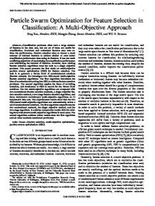
Section V concludes the study and provides possible directions for future study. II. PARTICLE SWARM OPTIMIZATION ALGORITHM PRINCIPLES The Particle Swarm Optimization PSO is a populationbased optimization method proposed by Kennedy and Eberhart [11]. The behavior of PSO can be conceivable by comparing it to school of fish searching for optimal food sources, where the direction in which a fish moves is influenced by its current movement, the best food source it ever experienced. PSO iteratively improves the accuracy of the solution to the optimization problem. Basically, optimization procedures are shown in flow chart as shown in Figure 1. These steps are described as follows:  Initialization: The n position vectors are randomly initialized {Xk (0), k = 1, 2,…, n }. The elements of Xk are uniformly distributed in a suitable range. Subsequently, the n velocity vectors {Vk (0), k = 1, 2,…, n } are randomly initialized with the elements uniformly distributed between the minimum and maximum values. The fitness of the particle is determined by the objective function [12]. The local best of each particle is initialized to its initial position and the global best to the best fitness among the best locals.



Update Position: The particle position of each particle is updated depending on the updated velocity in the following equation [14]. The updated position is based on equation (2). Xi (t+1) = Xi (t) + Vi (t+1)

(2)



Update the Local and Global Best: The fitness of each particle is evaluated based on the new updated position. If the updated position leads to a better objective function value, the local and the global best are updated.



Stopping Criteria: The three previous steps are repeated until the number of iterations is reached.

III. SELECTION SCHEMES The evolutionary algorithm (EA) is generally characterized by several features, such as a high level of population diversity. It is considered to be the best method of searching [1]. EA is discriminated in diversity population to circumvent premature convergence. A higher rate of selection from an accumulative search may lead to the loss of diversity, which in turn results in premature convergence. By contrast, if the rate of selection from the existing search is small, the search depends on randomness. Thus, the slow convergence problem may be achieved. Any selection scheme of EA consists of two main phases [15]: the selection phase, in which the selection probability is assigned to each solution in the population depending on its fitness, and the sampling phase, in which the probability controls of the sample are selected in the solutions to the next population.

Fig. 1. Flowchart of the PSO Algorithm



Update Velocity: Equation (1) updates the velocity of the particle [13]: Vi (t+1) =W.Vi (t) +C1.r1 (Pibest-Xi) + C2.r2 (Pgbest - Xi)

(1)

where C1 and C2 represent the weights of the stochastic acceleration terms to the Pibest and Pgbest

Selection schemes are classified into static and dynamic schemes [16]. The selection probability of each solution in the static selection scheme is determined in advance and then remains constant during the search. Examples of this scheme include tournament selection, linear rank, and exponential rank. By contrast, the dynamic selection scheme updates the selection probability of each solution in the population at each evolution. Another classification categorizes the selection schemes into fitness-proportionate and rank-based schemes. The fitness-proportionate class calculates the selection probability based on the absolute fitness value of each individual, whereas the selection probability in the rank-based

Page | 18

ICIT 2015 The 7th International Conference on Information Technology doi:10.15849/icit.2015.0003 © ICIT 2015 (http://icit.zuj.edu.jo/ICIT15)

class is determined based on fitness ranking rather than absolute fitness. A simple example of the fitness-proportionate scheme is the traditional proportional selection scheme. Some selection schemes have scaling problems that lead to premature convergence (e.g., proportionate selection). Other selection schemes suffer from the non-balance between fitness and the ability of reproduction (e.g., linear rank). This study focuses on modifying the PSO algorithm by amending the method of selecting the global best solution. Figure 1 shows the procedure of selecting the global best. The minimum value of the global best remains stable until the end of the iterations. In this study, each proposed selection scheme is replaced with the original selection scheme. The following subsections present some of the random selection schemes that are suggested to the method used in PSO, which can be achieved by determining the working principle for each selection method when searching for sampling and selection probability for each variable in a new PSO.

B.

Tournament selection is among the most popular selection methods in genetic algorithms. It was initially proposed by Grefenstette and Baker [18]. Algorithm (2) shows the principle of tournament selection work, which starts from the random selection of t individuals from P(t) population and then proceeds to the selection of the best individual from tournament t. This procedure is repeated n times. The best choice is frequently between two individuals, and this scheme is called binary tournament, where the choice is between t individuals called tournament size [19]. Algorithm 2. Pseudocode for the Tournament Selection Scheme 1:

A.

Proportional Selection Scheme

2:

The proportional (or roulette wheel) selection scheme proposed by Holland and John is the most traditional selection method [17]. In this method, the selection probability depends on the absolute fitness value of any solution compared with those of the other solutions in the population. The selection probability Pi for the solution i is proportional to its fitness value, which is calculated using equation (3). In Algorithm (1), r randomly picks a value uniformly from U (0, 1); sum_prob has accumulative selection probabilities, where the j

sum prob =

 P is the accumulative selection probability of i 1

solution

i

j

X . Pi 

 

f xi



swarmsize j 1

 

f xj

(3)

Algorithm 1. Pseudocode for the Proportional Selection Scheme 1: 2: 3: 4: 5: 6: 7: 8: 9: 10: 11: 12:

Set r ~ U (0, 1). Set found = false. Set sum_prob = 0. Set K = 0. While ( i ≤ swarm_size) and not (found) do sum_prob = sum_prob + Pi If (sum_prob ≥ r) then K=i found = True End If i=i+1 End While

Tournament Selection Scheme

3: 4: 5:

Choose K (the tournament size) individuals from the population at random. Choose the best individual from pool / tournament with probability P. Choose the second best individual with probability P*(1-P). Choose the third best individual with probability P*((1-P) ^2). And so on... C.

Linear Ranking Selection Scheme

Linear ranking is another selection scheme that was developed to overcome the disadvantages of the proportional selection scheme [20]. Rank selection schemes are developed to determine the selection probability of the solutions stored in PSO based on the solution fitness rank as shown in equation (4). The linear ranking selection scheme is based on the rank of individuals rather than on their fitness. Rank n is assigned to the best individual, whereas rank 1 is assigned to the worst individual. Thus, based on its rank, each individual i has the probability of being selected given by the expression [21].

Pi 

ranki  n * n  1

(4)

Once all individuals of the current population are ranked, the procedure of the linear rank selection scheme can be implemented based on Algorithm (3). D.

Exponential Ranking Selection Scheme

Exponential ranking selection sorts the probabilities of the ranked individuals by exponentially weighted as shown in

Page | 19

ICIT 2015 The 7th International Conference on Information Technology doi:10.15849/icit.2015.0003 © ICIT 2015 (http://icit.zuj.edu.jo/ICIT15)

equation (5). The main of the exponent C is situated between 0 and 1. If C 1, the difference in the selection probability between the best and the worst solutions is lost. If C 0, the difference in the selection probability becomes increasingly large and follows an exponential curve along the ranked solution. Algorithm 3. Pseudocode for Linear Ranking Selection Scheme 1: 2: 3: 4: 5: 6: 7: 8: 9: 10: 11: 12:

Set S0 = 0 For i =1 to swarm_size do Si = Si-1 + Pi End For For i =1 to swarm_size do Generate a random number r  [0,swarm_size] For each 1 ≤ j ≤ swarm_size do If ( Pj ≤ r ) do Select the jth individual End If End For. End For.

Pi 

C Ranki



swarmsize j 1

C

Rank j

(5)

Algorithm (4) for the exponential ranking, it is similar to that for the linear ranking. The only difference is in the calculation of the selection probabilities as stated in algorithm (5). IV. COMPUTATIONAL RESULTS, ANALYSIS AND DISCUSSION This section experimentally evaluates the new selection schemes. The five variations of the PSO algorithm proposed in this study are distinguished. Each variation uses a particular selection scheme that is incorporated with the PSO algorithm: 1) Global best Particle Swarm Optimization (GPSO): It uses the PSO algorithm with the global best selection scheme. 2) Proportional Particle Swarm Optimization (PPSO): It uses the PSO algorithm with the proportional selection scheme. 3) Tournament Particle Swarm Optimization (TPSO): It uses the PSO algorithm with the tournament selection scheme. 4) Linear rank Particle Swarm Optimization (LPSO): It uses the PSO algorithm with the linear rank selection scheme.

5) Exponential rank Particle Swarm Optimization (EPSO): It uses the PSO algorithm with the exponential rank selection scheme. All the experiments are conducted using a computer with processor Intel(R) Core (TM) 2 Quad CPU [email protected] GHz with 4 GB of RAM and 32-bit for Microsoft Windows 7 Professional. The source code is implemented using MATLAB (R2010a). This study applies 14 benchmarks minimization problems to compare the different selection schemes using a Algorithm 4. Pseudocode for Exponential Ranking selection scheme 1: 2: 3: 4: 5: 6: 7: 8: 9: 11: 12: 13:

Set S0 = 0 For i =1 to swarm_size do Si = Si-1 + Pi End For For i =1 to swarm_size do Generate a random number r  C For each 1 ≤ j ≤ swarm_size do If (Pj ≤ r) do Select the jth individual End If End For. End For.

large test set that involves function optimization [22]. The results of the benchmark minimization functions are used to compare the default selection schemes of PSO with the proposed selection schemes in this research. The common parameters among all the algorithms used in the experiments are set depending on the experiential instruction. The flow of the different parameter settings used to evaluate the PSO with different selection schemes is investigated. An intensive parameter analysis is conducted with various values of D, population size, C1, C2 , and W for each PSO variation as follows: dimension size D = (10, 20, and 30) [23], population size = (30, 50, and 80) [24], acceleration coefficient C1 and C2 = (1.5, 2, and 2.5) [25], and weight W = (0.5, 0.7, and 0.9) [26]. Each run is iterated 100,000 times. The best parameter setting for each variation is recorded in Table I. A series of experiments is then conducted using five convergence scenarios, each of which varies in terms of parameter settings, as shown in Table I. Each convergence scenario investigates the capability of the five parameters, and each of these parameters includes a set of values. For example the first scenario contains the GPSO with its best value of each parameter, as shown D=30, C1=1.5, C2=2, W=0.7 and pop. size= 50, These values determined as a best value for the experiments, and so on for all scenarios. A big size of dimensions requires more function evaluations. Meanwhile, increasing the computing efforts for convergence increases the reliability of the algorithm. The main point of this study is to maintain a balance between

Page | 20

ICIT 2015 The 7th International Conference on Information Technology doi:10.15849/icit.2015.0003 © ICIT 2015 (http://icit.zuj.edu.jo/ICIT15)

reliability and cost. Thus, the best value for the dimension size should be between 10 and 30 and should not be larger than 30 when the problem is complicated. The results obtained in this study are consistent with those of other researchers [4, 10, 27]. The acceleration coefficients C1 and C2 often have the same value. Based on the different empirical studies, the best value for the acceleration coefficients is C1 = C2 = C/2, where C is the total of acceleration coefficients. If C is small, then the algorithm explores slowly. [28] Kennedy suggests the same previous equation to determine C1 and C2: (C1 + C2 ≤ 4.0). The inertia weight causes a significant increase in the convergence speed and a better balance between the exploitation and exploration of the solution space, while the complexity of the algorithm increases only slightly. Therefore, the recommended inertia weight is between 0.5 and 0.9 [26]. Selecting a population size (number of particles) of 50 is recommended for higher dimensional problems, and a population size of [30, 50] is appropriate for lower dimensional problems. The values of population size are compatible with previous studies [24, 29, 30].

parameter, which means in sen5 each of the selection schemes has the best values of parameters. Each PSO variation runs 30 replications, and the numbers in the table refer to the mean and standard deviations (within the parentheses below the mean value). The best solutions are highlighted in bold (i.e., the lowest is the best). The results show that TPSO achieves the best results for all the benchmark functions. GPSO and PPSO achieve the eight best results for the Sphere, Schwefel problem 2.22, Step, Rosenbrock, Rotated hyper-ellipsoid, Rastrigin, Ackley, and Griewank benchmark functions. LPSO achieves the best results for most of the benchmark functions. By contrast, EPSO achieves poor results when compared with the other selection schemes, especially for the Rotated hyper-ellipsoid, Rastrigin, Shifted Sphere, and Shifted Rosenbrock benchmark functions. V. CONCLUSION AND FUTURE WORK This study proposed new variations of PSO based on different selection schemes. Each variation is a PSO incorporated with a selection scheme. The proposed PSO

TABLE I. PSO PARAMETERS SCENARIO Scenario No. Sen1 Sen 2 Sen 3 Sen 4 Sen 5

Selection Schemes GPSO PPSO TPSO LPSO EPSO

Parameters D

C1

C2

W

Pop. Size

30 30 30 30 30

1.5 2 2 1.5 1.5

2 2 1.5 1.5 2

0.7 0.7 0.7 0.7 0.7

50 50 30 30 50

A summary of the 14 global minimization benchmark functions used to evaluate PSO variations is presented in this study. Most of these functions were previously used in [4, 9, 31, 32]. These benchmark functions provide a trade-off between unimodal and multimodal functions. Figure 2 shows the best solutions found by the PSO variations using the 14 benchmark functions. As mentioned previously the objective form using benchmark functions is to find the minimum solution and this depend on each benchmark [33], for example in the most of a benchmark the optimal value that close to Zero. On another hand, the optimal value for some benchmark is close to (- 450) like shifted benchmark functions. This is exactly shown in figure 2, all selection schemes try to be close to the optimal solution but TPSO got the first rank on the contrary EPSO got the worst solution, PPSO, GPSO and LPSO are respectively among them. Tables II and III summarize the results of the PSO variations using the 14 benchmark functions in each convergence scenario, as shown in Table I. The results in Tables II and III are arranged from sen1 to sen5 to save the best value for each

Fig. 2. Best solutions found by the PSO variations using the 14 benchmark functions

variations - GPSO, PPSO, TPSO, LPSO, and EPSO – employed the natural selection principle of the “survival of the fittest” to generate the new PSO. These variations focused on the better solutions to the solution space. The experiments were conducted with global benchmark functions that are widely used in the literature. The experimental results show that incorporating the proposed selection scheme in the solution space by balancing exploration and exploitation prevents premature convergence and quick stagnation without efficient results. This study also produced new four selection schemes: PPSO, TPSO, LPSO, and EPSO. The experimental results show that

Page | 21

ICIT 2015 The 7th International Conference on Information Technology doi:10.15849/icit.2015.0003 © ICIT 2015 (http://icit.zuj.edu.jo/ICIT15)

these schemes perform better than GPSO. TPSO (the first position) achieves the best results, followed by PPSO and GPSO, whose results are close to each other. LPSO and EPSO are in the fourth and last positions, respectively. This study is an initial exploration of selection schemes in the PSO algorithm. Future work should analyze these selection schemes in terms of takeover time [7]. The PSO performance in other benchmark and real-life problems should be investigated as well.

Page | 22

ICIT 2015 The 7th International Conference on Information Technology doi:10.15849/icit.2015.0003 © ICIT 2015 (http://icit.zuj.edu.jo/ICIT15) TABLE II. MEAN AND STANDARD DEVIATION OF THE BENCHMARK FUNCTIONS benchmark function

Selection schemes GPSO

Sphere

PPSO TPSO LPSO EPSO GPSO PPSO

Schwefel’s problem 2.22

TPSO LPSO EPSO GPSO PPSO

Step

TPSO LPSO EPSO GPSO PPSO

Rosenbrock

TPSO LPSO EPSO GPSO PPSO

Rotated hyperellipsoid

TPSO LPSO EPSO GPSO PPSO

Schwefel’s problem 2.26

TPSO LPSO EPSO GPSO PPSO

Rastrigin

TPSO LPSO EPSO

Sen1

Sen2

Sen3

Sen4

Sen5

6.97E-06 (9.99E-06) 9.50E-06 (4.17E-06) 0.00E+00 (0.00E+00) 3.38E+04 (9.48E+03) 3.25E-01 (1.09E-01) 0.0037 (0.0025) 0.0012 (0.0012) 4.33E-25 (0.00E+00) 0.1111 (0.0842) 2.08 E+02 (3.69 E+01 ) 7.28E-05 (6.50E-05) 1.51E-06 (2.06E-06) 0.00E+00 (0.00E+00) 8.20E-03 (1.23E-02) 3.38E+02 (9.47E+02) 0.03534 (1.9019) 1.31E-06 (2.26E-06) 0.00E+00 (0.00E+00) 0.6697 (2.2043) 1.46E+03 (6.70E+02) 5.55E-05 (9.06E-05) 7.61E-06 (1.23E-05) 0.00E+00 (0.00E+00) 1.16E-03 (0.0189) 1.80E+05 (6.56E+04) -448.576769 (2.095817) -844.2568 (12.9384) -930.816247 (257.157573) -9754.924388 (399.855744) -482.3852 (773.5379) 9.69E-03 (1.72E-03) 6.85E-06 (1.30E-06) 0.00E+00 (0.00E+00) 6.69E-02 (4.83 E-02) 1.88E+04 (2.65 E+04)

4.27E-06 (2.21E-07) 8.23E-06 (2.45E-08) 6.93E-16 (2.21E-14) 4.25E-04 (3.50E-01) 3.24E-02 (2.11E-01) 0.0036 (0.0031) 5.85E-06 (0.0012) 4.57E-293 (0.00E+00) 7.35E-02 (6.84E-02) 2.07E+02 (3.81E+01) 9.50E-06 (1.20E-05) 1.51E-06 (2.06E-06) 0.00E+00 (0.00E+00) 8.20E-03 (1.99E-02) 3.19E+02 (1.00 E+02) 1.22E-04 (1.38E-04) 8.31E-05 (2.26E-05) 0.00E+00 (0.00E+00) 3.41E-01 (1.59E+00) 3.28E+02 (6.00E+02) 9.20E-05 (3.24E-05) 7.61E-06 (1.23E-05) 0.00E+00 (0.00E+00) 2.39E-03 (1.09E+00) 1.49E+02 (3.29E+05) -12564.817 (2.247382) -2517.534 (656.294850) -12567.43 (3.14213) -12561.42 (0.863088) -9765.6465 (400.078376) 6.94E-03 (9.90E-04) 6.85E-07 (1.30E-06) 0.00E+00 (0.00E+00) 1.39E-02 (1.39E-02) 1.94 E+04 (4.19 E+04)

1.47E-06 (1.92E-06) 6.58E-06 (4.25E-06) 0.00E+00 (0.00E+00) 4.80E-03 (7.30E-03) 1.56E-02 (1.88E-01) 7.99E-04 (6.65E-03) 4.76E-04 (3.77E-04) 2.57E-293 (0.00E+00) 9.76E-03 (5.90E-02) 1.004E+02 (4.259E+02) 6.21E-06 (3.57E-04) 2.07E-06 (2.72E-06) 0.00E+00 (0.00E+00) 5.69E-03 (1.59E+00) 1.46E+01 (6.00E+01) 2.55E-04 (7.69E-05) 6.58E-05 (4.25E-06) 0.00E+00 (0.00E+00) 3.85E-03 (5.21E-03) 1.52E+02 (2.11E+02) 5.55E-05 (9.06E-05) 3.651E-06 (7.32E-07) 0.00E+00 (0.00E+00) 1.04E-05 (3.40E-05) 3.24E+02 (2.11E+01) -12450.698 (2.948752) -12558.592 (9.533928) -12539.486 (0.000017) -12564.817 (2.247382) -9765.646 (400.078) 6.21E-05 (3.57E-04) 8.07E-07 (7.72E-07) 0.00E+00 (0.00E+00) 5.69E-03 (1.59E-02) 8.46E+03 (6.00E+04)

3.11E-06 (8.77E-08) 4.87E-09 (1.983E-10) 0.00E+00 (0.00E+00) 9.87E-07 (8.08E-07) 2.43E-03 (1.02E-03) 7.88E-06 (2.43E-05) 2.44E-07 (8.75E-06) 0.00E+00 (0.00E+00) 1.02E-05 (8.83E-04) 0.92E+01 (3.87E+02) 8.94E-06 (2.55E-07) 6.63E-07 (1.94E-08) 0.00E+00 (0.00E+00) 1.22E-04 (6.82E-02) 1.13E+01 (2.63E+01) 6.64E-05 (4.33E-05) 2.35E-07 (4.67E-06) 0.00E+00 (0.00E+00) 4.32E-04 (8.94E-05) 2.17 E+01 (1.49E+02) 5.69E-05 (2.44E-05) 6.84E-07 (7.56E-06) 0.00E+00 (0.00E+00) 1.56E-04 (5.21E-05) 2.33E+01 (2.83E-01) -12557.657 (2.134256) -12560.543 (2.434646) -12539.493 (1.52E-03) -12553.343 (2.854832) -9865.646 (241.532) 3.34E-06 (6.34E-05) 2.54E-07 (1.88E-07) 0.00E+00 (0.00E+00) 3.01E-03 (8.22E-02) 2.094E+03 (3.43E+03)

2.80E-07 (9.85E-08) 2.50E-06 (4.17E-06) 0.00E+00 (0.00E+00) 5.57E-07 (1.23E-08) 1.47E-06 (1.92E-06) 8.43E-07 (1.12E-09) 9.23E-09 (4.65E-08) 0.00E+00 (0.00E+00) 5.23E-06 (3.87E-06) 0.69E+02 (0.54E+02) 1.75E-08 (2.54E-07) 8.78E-10 (6.59E-09) 0.00E+00 (0.00E+00) 4.98E-06 (2.73E-06) 2.39E+00 (2.31E+00) 1.65E-06 (2.37E-07) 3.08E-07 (6.29E-06) 0.00E+00 (0.00E+00) 2.82E-07 (7.65E-06) 1.06 E+01 (2.00E+02) 5.59E-06 (2.39E-06) 5.69E-08 (3.49E-09) 0.00E+00 (0.00E+00) 3.85E-07 (5.21E-05) 6.94 E+00 (1.06E+01) -12559.293 (2.267349) -12563.685 (1.950643) -12563.978 (1.08E-03) -12566.854 (1.098576) -11783.543 (223.495) 1.59E-06 (3.94E-06) 4.58E-08 (4.59E-07) 0.00E+00 (0.00E+00) 4.45E-04 (2.15E-03) 7.69E+01 (2.05E+01)

Page | 23

ICIT 2015 The 7th International Conference on Information Technology doi:10.15849/icit.2015.0003 © ICIT 2015 (http://icit.zuj.edu.jo/ICIT15) TABLE III. MEAN AND STANDARD DEVIATION OF THE BENCHMARK FUNCTIONS benchmark function

Selection schemes GPSO PPSO

Ackley

TPSO LPSO EPSO GPSO PPSO

Griewank

TPSO LPSO EPSO GPSO PPSO

Camel-Back

TPSO LPSO EPSO GPSO PPSO

Shifted Sphere

TPSO LPSO EPSO GPSO PPSO

Shifted Schwefel’s problem 1.2

TPSO LPSO EPSO GPSO PPSO

Shifted Rosenbrock

TPSO LPSO EPSO GPSO PPSO

Shifted Rastrigin

TPSO LPSO EPSO

Sen1

Sen2

Sen3

Sen4

Sen5

5.65E-02 (4.26E-02) 9.37E-03 (2.70E-02) 4.88E-03 (0.00E+00) 7.2318 (5.2197) 19.6590 (2.8761) 6.35E-04 (1.38E-05) 2.38E-05 (5.89E-05) 0.00E+00 (0.00E+00) 0.0563 (0.0832) 1.34E+02 (1.76E+02) -0.9275 (0.097) -0.7673 (0.2075) -0.7356 (0.00E+00) 0.7389 (2.2041) 7.22E+02 (8.28E+02) 1.74E+03 (6.20E+02) 1.85E+03 (6.10E+02) 2.64E+03 (1.03E+03) 3.27E+04 (8.94E+03) 1.94E+05 (4.90E+05) 5.41E+03 (1.26E+03) 5.04E+03 (1.39E+03) 7.98E+03 (3.35E+03) 1.87E+05 (9.08E+04) 5.71E+03 (1.50E+03) 2.12E+11 (2.24E+10) 2.14E+11 (2.60E+10) 2.49E+11 (6.54E+10) 2.17E+12 (6.42E+11) 2.14E+11 (2.60E+10) 143.079 (26.8865) 143.0297 (21.7146) 143.6271 (17.9028) 8.79E+02 (172.0375) 923.7594 (47.333)

2.46E-02 (5.34E-02) 5.58E-04 (7.85E-04) 0.00E+00 (0.00E+00) 4.5235 (7.67E-01) 18.2253 ( 0.792) 2.38E-04 (5.89E-04) 5.80E-06 (7.44E-04) 0.00E+00 (0.00E+00) 6.06E-02 (6.09E-03) 4.96E+01 (6.65E+01) -8.98E-01 (3.24E-01) -7.98E-01 (5.012E-01) -5.34E-01 (3.12E-01) 1.53E+00 (3.63E+00) 9.34E+02 (1.05E+03) 5801.689232 (1761.064344) -445.9264 (0.028288) -449.999836 (0.008747) 5801.689232 (1761.064344) 5.80 E+04 (3.76 E+05) 946598.695 (309138.764) -48.748413 (366.028440) -447.007381 (2.969228) -449.933552 (0.052206) 6598.695551 (9138.764095) 515.19 (105.6652) 497.01 (106.87) 486.825 (120.596) 589.40 (309.94) 1506.80 (1.87 E+7) -329.8838 (0.304559) -329.951 (0.184239) -220.091 (13.0087) -329.951 (0.184239) 1026.852 (1876.38)

1.01E-02 (6.54 E-03) 1.14E-04 (2.75E-04) 0.00E+00 (0.00E+00) 3.4935 (2.26E-02) 18.2455 (7.29E-01) 1.65E-05 (7.08E-05) 5.80E-06 (7.44E-04) 0.00E+00 (0.00E+00) 7.03E-04 (1.86E-03) 3.87E+01 (2.97E+01) -9.18E-01 (4.84E-01) -9.44E-01 (9.873E-01) -9.79E-01 (7.02E-03) 1.01E+00 (1.03E+02) 5.86E+02 (9.74E+01) 287.280860 (2085.974382) -447.6589 (0.757310) -447.999877 (0.000943) 3565.63289 (1076.69087) 2.57 E+04 (2.08 E+05) -439.933552 (0.052206) -449.668252 (366.028440) -449.75496 (6.474446) -216.64485 (0.052206) 2643.859146 (7586.125628) 509.54320 (363.352) 498.744 (116614) 495.595 (123.986) 597.585 (109.454) 1122.625 (1.56 E+6) -329.235 (0.848076) -429.768 (0.184239) -328.534 (2.87987) -389.098 (1.760988) 1751.450 (1555.89)

7.66E-03 (2.38E-04) 8.12E-04 (3.55E-05) 0.00E+00 (0.00E+00) 0.6697 (1.00E-02) 17.4673 (3.32E-03) 3.23E-07 (8.63E-06) 6.85E-07 (8.30E-06) 0.00E+00 (0.00E+00) 1.25E-05 (7.43E-04) 3.02E+01 (2.97E+01) -9.01E-01 (3.94E-01) -9.95E-01 (9.86E-01) -9.79E-01 (7.02E-03) 1.01E+00 (1.03E+02) 5.86E+02 (9.74E+01) -440.856 (2.642622) -442.789 (1.45624) -448.543 (1.43676) 753.538 (7.33E+04) 9.56 E+03 (6.58E+04) -440.863 (1.9564) -441.698 (1.32E-01) -448.365 (1.38E-02) -421.302 (8.29E-02) 4085.025 (3878.464) 501.3213 (206.653) 469.005 (2.86E+02) 421.203 (332.845) 578.230 (283.865) 983.748 (1.72E+04) -302.738 (0.304559) -320.765 (1.54677) -329.654 (4.51E-02) -289.765 (0.3472) -201.543 (39.6543)

6.45E-04 (9.32E-04) 3.43E-06 (8.56E-07) 0.00E+00 (0.00E+00 0.2849 (6.66E-3) 13.9837 (1.27E-03) 4.54E-07 (7.35E-06) 7.26E-08 (5.68E-08) 0.00E+00 (0.00E+00) 1.02E-06 (2.45E-04) 2.11E+00 (1.02E+00) -8.67E-01 (3.26E-01) -9.21E-01 (2.02E-01) -9.98E-01 (9.87E-03) -8.98E-01 (1.75E-02) 3.87E+01 (9.74E-01) -448.624 (1.364865) -449.086 (2.456782) -449.958 (0.076328) 742.756 (2.39E+04) 6.32 E+03 (6.65E+03) -449.661 (0.07654) -449.827 (2.69E-02) -449.947 (7.09E-02) -439.546 (6.67E-02) 546.131 (558.315) 502.1478 (302.579) 465.744 (2.00E+02) 388.564 (203.432) 554.587 (229.545) 876.432 (1.65E+04) -319.454 (0.54786) -323.564 (0.342) -429.654 (3.69E-02) -320.969 (0.7649) -281.203 (4.875)

Page | 24

ICIT 2015 The 7th International Conference on Information Technology doi:10.15849/icit.2015.0003 © ICIT 2015 (http://icit.zuj.edu.jo/ICIT15)

REFERENCES [1]

[2] [3] [4] [5]

[6]

[7] [8]

[9]

[10]

[11]

[12]

[13]

[14]

[15]

[16] [17]

Z. Cui, and X. Gao, “Theory and applications of swarm intelligence,” Neural Computing and Applications, vol. 21, no. 2, pp. 205-206, 2012. M. Rabinovich, P. Kainga, D. Johnson et al., "Particle swarm optimization on a gpu." pp. 1-6, 2012. R. C. Eberhart, and J. Kennedy, "A new optimizer using particle swarm theory." pp. 39-43, 1995. Y. Shi, and R. C. Eberhart, "Empirical study of particle swarm optimization", 1999. X. Wu, Q. Xu, L. Xu et al., “Genetic white matter fiber tractography with global optimization,” Journal of neuroscience methods, vol. 184, no. 2, pp. 375-379, 2009. R. Poli, J. Kennedy, and T. Blackwell, “Particle swarm optimization,” Swarm intelligence, vol. 1, no. 1, pp. 33-57, 2007. Y. Shi, and R. Eberhart, "A modified particle swarm optimizer." pp. 69-73, 1998. N. Lynn, and P. N. Suganthan, "Distance Based Locally Informed Particle Swarm Optimizer with Dynamic Population Size." pp. 577-587, 2015. R. C. Eberhart, and Y. Shi, "Comparing inertia weights and constriction factors in particle swarm optimization." pp. 84-88, 2000. R. C. Eberhart, and Y. Shi, "Particle swarm optimization: developments, applications and resources." pp. 81-86, 2001. S. Sen, P. Roy, and S. Sengupta, “Regular paper AI based Break-even Spot Pricing and Optimal Participation of Generators in Deregulated Power Market,” J. Electrical Systems, vol. 8, no. 2, pp. 226235, 2012. M. A. Mohandes, “Modeling global solar radiation using Particle Swarm Optimization (PSO),” Solar Energy, vol. 86, no. 11, pp. 3137-3145, 2012. E. Zahara, and Y.-T. Kao, “Hybrid Nelder–Mead simplex search and particle swarm optimization for constrained engineering design problems,” Expert Systems with Applications, vol. 36, no. 2, pp. 38803886, 2009. C.-F. Juang, “A hybrid of genetic algorithm and particle swarm optimization for recurrent network design,” Systems, Man, and Cybernetics, Part B: Cybernetics, IEEE Transactions on, vol. 34, no. 2, pp. 997-1006, 2004. M. A. Al-Betar, I. A. Doush, A. T. Khader et al., “Novel selection schemes for harmony search,” Applied Mathematics and Computation, vol. 218, no. 10, pp. 6095-6117, 2012. T. Back, “ Evolutionary algorithms in theory and practice. ” Oxford Univ. Press, 1996. J. H. Holland, “ Adaptation in natural and artificial systems. ” An introductory analysis with applications to biology, control, and artificial intelligence: U Michigan Press, 1975.

[18]

[19] [20]

[21]

[22]

[23]

[24] [25]

[26] [27]

[28] [29]

[30]

[31]

[32]

[33]

J. J. Grefenstette, and J. E. Baker, "How genetic algorithms work: A critical look at implicit parallelism." pp. 20-27, 1989. T. Blickle, and L. Thiele, "A Mathematical Analysis of Tournament Selection." pp. 9-16, 1995. L. D. Whitley, "The GENITOR Algorithm and Selection Pressure: Why Rank-Based Allocation of Reproductive Trials is Best." pp. 116-123, 1989. T. Blickle, and L. Thiele, “A comparison of selection schemes used in evolutionary algorithms,” Evolutionary Computation, vol. 4, no. 4, pp. 361-394, 1996. V. S. Gordon, and D. Whitley, "Serial and parallel genetic algorithms as function optimizers." pp. 177183, 1993. I. C. Trelea, “The particle swarm optimization algorithm: convergence analysis and parameter selection,” Information processing letters, vol. 85, no. 6, pp. 317-325, 2003. M. Richards, and D. Ventura, "Dynamic sociometry in particle swarm optimization." pp. 1557-1560, 2003. U. KC, T. Deconinck, P. Varghese et al., "Experimental and numerical studies of a direct current microdischarge plasma thruster." pp. 585-600, 2001. Y. Shi, and R. C. Eberhart, "Fuzzy adaptive particle swarm optimization." pp. 101-106, 2001. X. Jin, Y. Liang, D. Tian et al., “Particle swarm optimization using dimension selection methods,” Applied Mathematics and Computation, vol. 219, no. 10, pp. 5185-5197, 2013. J. Kennedy, "The behavior of particles." pp. 579-589, 1998. Z. Li-Ping, Y. Huan-Jun, and H. Shang-Xu, “Optimal choice of parameters for particle swarm optimization,” Journal of Zhejiang University Science A, vol. 6, no. 6, pp. 528-534, 2005. X. Hu, and R. Eberhart, "Solving constrained nonlinear optimization problems with particle swarm optimization." pp. 203-206, 2002. J. J. Liang, A. K. Qin, P. N. Suganthan et al., “Comprehensive learning particle swarm optimizer for global optimization of multimodal functions,” Evolutionary Computation, IEEE Transactions on, vol. 10, no. 3, pp. 281-295, 2006. P. Civicioglu, and E. Besdok, “A conceptual comparison of the Cuckoo-search, particle swarm optimization, differential evolution and artificial bee colony algorithms,” Artificial Intelligence Review, vol. 39, no. 4, pp. 315-346, 2013. J. Vesterstrom, and R. Thomsen, "A comparative study of differential evolution, particle swarm optimization, and evolutionary algorithms on numerical benchmark problems." pp. 1980-1987, 2004.

Page | 25