ignore topological features of the nodes and are used in combination with the ... wireless sensor networks, based on a novel metric for characterizing the ...
Node Clustering in Wireless Sensor Networks by Considering Structural Characteristics of the Network Graph∗ Nikos Dimokas1 1 2
Dimitrios Katsaros1,2
Yannis Manolopoulos1
Department of Informatics, Aristotle University, Thessaloniki, Greece
Department of Computer & Communication Engineering, University of Thessaly, Volos, Greece {dimokas,dimitris,manolopo}@delab.csd.auth.gr http://delab.csd.auth.gr/∼ {dimokas,dimitris,manolopo}
Abstract The deployment of wireless sensor networks in many application areas, e.g., aggregation services, requires self-organization of the network nodes into clusters. Quite a lot of node clustering techniques have appeared in the literature, and roughly fall into two families; those based on the construction of a dominating set and those which are based solely on energy considerations. The former family suffers from the fact that only a small subset of the network nodes are responsible for relaying the messages, and thus cause rapid consumption of the energy of these nodes. The later family uses the residual energy of each node in order to direct its decision about whether it will elect itself as a leader of a cluster or not. This family’s methods ignore topological features of the nodes and are used in combination with the methods of the former family. We propose a novel distributed clustering protocol for wireless sensor networks, based on a novel metric for characterizing the importance of a node, w.r.t. its contribution in relaying messages. The protocol achieves small communication complexity and linear computation complexity. Experimental results for various sensor network topologies show that the protocol generates only a few clusters, guaranteeing a small number of message relays thus improving network lifetime. Keywords. Sensor networks, clustering, network lifetime, energy conservation, backbone formation.
1
Introduction
The rapid technological advances in the fields of antennas, radio, transceivers and processors with respect to their form, size, power efficiency and the ∗ Research supported by a ΓΓET grant in the context of the project “Data Management in Mobile Ad Hoc Networks” funded by ΠYΘAΓOPAΣ II national research program.
progress in the area of microsensors, have fueled a new research and development arena, that of wireless sensor networks. A wireless sensor network (WSN) is a collection of tiny sensors, each being capable of “sensing/monitoring” the environment, processing these sensed “signals” and communicating (transmitting and receiving) with other sensor nodes. Communication in a WSN between any two nodes that are out of one another’s transmission range is achieved through intermediate nodes, which relay messages to set up a communication channel between the two nodes. In many applications, the sensor nodes are left unattended to continuously report their measurements until they run out of energy (battery). There are many application areas benefited from WSN, e.g., habitat monitoring [16], disaster relief [17], target tracking [5] and so on. Many of these applications require simply an aggregate value to be reported to the “information sink” (observer, base station, etc.). In these cases, sensors in different regions of the field can collaborate to aggregate the information they gathered. For instance, in habitat monitoring applications the sink may require the average of temperature; in military applications the existence or not of high levels of radiation may be the target information that is being sought. It is evident that by organizing the sensor nodes in groups i.e., clusters of nodes, we can reap significant network performance gains. Clustering not only allows aggregation, but limits data transmission primarily within the cluster, thereby reducing both the network traffic and the contention for the channel. The clustering procedure starts with the discovery of neighboring sensor nodes (SN) by sending periodic Beacon Signals. After the creation of the clusters, each cluster is coordinated by the cluster head (CH) node, which is responsible for getting the measured values from its cluster’s nodes and then aggregate them, be-
fore send the aggregates to the sink(s) through other CHs. Several studies [9, 19] indicate that clustering increases the network lifetime. Although the definition of the network lifetime depends on the applications’ semantics, a widely accepted definition is the time until the first/last node of the network depletes its energy [20]. Apart from clustering, there exist also other strategies to increase network lifetime, like indexing [10, 12], but these are orthogonal to clustering. The issue of network node clustering first appeared in [2], reconsidered in [8, 11], and later improved in [1, 3, 6, 13, 15, 18] in the context of mobile ad hoc networks. All these efforts recognized the significance of selecting the most “appropriate” nodes as cluster heads and they did this through the use of the notion of dominating sets (DS), i.e., a subset of the network nodes such that any node of the network graph either belongs to the DS or is a neighbor of a node of the DS. A survey of this type of methods can be found in [4]. The major shortcoming of this type of algorithms is the fact that the nodes belonging to the DS are solely responsible for carrying out all communication, thus running out of energy very soon. Apart from this family of algorithms, a second family provided mechanisms to address the energy consumption problem due to the repetitive communication by the same nodes, i.e., the cluster heads. This family of protocols essentially proposed ways to “rotate” the role of cluster-head among nodes of clusters, e.g., the SPAN [7], the LEACH [9], the HEED [19] protocols and they can be coupled with the algorithms of the first family. They are not usually characterized as clustering techniques and thus we strive to improve the first family of algorithms. The techniques of the second family can be easily incorporated/combined. All clustering algorithms proposed so far (see [4, 20] for more complete surveys), present some weaknesses. Some methods rely on node IDs in eliminating potential redundant broadcasting nodes or in defining priorities, e.g., [1, 3, 6, 15, 18]. These approaches suffer from the fact that they can not detect all possible eliminations, because ordering based on node id (or node weight) prevents this. As a consequence they incur significantly excessive retransmissions. Some methods (e.g., [2, 8, 11, 13, 15]) do not fully exploit the compiled information; for instance, the use of the node degree as its priority when deciding whether it will become a cluster head might not result in the best local decision. Finally, some methods create a lot of clusters [18], or require excessive communication cost [1]. Here, we propose a novel clustering protocol for wireless sensor networks, which complies with all requirements described in [20]:
• it is localized, thus distributed; it can exploit 1hop, 2-hop or k-hop neighborhood information, presenting different tradeoffs in efficiency vs. communication cost, but for the sake of readability we present it here assuming knowledge of the 2-hop neighborhood of a sensor node, • the cluster heads are estimated dynamically depending on the originator node, which wishes to transmit a message, thus the cluster heads are not static avoiding fast depletion of their energy, • introduces a novel measure for capturing a node’s significance/presence w.r.t. the fact that the node resides in networks paths that will definitely be traversed by the majority of the transmitted messages, • computes a node’s significance in time linear in the number of nodes and linear in the number of edges of the network neighborhood of the node, irrespectively of the degree of each node, • allows for fast network clustering, thus (in combination with the aforementioned feature) is appropriate for reclustering operations. The rest of the paper is organized as follows: In Section 2 we describe a novel metric for measuring sensor nodes’ significance and the respective clustering protocol built upon this metric. In Section 3, we evaluate through simulation the proposed protocol, and finally in Section 4 we conclude the paper.
2 2.1
The new sensor node clustering protocol Preliminaries
Before proceeding in the presentation of the main paper ideas, we will give some necessary definitions. A wireless sensor network is abstracted as a graph G(V, E). An edge e = (u, v), u, v ∈ E exists if and only if u is in the transmission range of v and vice versa. All links in the graph are bidirectional. The set of neighbors of a node v is represented by N1 (v), i.e., N1 (v) = {u : (v, u) ∈ E}. The set of two-hop nodes of node v, i.e., the nodes which are the neighbors of node v’s neighbors except for the nodes that are the neighbors of node v, is represented by N2 (v), i.e., N2 (v) = {w : (u, w) ∈ E, where w �= v and w ∈ / N1 and (v, u) ∈ E}. The combined set of one-hop and two-hop neighbors of v is denoted as N12 (v). Definition 1 (Local network view w.r.t. node v) The local network view, denoted as LNv , of a graph G(V, E) w.r.t. a node v ∈ V is the induced subgraph of G associated with the set of vertices in N12 (v).
We define a path from u ∈ V to w ∈ V as an alternating sequence of vertices and edges, beginning with u and ending with w, such that each edge connects its preceding with its succeeding vertex. The length of a path is the number of intervening edges. We denote by dG (u, w) the distance between u and w, i.e., the minimum length of any path connecting u and w in G, where by definition dG (v, v) = 0, ∀v ∈ V and dG (u, w) = dG (w, u), ∀u, w ∈ V . Note that the distance is not related to network link costs (e.g., latency), but it is a purely abstract metric measuring the number of hops.
2.2
Measuring node significance
We mentioned in the introduction that all methods to-date use the node id or the node’s degree in prioritizing the node for inclusion in the dominating set, e.g., [13, 15]. Some methods first consider the node(s) which serves as the only neighbor of a node in N12 (·) and then examine the node(s) with the maximum degree w.r.t. nodes not covered yet, whereas other methods simply consider the node(s) with the highest degree. None of these approaches is appropriate because: a) the former methods treat nodes in a heterogeneous way, and b) later methods, even though they are aware of the 2hop neighborhood, do not make full usage of the available information. In the sequel, we will present a new definition of node’s significance that avoids both drawbacks. Let σuw = σwu denote the number of shortest paths from u ∈ V to w ∈ V (by definition, σuu = 0 ). Let σuw (v) denote the number of shortest paths from u to w that some vertex v ∈ V lies on. Then, we define the node importance index N I(v) of a vertex v as: Definition 2 The node importance index N I(v) of a vertex v is equal to: N I(v) =
� u�=v�=w∈V
σuw (v) . σuw
X (0) Y (0)
A (6.67)
T (1.33)
U (54)
P (41)
Z (0)
V (1.33) B (13) W (3.33) Q (8) R (9.33)
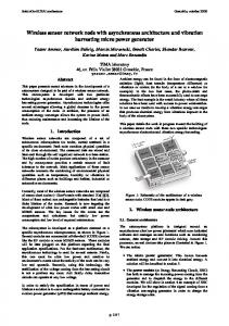
Figure 1. Calculation of N I for a sample graph. Each node is characterized by a pair of ID(N I).
the network, i.e., nodes that act as articulation points, or nodes with large degree relative to their neighbors. In this sense, it can be proved that N I generalizes the concept of node degree, as this has been used for clustering purposes so far. The N I index would be useful in designing clustering protocols in sensor networks only if it captures structural features of small graphs, e.g., of the 2-hop neighborhood of a node and only if it can be computed really fast. If these conditions hold, then it can be used in designing localized algorithms. Indeed, they both hold. The reader can easily verify that, for any node v, the N I indexes of the nodes in N12 (v) calculated only for the subgraph LNv reveal the relative importance of the nodes in covering the subgraph N12 (from v’s point of view). For instance, the N I index for the nodes belonging to LNP (see Figure 1) are indicated in Table 1. For a node u, which belongs to the 2-hop neighborhood of a node v (or if u ≡ v), the N I index of u (calculated over LNv ) will be denoted as N I v (u). n(ode)
X T V W
N I P (n) 0 0 0 0
n(ode)
Y U R P
N I P (n) 0 81.67 6 44.33
n(ode) N I P (n)
Q A B Z
6.33 7 12.67 0
Table 1. N I index of the nodes belonging to LNP . (1)
Large values for the N I index of a node v indicate that this node v can reach others on relatively short paths, or that the node v lies on considerable fractions of shortest paths connecting others. Let us see the N I indexes for the nodes of the graph presented in Figure 1 of [15]. The results are illustrated in our Figure 1. We observe that the N I index calculated over the whole graph captures structural features of the graph better than the node degree does. Moreover, it induces a ranking of the nodes according to their contribution in covering the whole network. Actually, the N I value identifies what we would call the geodesic nodes of
At a first glance, the computation of the N I seems expensive, i.e., O(m∗n2 ) operations in total for a 2-hop neighborhood, which consists of n nodes and m links. Fortunately, we can do better than this by making some smart observations. For the interest of space, we will not present the details here, but direct the readers to the Appendix A, where we present the pseudo-code of the algorithm ComputeNI for the calculation of the N I index of a node. The algorithm is capable of handling multiple shortest paths between two nodes, that is why some node have fractional N I. Theorem 1 The algorithm ComputeNI is correct in the sense that, when it executes (on a whole network
or a neighborhood), it correctly calculates the number of shortest paths passing through a node (of this network or the neighborhood). Theorem 2 The complexity of the algorithm ComputeNI is O(n ∗ m) for a graph with n vertices and m edges.
2.3
The clustering protocol
The individual procedures for the creation of the clusters are not radically different from those developed for other clustering protocols [3, 4, 8, 11, 15]. Thus for the interest of space, we will not proceed in the detailed description of these procedures, but instead we assume that the reader is familiar with them. We assume a sensor network in which the nodes periodically exchange with their neighbors “Hello” messages (beacon signals), which contain the list of their one hop neighbors. (Recall that the protocol works unchanged also in the case that the nodes simply notify for their existence, without informing about their neighbors). Thus, each node is able to form a graph that corresponds to its 2-hop neighborhood (or its 1-hop neighborhood). Also, each node, when it receives a packet, is able to figure out from which 1-hop neighbor this packet was sent. The proposed clustering protocol is dynamic or source-dependent, i.e., the elected cluster heads depend on the location of the source and the progress of the clustering process, avoiding thus the effect of the “hotspots”. We name the protocol as GESC, from the initials of the words GEodegic Sensor Clustering protocol. Theorem 3 The GESC algorithm is reliable, in the sense that the broadcasted packet can be disseminated to every node in the network (if it is connected).
3
Performance Evaluation
We conducted several experiments to evaluate the performance of our algorithm and compare it to other protocols. We examined the most efficient algorithms reported in [4, 20], and thus we compare GESC to MPR [13], WL [18] and with SSZ [15], which was selected as a Fast Breaking Paper in Computer Science for October 2003. As performance metrics, we measure the energy dissipation, broadcast messages, and latency. All the protocols have been implemented using the J-Sim simulation library [14]. We tested the protocols for a variety of sensor network topologies with 100, 300 and 500 nodes, to simulate sensor networks with varying levels of node degree, from 4 to 10. Each topology consists of many square grid units where one or more nodes are placed. The
number of square grid units depends on the number of nodes and on the node degree. The topologies are generated as follows: the location of each of the n sensor nodes is uniformly distributed between the point (x = 0, y = 0) and the point (x = 100, y = 100). The average degree d is computed by sorting all n∗(n−1)/2 edges in the network by their length, in increasing order. The grid unit size corresponding to the value of d is equal to 23 times the length of the edge at position n∗d 2 in the sorted sequence. Two sensor nodes are neighbors if they are placed in the same grid or in adjacent grid units. We tested each topology over an 100X100m2 sensor field divided into grids. The network is generated as above with the precondition that it is connected and the sensor nodes are static. Each node is assigned a unique id and x, y coordinates within the simulation area. We used the energy model available by J-Sim. We run each protocol at least 100 times for each different node degree, before computing the averages of the number of broadcast messages diffused into the network and the average of consumed energy. In each run, a different node is selected to start the broadcasting process.
3.1
Evaluation
Impact of the number of nodes. The first experiment evaluated the impact of the number of nodes of the sensor network on the number of messages generated during cluster formation (Figure 2) and during broadcasting procedures (Figure 3). We can easily figure out the linear dependence of the number of transmitted messages on the network size and the efficiency of the GESC protocol for the broadcasting procedure, since it generates few cluster and thus cluster heads, which are responsible for forwarding any messages. GESC always performs from 4% to 10% better than the second best performing algorithm (SSZ) no matter what the scale of the network is (in terms of number of nodes). It is worthy to notice that all methods generate the same number of messages during cluster formation, since they all have to learn their immediate (1-hop or 2-hop) neighbors, and apparently this number does not depend on the connectivity (average degree) of the network. On the other hand, the average degree has beneficial effect on the broadcasting procedure, since allows for faster message dissemination; in such settigns the performance gap between GESC and the competing algorithms widens. Impact of the average node degree. The second experiment evaluated the impact of the average node degree on the number of messages generated during cluster formation (left part of Figure 4) and during
cluster formation cost
cluster formation cost
average broadcast procedure cost
600
2000
170
1800
1200 1000 800 600
WL MPR SSZ GESC
500
number of messages
1400
450
400
350
0 100
300
300
400
500 600 700 number of nodes cluster formation cost
800
900
number of messages
120
5
6
7 8 average degree
9
10
4
5
6
7 8 average degree
9
10
Figure 4. Impact of the average node degree on cluster formation (left) and on the number of transmissions (right) for a network of 300 sensor nodes.
1800
1400
130
1000
2000
1600
140
100 4
200
150
110
400 200
WL MPR SSZ GESC
160
550
WL MPR SSZ GESC
number of messages
number of messages
1600
WL MPR SSZ GESC
1200 1000 800 600 400 200 0 100
200
300
400
500 600 700 number of nodes
800
900
1000
Figure 2. Impact of the nodes’ number on cluster formation for degree equal to 4 (top) and for degree equal to 10 (bottom).
tion. We examined the residual energy of each sensor node after all experimental tests and draw plots depicting it. Here, we present only a characteristic case (Figure 5). We can easily observe the “energy starvation” that SSZ and MPR cause in some nodes, whereas GESC achieves to maintain more balancing in the energy of the nodes. 10 WL MPR SSZ GESC
average broadcast procedure cost 600
9.5
400
WL MPR SSZ GESC
9
300
Residual Energy
number of messages
500
200
100
0 100
200
300
400
500 600 700 800 number of nodes average broadcast procedure cost
900
8.5
8
7.5
1000
7
500
6.5
450
number of messages
400 350
WL MPR SSZ GESC
6 0
20
300
40
60
80
100
Individual Nodes
250
Figure 5. Plot of the residual energy for a topology of 100 nodes.
200 150 100 50 0 100
200
300
400
500 600 700 number of nodes
800
900
1000
Figure 3. Impact of the nodes’ number on transmission for degree equal to 4 (top) and for degree equal to 10 (bottom).
the broadcasting procedure (right part of Figure 4). We present a selection of the results concerning a sensor network with 300 nodes. Again, GESC is the best performing algorithm, with gains up to 20% relative to the second best performing method. For small node degrees, their performance is almost equivalent, but with larger degrees the performance of GESC gets steadily better than SSZ’s. Impact on the energy consumption. Our last experiment investigated the issue of energy consump-
4
Conclusions
We introduced a new distributed clustering protocol for wireless sensor networks, the GESC protocol. The proposed protocol is based on a novel localized metric for measuring the value of a node in “covering” the neighborhood with its rebroadcast. The calculation of this metric is linear in the number of nodes and linear in the number of radio links, thus appropriate for frequent reclustering operations. With J-Sim simulator, we tested the protocol’s performance and the results obtained attest that the proposed protocol is very efficient and it is able to reap significance performance gains in terms of communication cost (few transmitted messages) and also in terms of network longevity (reasonably balancing the energy of the nodes).
References [1] A. D. Amis, R. Prakash, T. H. P. Vuong, and D. T. Huynh. Max-min d-cluster formation in wireless ad hoc networks. In Proceedings of the Annual Joint Conference of the IEEE Computer and Communications Societies (INFOCOM), volume 1, pages 32–41, 2000. [2] D. Baker and A. Ephremides. The architectural organization of a mobile radio network via a distributed algorithm. IEEE Transactions on Communications, 29(11):1694–1701, 1981. [3] S. Basagni. Distributed clustering for ad hoc networks. In Proceedings of the International Symposium on Parallel Architectures, Algorithms and Networks (ISPAN), pages 310–315, 1999. [4] S. Basagni, M. Mastrogiovanni, A. Panconesi, and C. Petrioli. Localized protocols for ad hoc clustering and backbone formation: A performance comparison. IEEE Transactions on Parallel and Distributed Systems, 17(4):292–306, 2006. [5] P. K. Biswas and S. Phoha. Self-organizing sensor networks for integrated target surveillance. IEEE Transactions on Computers, 55(8):1033–1047, 2006. [6] M. Chatterjee, S. Das, and D. Turgut. WCA: A weighted clustering algorithm for mobile ad hoc networks. ACM/Kluwer Cluster Computing, 5(2):193– 204, 2002. [7] B. Chen, K. Jamieson, H. Balakrishnan, and R. Morris. SPAN: An energy efficient coordination algorithm for topology maintenance in ad hoc networks. ACM/Kluwer Wireless Nerworks, 8(5):481–494, 2002. [8] M. Gerla and J.-C. Tsai. Multicluster, mobile, multimedia radio network. ACM/Baltzer Wireless Networks, 1(3):255–265, 1995. [9] W. B. Heinzelman, A. P. Chandrakasan, and H. Balakrishnan. An application-specific protocol architecture for wireless microsensor networks. IEEE Transactions on Wireless Communications, 1(4):660–670, 2002. [10] D. Katsaros, N. Dimokas, and Y. Manolopoulos. Generalized indexing for energy-efficient access to partially ordered broadcast data in wireless networks. In Proceedings of the IEEE International Database Engineering and Applications Symposium (IDEAS), 2006. [11] C. R. Lin and M. Gerla. Adaptive clustering for mobile wireless networks. IEEE Journal on Selected Areas in Communications, 15(7):1265–1275, 1997. [12] A. Meka and A. K. Singh. DIST: A distributed spatio-temporal index structure for sensor networks. In Proceedings of the ACM Conference on Information and Knowledge Management (CIKM), pages 139–146, 2005. [13] A. Qayyum, L. Viennot, and A. Laouiti. Multipoint relaying: An efficient technique for flooding in mobile wireless networks. Technical Report 3898, INRIA, March 2000. [14] A. Sobeih, J. C. Hou, L.-C. Kung, N. Li, H. Zhang, W.-P. Chen, H.-Y. Tyan, and H. Lim. J-Sim: A simulation and emulation environment for wireless sensor networks. IEEE Wireless Communications magazine, 13(4):104–119, 2006.
[15] I. Stojmenovic, M. Seddigh, and J. Zunic. Dominating sets and neighbor elimination-based broadcasting algorithms in wireless networks. IEEE Transactions on Parallel and Distributed Systems, 13(1):14–25, 2002. [16] R. Szewczyk, E. Osterweil, J. Polastre, M. Hamilton, A. Mainwaring, and D. Estrin. Habitat monitoring with sensor networks. Communications of the ACM, 47(6):34–40, 2004. [17] Y.-C. Tseng, M.-S. Pan, and Y.-Y. Tsai. Wireless sensor networks for emergency navigation. IEEE Computer, 39(7):55–62, Aug. 2006. [18] J. Wu and H. Li. A dominating-set-based routing scheme in ad hoc wireless networks. Telecommunication Systems, 18(1–3):13–36, 2001. [19] O. Younis and S. Fahmy. HEED: A hybrid, energyefficient, distributed clustering approach for ad hoc sensor networks. IEEE Transactions on Mobile Computing, 3(4):366–379, 2004. [20] O. Younis, M. Krunz, and S. Ramasubramanian. Node clustering in wireless sensor networks: Recent developments and deployment challenges. IEEE Network, 20(3):20–25, May/Jun. 2006.
A
Computation of the NI
Algorithm ComputeNI (graph G(N, L)) // N : set of graph nodes, L: set of links between these nodes // Output: Array N I[·]: N I index value for each node of N
begin N I[t] = 0, ∀t ∈ N ; foreach( n ∈ N ) do { S: an empty stack; P [·]: array of empty lists (one list ∀ node w ∈ N ); σ[·]: an array, where σ[t] = 0, ∀t ∈ N ; σ[n]=1; d[·]: an array, where d[t] = −1, ∀t ∈ N ; d[n]=0; Q: an empty queue; Q.enqueue(n); while( Q.isN otEmpty() ){ v = Q.dequeue(); S.push(v); foreach 1-hop neighbor w of v do // w found for the first time?
if( d[w] < 0 ) then Q.enqueue(w); d[w] = d[v] + 1; // shortest path to w via v?
if( d[w] == (d[v] + 1) ) then σ[w] = σ[w] + σ[v]; P [w].append(v);
} δ[·]: an array, where δ[t] = 0, ∀t ∈ N ;
// S returns nodes in order of non-increasing hop distance from n
while( S.isN otEmpty() ) do w = S.pop(); foreach( v ∈ P [w] ) do σ[v] δ[v] = δ[v] + σ[w] ∗ (1 + δ[w]); if( w �= s ) N I[w] = N I[w] + δ[w];
} return N I; end