Jul 28, 2017 - University of Southern California, Los Angeles, CA 90089-0484. It is by now well ... to be at least one. arXiv:1707.09306v1 [quant-ph] 28 Jul 2017 ..... Guided Tour,â Lecture notes available online (2012). [17] L. Campos Venuti, ...
Noise suppression via generalized-Markovian processes Jeffrey Marshall, Lorenzo Campos Venuti, and Paolo Zanardi
arXiv:1707.09306v1 [quant-ph] 28 Jul 2017
Department of Physics and Astronomy, and Center for Quantum Information Science & Technology, University of Southern California, Los Angeles, CA 90089-0484 It is by now well established that noise itself can be useful for performing quantum information processing tasks. We present results which show how one can effectively reduce the error rate associated with a noisy quantum channel, by counteracting its detrimental effects with another form of noise. In particular, we consider the effect of adding on top of a purely Markovian (Lindblad) dynamics, a more general form of dissipation, which we refer to as generalized-Markovian noise. This noise has an associated memory kernel and the resulting dynamics is described by an integrodifferential equation. The overall dynamics are characterized by decay rates which depend not only on the original dissipative time-scales, but also on the new integral kernel. We find that one can engineer this kernel such that the overall rate of decay is lowered by the addition of this noise term. We illustrate this technique for the case where the bare noise is described by an N -qubit Pauli channel. We analytically solve this model, and show that one can effectively double (or even triple) the length of the channel, whilst achieving the same fidelity and error threshold. Entanglement can also be preserved in a similar manner.
I.
INTRODUCTION
Quantum systems interacting with an environment (open systems) are of increasing relevance for the understanding and practical application of quantum physics, in general. In particular, one of the biggest challenges in the experimental quantum computing community is designing devices which are robust against environmental noise [1, 2]. Combating such noise has become itself a field of research, and has led to the development of pioneering techniques, broadly referred to as quantum error correction or error suppression [3]. Recently however, it has become clear that noise itself can in fact be exploited to the end of performing quantum information processing (QIP) tasks. The early work in this area focused on encoding entangled states [4] and even the output of a computation [5] in the steady state of a dissipative dynamics. Since then other results have appeared which show how one can enact simulations of quantum systems, both open and closed [6–8], and even perform general computations (robust to certain types of error) in the presence of strong dissipation [9]. In this work we introduce a technique whereby socalled generalized-Markovian dissipative processes (studied variously by e.g. [10–12]) can be exploited to the end of reducing the rate at which errors accumulate over a dissipative Markovian evolution. We will show that upon adding generalized-Markovian noise on top of an assumed background Markovian channel, the rate at which the system approaches the steady state can be reduced; that is, it will take longer for the system to relax to the steady state, and one can for example, preserve quantum information encoded in arbitrary states for longer times. The paper is organized as follows: We will first set-
up and define the general class of noisy systems we will be considering, before outlining our error suppression technique itself. Following this we provide physically motivated examples which illustrates this method for an N -qubit evolution over a noisy Pauli channel. The models we study are fully analytically solvable, and we also numerically quantify the success of the scheme in these situations. We finish with a general discussion setting our results in a broader picture. II.
SET-UP
We assume we have some noisy ‘background’ quantum channel which is to a good approximation described by a time-independent master equation of the Lindblad type (i.e. the channel is Markovian). We write ρ(t) ˙ = L0 [ρ(t)],
(1)
where L0 is a generator of Markovian dynamics [13] [14]. We will assume throughout the dimension of the Hilbert space of the system is finite. It is convenient to introduce the spectral (Jordan) decomposition of L0 [15]: X L0 = λi Pi + Di . (2) i
P The eigen-projectors Pi ( Pi = 1) and eigennilpotents Di satisfy: Pi Pj = δi,j Pi , Di Pj = Pj Di = δi,j Di [with Di Dj = δi,j Di2 ]. Also, there is an integer mi ≥ 0 such that Dmi = 0 [and Dimi −1 6= 0, when mi > 0]. If L0 is of the Lindblad form, we also have that Re λi ≤ 0, and there is guaranteed to be at least one
2 zero eigenvalue (with no eigen-nilpotent part) (see e.g., [16, 17]). The zero eigenvalue states span the socalled steady state space. If the non-zero eigenvalues have negative real parts (i.e., not purely imaginary), the steady state manifold is attractive and the evolution over infinite time brings any initial state to the steady state space. Using Eq. (2) we can write the evolution (super) operator, Φ0 (t) := etL0 , and the resolvent, R(z) := (z − L0 )−1 as
Φ0 (t) =
X
Pi +
i
m i −1 k X k=1
t Dik k!
! e
λi t
(3)
and R(z) =
X i
m i −1 X Pi Dik + z − λi (z − λi )k+1
! .
(4)
k=1
From Eq. (3) the decay rates of the channel Φ0 (t) are determined by the real part of the eigenvalues, −1 in particular, τ0,i := |Reλi | defines the decay time in the i-th block. Our goal is to engineer a channel as close as possible to the identity channel (given the above fixed background). As time increases, a channel of the form of Φ0 (t) departs (in a possibly non-monotonic way) from the ideal channel at t = 0. In this sense we see that it is the short time-dynamics that are important for our purposes. In other words the behavior we are interested in is characterized by the shortest time scale τ0 = mini τ0,i . This is to be contrasted with another typical situation, where one is interested in the approach to the steady state which is instead dictated by the longest time scale. To quantify how much a channel Φ departs from the ideal one, we use a fidelity based measure: given a quantum channel Φ, we define the minimum channel fidelity f as f (Φ) := min F (ρ, Φ(ρ)), ρ
III.
On top of a Markovian, dissipative background we now add, at the master equation level, a secondary form of noise, which we refer to as generalizedMarkovian noise. The dynamics are now given by the following master equation Z ρ(t) ˙ = L0 ρ(t) + L1
t
k(t − t0 )ρ(t0 )dt0 ,
(6)
0
where L1 is time-independent, and also of the Lindblad form. We refer to k(t) as the memory kernel. For R t convenience we also define K such that KX = 0 k(t − t0 )X(t0 )dt0 . Purely Markovian (Lindbladian) dynamics are recovered if the kernel is of the form k(t−t0 ) = δ(t−t0 ). It is known (see e.g., Ref. [18]) that it is possible to find kernels such that the resulting evolution operator is not completely positive (CP). Here we require that Eq. (6) is such that the generated dynamics are CP for all t ≥ 0 . The examples we provide below all fulfill this important criterion. On physical grounds we also assume that L0 and L1 K originate from separate processes, and therefore we require that L1 K must also generate a genuine quantum (CP) map alone. With this constraint we are not allowed to fulfill our goal by simply taking, e.g., L1 = −L0 , with k(t) = δ(t). As is well known, if the Lindblad operators for L1 are self-adjoint, a master equation of the form of Eq. (6) can be obtained by coupling a suitable Hamiltonian to a (classical) stochastic noise term (see for example Ref. [19]). In this approach the kernel k(t) originates as the autocorrelation function of the classical, stochastic field. We provide a brief reminder of this approach in Appendix A 1. We solve Eq. (6) by taking the Laplace transform: ρ˜(s) =
(5)
p√ √ � where F (ρ, σ) := Tr ρσ ρ is the fidelity between the states ρ, σ. This essentially tells us the worst case performance of this channel over all states. In general, one would like to set some minimum error threshold � such that only channels satisfying, f (Φ) ≥ 1 − �, for some � > 0 are tolerated. However, given some fixed background channel (e.g., as above), finding necessary and sufficient conditions to increase f is a very complicated task. In the next section, we will show how one can decrease the decay −1 rates τ0,i , thus improving the quality of the channel as a whole. This, in particular, will increase the minimum channel fidelity.
METHODS
1 ˜ ρ(0) =: Φ(s)ρ(0) ˜ s − L0 − k(s)L 1
(7)
where f˜(s) = L[f (t)](s) =
Z
∞
e−st f (t)dt
(8)
0
is the notation for the Laplace transformation of f. At this point, in order to make further progress, we make the important assumption that L0 and L1 have the same spectral decomposition. In this case using Eq. (4) we can write " ˜ Φ(s) =
X i
˜ i (s)Pi + Λ
m i −1 h X
# ik+1 k ˜ i (s) Λ Di , (9)
k=1
3 with
IV.
˜ i (s) = Λ
1 , ˜ s − λi − k(s)µ i
(10)
where λi , µi are the eigenvalues of L0 , L1 respectively associated with the i-th eigenspace. The evo˜ lution operator is then given by Φ(t) = L−1 [Φ(s)](t). ˜ Consider for example the case where k(s) = p(s)/q(s) is a rational function with polynomials p, q. This corresponds to a large class of kernels which are (finite) linear combinations of functions of the form tn eat for complex a and integer n. In this case ˜ i (s) = Pi (s)/Qi (s) (with no common one can write Λ roots between Pi and Qi ). Note by construction we have deg(Pi ) < deg(Qi ), so one can always write ˜ i (s) as a partial fraction decomposition Λ (i) Nj
˜ i (s) = Λ
(i)
cnj
XX � j
nj =1
(i)
s − sj
� nj ,
(11)
(i)
where the roots sj of Qi (s) occur with multiplicity (i)
Nj , and the c are constants. Laplace transforming Eq. (11) back we obtain: (i) Nj nj −1 X X t s(i) t c(i) Λi (t) = (12) e j . nj (n − 1)! j n =1 j j
This function, in absence of the nilpotent terms, completely specifies the full map Φ(t). (i) The real part of the roots sj therefore determine the rate of decay of the system. These roots will depend not only on the eigenvalues λi , but also on the specific nature of the integral kernel k. The key observation we make is that for certain choices of k, the decay rate of the ‘combined’ system can in fact be lower than that of the original ‘background’ system. In the i-th eigen-space, for k(t) = 0, the decay is simply of the form Λi (t) = eλi t . We see that (i) if we can guarantee |Re(sj )| < |Re(λi )|, ∀j, then the rate of decay associated with this subspace will have effectively been reduced. This is equivalent to (i) −1 τi−1 < τ0,i , where τi−1 := maxj |Re(sj )|. This can therefore result in an increase in the minimum channel fidelity over some fixed evolution time (as will be illustrated below). We would like to remark here that if we set k(t) = δ(t), then under the same conditions as above it is −1 not possible to reduce the decay rates τ0,i . The nontrivial form of the memory kernel k is completely central to this technique. We now provide some analytic examples, to illustrate our scheme.
EXAMPLE: PAULI CHANNEL
We consider the dynamics of an N qubit generalization of the standard single qubit Pauli channel [20]. In particular, we assume our background Markovian channel, is dephasing in the k-direction (where k = 1, 2, 3), via the Markovian generator L0 [X] = γ(Ak XAk − X),
(13)
where Ak = σk⊗N , σk is the k-th Pauli matrix and γ > 0. The solution of this dynamics is given by the following quantum map Φ0 (t)[X] = (1 − p0 (t))X + p0 (t) Ak XAk ,
(14)
where p0 (t) = 12 (1 − e−2γt ) is the probability of dephasing (i.e., with probability p0 (t), the state X will become Ak XAk ). The minimum fidelity of this channel is f0 (t) := f (Φ0 (t)) = 12 (1 + e−t/τ0 ), with the associated decay rate τ0−1 = 2γ. In this case, there are no eigen-nilpotents, and one can write the spectral projection as X L0 = λn¯ Pn¯ (15) n ¯
where the sum is over all strings n ¯ = (n1 , . . . , nN ), with ni ∈ {0, 1, 2, 3}. The projectors are given by (see Appendix A 2) Pn¯ (X) =
1 Tr(Xσn¯ )σn¯ , 2N
(16)
with σn¯ := ⊗N i=1 σni (and σ0 = I, the 2×2 identity matrix), while the eigenvalues are either 0, or −2γ. The evolution operator can therefore be written as P Φ0 (t) = n¯ eλn¯ t Pn¯ . A.
Purely decaying noise
To this background channel, we add generalizedMarkovian noise as described above. We take L1 ∝ L0 (i.e., equal up to a positive constant). We first take the memory kernel to be of the form k(t − t0 ) = 0 ˜ = B 2 s+τ1 −1 (note, τk > 0). B 2 e−|t−t |/τk =⇒ k(s) k
One can think of τk as the characteristic time over which the memory associated with the added noise persists. We will absorb the coupling constant of L1 into the kernel strength B, to avoid introducing a redundant parameter. For the eigenvalue −2γ, Eq. (10) gives ˜ Λ(s) =
1 s + 2γ +
B2 s+τk−1
=
c+ c− + , (17) s − s+ s − s−
4 for constants given by � � 1 τk /τ0 − 1 c± = 1±i 2 2ωτk s± = −τ −1 ± i ω s � ω=
B2 −
1 1 − 2τ0 2τk
(18) (19) �2 .
(20)
Taking the inverse Laplace transform of Eq. (17) we obtain cos(ωt + φ) Λ(t) = e−t/τ , (21) cos φ where the new decay rate is τ −1 = 12 (τ0−1 +τk−1 ) and p φ satisfies cos φ = 2ωτk / (2ωτk )2 + (τk /τ0 − 1)2 . Note that for ω = 0 the solution is slightly different (see Appendix A 3 for more details). Note that if B = 0 (background channel alone), we recover Λ(t) = e−t/τ0 . The solution of this dynamics is therefore Φ(t)[X] = (1 − p(t))X + p(t) Ak XAk ,
(22)
1 2 (1
where p(t) = − Λ(t)). We show in the Appendix A 4 that 0 ≤ p(t) ≤ 1 for all values of the parameters and t ≥ 0, i.e., this indeed generates a CP map. However we will focus on the case where ω ∈ R+ corresponding to the condition 2|B| > |1/τ0 − 1/τk |. We note, importantly, that the decay rate of the new system, τ −1 , can in fact be less than the decay rate for the original (Markov) system alone, τ0−1 . This occurs when τk > τ0 , so that τ −1 < τ0−1 . When this is the case, we find for certain times along the evolution that p(t) < p0 (t), i.e. the probability of a dephasing error occurring is reduced. This is equivalent to an increase in the minimum channel fidelity f , see Fig. 1. From Eq. (21), for times tn = 2πn/ω or tn = (2πn − 2φ)/ω (n = 1, 2, . . . ), Λ(tn ) = e−tn /τ and the evolution is the same as that generated by L0 , but with τ0 being replaced by τ . For example, the limit τk → ∞ is equivalent to replacing γ with γ/2 (and evolving for time tn ). In other words we are able to change (e.g. increase) the coherence time of the channel without changing any other of its properties. As an example of a direct application of this, if one has some fixed length quantum channel of the form Eq. (14), i.e. t = T is fixed (equivalently, p0 is fixed), we have shown that upon the addition of this generalized-Markovian noise to the system, the new channel will have error probability p = 21 (1 − Λ(T )). If we pick τk > τ0 , i.e., the kernel decay time is longer than the bare channel decay time, upon chosing B such that ωT = 2π, then we have p=
1 1 (1 − e−T /τ ) < (1 − e−T /τ0 ) = p0 2 2
(23)
or equivalently, f > f0 . Note that since our map is CP for all parameter choices, we can always find such a choice for B. In Fig. 1 we give an explicit example of this. We plot the fidelity over the dynamical evolution of the background channel, and also the combined channel. We see that along certain points of the evolution, the fidelity of the combined system surpasses that of the background [in the figure ∆f (T ) ≈ 0.1]. Fig. 1 also shows that the minimum channel fidelity of the background channel (blue) at time t = T , is (approximately) equal to the fidelity of the combined channel (red) at time t = 2T . In other words adding a noise term with a non-trivial kernel can be beneficial for performing quantum information processing tasks, for example, by allowing quantum states to be stored as a memory for a longer time (in this case, for nearly twice as long, whilst achieving the same minimum channel fidelity). In Fig. 2, we plot the difference in fidelity between the background channel (x-dephasing), and the channel assisted by the generalized-Markovian noise, for all single qubit pure states, at a fixed time t = T . This shows that the fidelity always increases apart from the steady states |+i, |−i of the dynamics (which have maximal fidelity of 1 by definition, under both channels). For our choice of parameters, the error probability decreases from p0 ≈ 43% to p ≈ 32% (i.e. the probability of an error occurring over the channel is reduced by more than 10%).
FIG. 1. Minimum channel fidelity f (t) = 12 (1 + Λ(t)), as a function of time for the purely Markov (background channel) evolution (blue, B = 0), and for the combined system aided by the generalized-Markovian noise (red, B > 0). We also plot the fidelity of the background channel, with γ rescaled to 12 (γ + 1/2τk ) (yellow), which intersects the B > 0 curve at times t = ω2 (πn − φ)and 2πn/ω. Here, γ = 1, τk = 25, and we set B such that ωT = 2π (for T = 1). Note, the axis of dephasing is not important here; f is the same for each direction (for fixed parameters). Time is measured in units of 1/γ.
5
FIG. 2. Difference in the fidelity ∆F = F −F0 for all pure states (single qubit), where F0 is the fidelity of the ‘background’ channel, and F the fidelity the ‘combined’ channel, at time t = T [cf. Fig. 1]. The background channel here corresponds to dephasing in the x direction. (Left) θ, φ axes correspond to positions on the Bloch sphere for a single qubit: |ψi = cos(θ/2)|0i + eiφ sin(θ/2)|1i. (Right) Spherical plot of ∆F (i.e. on the Bloch sphere). We see for all non-stationary initial states, the fidelity increases. Parameters: T = 1, γ = 1 (hence p0 ≈ 43%), and τk = 25, with B chosen so that ωT = 2π (hence p ≈ 32%).
1.
Entanglement
We briefly consider the effect of sending a single qubit of an entangled pair down the channel Eq. (22). We quantify the success of the channel at preserving the entanglement by computing the concurrence, C(ρ) = max(0, λ1 − λ2 − λ3 − λ4 ) where the eigenvalues in decreasing order of p√ λi are √ ρY ρY ρ, where Y := σy ⊗ σy . From Fig. 3, we again see that, for certain time intervals, the entanglement of the channel with the added non-trivial memory kernel outperforms the background channel. As before, we find that we can double the channel length, whilst still achieving the same level of entanglement.
B.
Modulated decay noise
In this section we briefly study another type of generalized-Markovian process for illustrative purposes, where the long-time decay of the kernel has an additional modulation (i.e., we generalize the previous example). In other words we take k(t − t0 ) = 0 B 2 e−|t−t |/τk cos(ν(t − t0 )) with Laplace transform given by
FIG. 3. Concurrence as a function of time, for an initially maximally entangled pure 2-qubit state, |ψi = √12 (|00i+ |11i). Here the dephasing is in the z-direction acting on one of the qubits. One can show C(t) = |Λ(t)|. We plot for both the background channel (blue), and for the channel assisted by the generalized-Markovian noise (red). We see the peaks for the assisted channel surpass the background channel. Here, γ = 1, B = 5, τk = 5. Time is measured in units of 1/γ.
polynomial. One can show (see Appendix A 5) that taking B2 =
2 (2γ − 1/τk )2 + 2ν 2 , 9
(25)
these three roots are given by s∗ = −τ −1 , −τ −1 ±iω, where 1 τ −1 = (τ0−1 + 2τk−1 ), (26) r3 1 (27) ω = 3ν 2 − (2γ − τk−1 )2 . 9 Note, one is not restricted to taking this choice of B, however it is convenient to work with as the decay rate associated with each root is identical (τ −1 ). In fact, we have (see Appendix A 5) � � 1 − c0 −t/τ Λ(t) = e c0 + cos(ωt + φ) , (28) cos φ with c0 =
� 1 (2γ − τk−1 )2 + 9ν 2 , 9ω 2
(29)
and ˜ k(s) = B2
(s
s + τk−1 + τk−1 )2 +
ν
. 2
(24)
In order to find the partial fraction decomposition of Eq. (11) we need to find the roots of a third order
cos φ = q
1 − c0 (1 − c0 )2 +
4 9ω 2 (2γ
− τk−1 )2
.
(30)
Since the rate of decay is otherwise given by 2γ (under L0 alone), assuming parameters are chosen so
6
FIG. 4. Minimum channel fidelity against time for cosine memory kernel. We plot for the background channel (blue, B = 0), the combined channel (yellow, B > 0), and for the background channel with γ replaced by 31 (γ + 1/τk ) (red). Here γ = 0.5, ν = 10, τk = 25. For this parameter choice, the peaks occur approximately at the times 2πn/ω. We numerically verify the generated map is CP for all t ≥ 0 (including the case when we set γ = 0). Time is measured in units of 1/γ.
that ω ∈ R, the rate of decay can be reduced by up to a factor which approaches 3 in the limit τk → ∞. In fact after evolving the combined channel for times tn = 2πn/ω (n = 0, 1, 2, . . . ), the system is exactly as it would be under evolution of L0 alone, with γ → 31 (γ + τk−1 ) (see Appendix A 5). We illustrate this in Fig. 4, where we plot the minimum channel fidelity against time. We have also numerically verified that the generated dynamics are completely positive for our parameter choices (see Appendix A 5).
In particular, we show that upon adding generalized-Markovian noise on top of an assumed background Markovian dynamics, the rate at which the system decays can in fact be reduced. The mechanism behind this completely relies on the appearance of the non-trivial memory kernel describing the generalized-Markovian dynamics. One possible way of engineering such dynamics is by introducing a Hamiltonian coupled to a classical stochastic field whose correlation is given by the memory kernel. We explain this method by considering a generalized N -qubit Pauli channel, which we analytically solve. We show how an exponential memory kernel can be used to effectively double the length of the channel, whilst still preserving the same threshold for errors, while a cosine-type of kernel has even greater error suppressing capabilities. Remarkably, we have found that the act of adding a certain class of noise to an already dissipative system, can in fact result in less decoherence. This particular technique opens new avenues of study into both dissipation as a resource, and into open systems in general; in particular, at the interface of Markov and non-Markov dynamics, of which there are still many unanswered questions.
VI.
ACKNOWLEDGMENTS
Researchers into quantum information and open quantum systems are realizing that in some situations, noise can in fact be used to aid in information processing tasks. In this work, we have introduced a technique whereby a generalized type of Markovian quantum process can be used to aid in the preservation of quantum information.
The research is based upon work partially supported by the Office of the Director of National Intelligence (ODNI), Intelligence Advanced Research Projects Activity (IARPA), via the U.S. Army Research Office contract W911NF-17-C-0050. The views and conclusions contained herein are those of the authors and should not be interpreted as necessarily representing the official policies or endorsements, either expressed or implied, of the ODNI, IARPA, or the U.S. Government. The U.S. Government is authorized to reproduce and distribute reprints for Governmental purposes notwithstanding any copyright annotation thereon. This work was also partially supported by the ARO MURI grant W911NF-11-1-0268.
[1] R. Landauer, Proc. R. Soc. London Ser. A 353, 367 (1995). [2] W. G. Unruh, Phys. Rev. A 51, 992 (1995). [3] D. Lidar and T. Brun, eds., Quantum Error Correction (Cambridge University Press, Cambridge, UK, 2013). [4] B. Kraus, H. P. B¨ uchler, S. Diehl, A. Kantian, A. Micheli, and P. Zoller, Physical Review A 78,
042307 (2008). [5] F. Verstraete, M. M. Wolf, and J. Ignacio Cirac, Nat Phys 5, 633 (2009). [6] J. T. Barreiro, M. Muller, P. Schindler, D. Nigg, T. Monz, M. Chwalla, M. Hennrich, C. F. Roos, P. Zoller, and R. Blatt, Nature 470, 486 (2011). [7] P. Zanardi and L. Campos Venuti, Phys. Rev. Lett. 113, 240406 (2014).
V.
DISCUSSION
7 [8] P. Zanardi, J. Marshall, and L. Campos Venuti, Phys. Rev. A 93, 022312 (2016). [9] J. Marshall, L. Campos Venuti, and P. Zanardi, Phys. Rev. A 94, 052339 (2016). [10] A. Shabani and D. A. Lidar, Phys. Rev. A 71, 020101 (2005). [11] B. Vacchini, Phys. Rev. Lett. 117, 230401 (2016). [12] D. Chru´sci´ nski and A. Kossakowski, ArXiv e-prints (2017), arXiv:1701.06534 [quant-ph]. [13] G. Lindblad, Comm. Math. Phys. 48, 119 (1976). [14] X˙ := dX/dt. [15] T. Kato, Perturbation Theory for Linear Operators, Classics in Mathematics (Springer-Verlag, Berlin, 1995). [16] M. M. Wolf, “Quantum Channels & Operations: Guided Tour,” Lecture notes available online (2012). [17] L. Campos Venuti, T. Albash, D. A. Lidar, and P. Zanardi, Phys. Rev. A 93, 032118 (2016). [18] S. M. Barnett and S. Stenholm, Phys. Rev. A 64, 033808 (2001). [19] S. Daffer, K. W´ odkiewicz, J. D. Cresser, and J. K. McIver, Phys. Rev. A 70, 010304 (2004). [20] One can think of this as a model for a classically correlated noisy channel (if an error occurs, it occurs to all qubits simultaneously). See e.g. Ref. [21] for a two qubit version. [21] C. Addis, G. Karpat, C. Macchiavello, and S. Maniscalco, Phys. Rev. A 94, 032121 (2016). [22] This type of process is known as wide-sense stationary. [23] Note, if in fact ω = 0, one can easily see directly that |Λ(t)| ≤ 1.
Appendix A 1.
Stochastic Hamiltonian derivation of Eq. (6) for self-adjoint Lindblad operators
Let us consider adding a stochastic Hamiltonian, H(t) = B(t)h, on top of our background dissipative dynamics so that the time evolution is described by ρ(t) ˙ = L0 ρ(t) − i[H(t), ρ(t)]
(A1)
where h = h† is time-independent, and B(t) ∈ R is a stochastic variable (we use the convention that ~ = 1). We assume the statistics governing the underlying stochastic process is such that hB(t)i = 0, and hB(t)B(t0 )i = k(t − t0 ) [22], where the angle brackets indicate averaging over independent trials. We will average out the stochastic noise to arrive at a noise-averaged description of the dynamics - we closely follow the derivation in Ref. [19]. First note that one can formally solve Eq. (A1) as Z ρ(t) = ρ(0) + L0
t 0
0
Z
ρ(t )dt − i 0
t
[H(t0 ), ρ(t0 )]dt0 ,
0
(A2) which can be re-inserted into the right hand side of Eq. (A1): Z t ρ(t) ˙ = L0 ρ(t) − iB(t)[h, ρ(0)] − iL0 B(t)[h, ρ(t0 )]dt0 0 Z t − B(t)B(t0 )[h, [h, ρ(t0 )]]dt0 0
(A3) If we assume that the state is sufficiently decorrelated from the random variables [e.g. hB(t)B(t0 )ρ(t0 )i ≈ hB(t)B(t0 )ihρ(t0 )i], performing the averaging as above, we get an equation for the noise-averaged density operator (we drop the angle bracket notation on ρ): Z ρ(t) ˙ = L0 ρ(t) + L1
t
k(t − t0 )ρ(t0 )dt0 ,
(A4)
0
where L1 X = 2hXh − {h2 , X}. We note that the term L1 is in Lindblad form, and that it is selfadjoint.
2.
Derivation of Eqs. (15) and (16)
The easiest way to see the spectral projection for generator Eq. (13) is to note that L0 acts on the space of linear operators defined over the joint ⊗N Hilbert space H1/2 , where H1/2 ' C2 , and as such
8 P we can represent an operator as X = ¯ σn ¯, n ¯ µn where µn¯ = 21N Tr[Xσn¯ ] (we use the same notation as in the main text). Then, by linearity,
Therefore, Λ(t) = c+ es+ t + c− es− t . We can write c± = |c|e±iφ , which gives Λ(t) = |c|e−t/τ (eiφ eiωt + e−iφ e−iωt )
L0 [X] =
X
= 2|c|e−t/τ cos(ωt + φ),
µn¯ L0 [σn¯ ]
n ¯
X 1 X λn¯ Tr[Xσn¯ ]σn¯ =: λn¯ Pn¯ [X] = N 2 n ¯ n ¯
(A5)
where in the second line we have used that σn¯ is an eigenstate of L0 (with value λn¯ ∈ {0, −2γ}). In the last step we defined the projector which acts as Pn¯ [X] = 21N Tr[Xσn¯ ]σn¯ . We now show Pn¯ is indeed a genuine projector. ⊗N We take X ∈ L(H1/2 ) as above, an arbitrary linear operator over the joint Hilbert space. First,
Pn¯ Pm ¯ [X] =
1 X µp¯Pn¯ Tr[σm ¯ σp¯]σm ¯ 2N p¯
1 = N µm ¯ Tr[σm ¯ σn ¯ ]σn ¯ = δm¯ ¯ n µn ¯ σn ¯ = δm¯ ¯ n Pn ¯ [X] 2 (A6) N where we used Tr[σm ¯ σn ¯ ] = 2 δm¯ ¯ n . Since X is arbitrary, we have Pn¯ Pm ¯ = δm¯ ¯ n Pn ¯. Second, X X Pm µn¯ Pm ¯ [X] = ¯ [σn ¯] m ¯
m,¯ ¯ n
X 1 X = N µn¯ Tr[σm µn¯ σn¯ = X ¯ σn ¯ ]σm ¯ = 2 m,¯ ¯ n n ¯ so that
P
m ¯
3.
(A9)
p where 2|c| = 1 + (2γτk − 1)2 /(2ωτk )2 = 1/ cos φ. Note, by expanding the cosine function, this can also be written as Λ(t) = e−t/τ (cos(ωt) − tan φ sin(ωt)),
(A10)
k where tan φ = γ−1/2τ . One can in fact use the form ω Eq. (A10) to easily derive Λ in the limit ω → 0, or when ω = i|ω|. Note that at times T = ω2 πn, and ω2 (πn − φ) [n = 1, 2, . . . ], we have Λ(T ) = e−T /τ , and therefore the evolution operator is X 0 Φ0T = e−λn¯ T Pn¯ , (A11)
n ¯
where λ0n¯ = 12 (λn¯ + 1/τk ), where λn¯ is either 0 or −2γ. We see, that the evolution of this system (for time T ) is equivalent to evolution under the background channel L0 alone, with γ replaced by 1 2 (γ + 1/2τk ). We demonstrate this in the main text in Fig. 1, where we set τk → ∞.
4.
(A7)
Conditions for complete positivity
For map Eq. (22) to be CP, we require 0 ≤ p(t) ≤ 1, and therefore −1 ≤ Λ(t) ≤ 1, ∀t ≥ 0. First we consider ω ∈ R>0 (see below for the imaginary case) [23], and therefore we have Λ(t) = e−t/τ cos(ωt + φ)/ cos φ. We differentiate this which shows at the turning points, tˆ, we have cos(ω tˆ+φ) = √ ±τ ω 2 , and there-
Pm ¯ = I.
Derivation of Λ(t) [Eq. (21)]
1+(τ ω)
We assume ω ∈ R>0 defined in the main text is real and non-zero. Apart from steady states, the eigenvalues of L0 are λ = −2γ. Recall we have L1 ∝ L0 (the same up to a positive constant), and we absorb the (magnitude of the) non-zero eigenvalue of L1 in B (so as to avoid introducing a redundant ˜ parameter). We compute the Λ(s) (as in Eq. (9)), for these eigenvalues: ˜ Λ(s) =
1 s + 2γ +
B2 s+τk−1
=
s + τk−1 (s − s+ )(s − s− )
(A8)
c+ c− = + s − s+ s − s− k −1 where s± = −τ −1 ± iω, and c± = 12 (1 ± i 2γτ 2ωτk ).
fore | cos(ω tˆ + φ)| = cos φ
s
1 + χ2− < 1, 1 + χ2+
(A12)
k ±1 ˆ where χ± = 2γτ 2ωτk . Thus, Λ(t) ≤ 1. Since also Λ(0) = 1, Λ(∞) = 0, it is clear that |Λ(t)| ≤ 1 for all parameters, and all t ≥ 0.
a.
The case ω = i|ω|
We define for convenience η = 2γτk . If ω is not real, then it is purely imaginary of the form ω = i|ω| (this occurs when |B| < γ|1 − 1/η|).
9 In this case the analysis is simple since we can see that, from Eq. (A10) above, � � −γ + 1/2τk −t/τ Λ(t) = e cosh |ω|t + sinh |ω|t , |ω| (A13) and therefore � � 1 ∗ −t/τ |Λ(t)| ≤ Λ (t) := e cosh |ω|t + sinh |ω|t . |ω|τ (A14) We see � � dΛ∗ 1 ≤ 0, = e−t/τ |ω| sinh(|ω|t) 1 − dt |ω|2 τ 2 (A15) where the inequality comes from the observation that |ω|2 = γ 2 (1 − 1/η)2 − B 2 < γ 2 (1 + 1/η)2 = τ −2 . Since Λ∗ (0) = 1, and is decreasing for all times, it is clear that Λ∗ (t) ≤ 1, ∀t ≥ 0.
5.
where τ −1 and ω are given in the main text. Therefore, we can write using partial fractions c1 c0 c∗1 + + , −1 −1 −1 s+τ s + τ − iω s + τ + iω (A19) for constants ˜ Λ(s) =
� 1 (2γ − τk−1 )2 + 9ν 2 , 9ω 2 1 − c0 iφ e c1 = 2 cos φ 1 − c0 . cos φ = q (1 − c0 )2 + 9ω4 2 (2γ − τk−1 )2 Inverting this, one gets c0 =
� � Λ(t) = e−t/τ c0 + c1 eiωt + c∗1 e−iωt � � 1 − c0 = e−t/τ c0 + cos(ωt + φ) . cos φ
(A20)
(A21)
Modulated decay noise - derivations
As described in the main text, we have ˜ k(s) = B2
s + τk−1 . (s + τk−1 )2 + ν 2
(A16)
Note, as before, we can absorb any redundant (positive) constants into the definition of B. Therefore, ˜ the poles of Λ(s) are the roots of s3 + 2s2 (γ + τk−1 ) + s(ν 2 + B 2 + 4γτk−1 + τk−2 ) +2γ(τk−2 + ν 2 ) + B 2 τk−1 . (A17) We take B 2 = 29 (2γ − τk−1 )2 + 2ν 2 , which means the roots of Eq. (A17) are simply s∗ = −τ −1 , −τ −1 ± iω
(A18)
We note that the dynamics generate a genuine quantum map if |Λ(t)| ≤ 1, ∀t ≥ 0. For a given parameter set, one can numerically check this by for example, differentiating Eq. (A21), to find the first minima and maxima of Λ(t) (subsequent minima/maxima will be lower/upper bounded by the first due to the exponential). If at these turning points |Λ(t)| ≤ 1, the map is CP for all times. Note, as per the main text, for a choice of ν, τk , one must also check that setting γ = 0 still generates a CP map. Lastly, notice that at times T = ω2 πn , and 2 −T /τ , and ω (πn − φ), [n = 1, 2, . . . ] then Λ(T ) = e the resulting evolution (operator) is equivalent to that under L0 alone, with γ replaced by 31 (γ + τk−1 ). For large τk , we can reduce the decay rate by nearly a factor of three (as compared to a factor of two with the purely exponential kernel).