Non-Gaussian probabilistic MEG source localisation based on kernel ...

NeuroImage 87 (2014) 444–464

Contents lists available at ScienceDirect

NeuroImage journal homepage: www.elsevier.com/locate/ynimg

Non-Gaussian probabilistic MEG source localisation based on kernel density estimation☆ Hamid R. Mohseni a,b,⁎, Morten L. Kringelbach b,c,d,e, Mark W. Woolrich c, Adam Baker a,c, Tipu Z. Aziz d, Penny Probert-Smith a a

Institute of Biomedical Engineering, School of Engineering Science, University of Oxford, Oxford, UK Department of Psychiatry, University of Oxford, Warneford Hospital, UK Oxford Centre for Human Brain Activity (OHBA), Department of Psychiatry, University of Oxford, UK d Oxford Functional Neurosurgery, Nuffield Department of Surgery, John Radcliffe Hospital, Oxford, UK e CFIN/MindLab, Aarhus University, Aarhus, Denmark b c

a r t i c l e

i n f o

Article history: Accepted 7 September 2013 Available online 20 September 2013 Keywords: Magnetoencephalography Source reconstruction Non-Gaussian Beamformer Null-beamformer

a b s t r a c t There is strong evidence to suggest that data recorded from magnetoencephalography (MEG) follows a nonGaussian distribution. However, existing standard methods for source localisation model the data using only second order statistics, and therefore use the inherent assumption of a Gaussian distribution. In this paper, we present a new general method for non-Gaussian source estimation of stationary signals for localising brain activity from MEG data. By providing a Bayesian formulation for MEG source localisation, we show that the source probability density function (pdf), which is not necessarily Gaussian, can be estimated using multivariate kernel density estimators. In the case of Gaussian data, the solution of the method is equivalent to that of widely used linearly constrained minimum variance (LCMV) beamformer. The method is also extended to handle data with highly correlated sources using the marginal distribution of the estimated joint distribution, which, in the case of Gaussian measurements, corresponds to the null-beamformer. The proposed non-Gaussian source localisation approach is shown to give better spatial estimates than the LCMV beamformer, both in simulations incorporating non-Gaussian signals, and in real MEG measurements of auditory and visual evoked responses, where the highly correlated sources are known to be difficult to estimate. © 2013 The Authors. Published by Elsevier Inc. All rights reserved.

Introduction Magnetoencephalography (MEG) is emerging as a valuable neuroimaging technique due to its excellent (millisecond) temporal resolution and reasonable spatial resolution. Unlike functional magnetic resonance imaging (fMRI) or positron emission tomography (PET), MEG provides direct measurement of brain activity through recording the magnetic induction over the scalp produced by electrical activity in neural cell assemblies, and thus opens the possibility of exploring the underlying dynamics of neural networks that occurs at a millisecond time scale (Hämäläinen et al., 1993; Hansen et al., 2010). There is evidence that MEG normally follows a non-Gaussian distribution (Elul et al., 1975; Lee et al., 2000). This observation is supported by Nagarajan et al. (2005, 2006), who demonstrated that evoked brain sources are often characterised by spikes or by modulated harmonic functions, leading to a non-Gaussian distribution. Other evidence for

☆ This is an open-access article distributed under the terms of the Creative Commons Attribution-NonCommercial-No Derivative Works License, which permits non-commercial use, distribution, and reproduction in any medium, provided the original author and source are credited. ⁎ Corresponding author.

non-Gaussianity of MEG data, is given by the successful employment of independent component analysis (ICA), which separate sources based on non-Gaussian measures such as kurtosis, meaning that there are elements of non-Gaussianity in the MEG data (Nagarajan et al., 2005, 2006). Furthermore, it is possible that MEG data may show a Gaussian distribution, while the underlying sources may not be Gaussian due to the fact that superposition of many non-Gaussian sources can resemble a Gaussian distribution, according to the central limit theorem. The scope for observing and interpreting neural activity depends on the resolution with which sources of activity can be localised within the brain from the MEG measurements at the skull. At the heart of this problem is the challenge of finding the optimal solution of the so-called inverse problem, which can only be solved by introducing a priori assumptions on the generation of MEG signals. One of the most successful methods for localising brain activity with MEG is a set of array processing methods known as beamformers, which have been widely used not only in MEG (Robinson et al., 1999; Van Veen et al., 1997), but also in communications and radar signal processing applications (Van Veen and Buckley, 1988). Perhaps the most common beamformer used in MEG imaging is linearly constrained minimum variance (LCMV) spatial filter, which is designed to minimise the power of the measured signal originating from all locations except the location(s) of interest

1053-8119/$ – see front matter © 2013 The Authors. Published by Elsevier Inc. All rights reserved. http://dx.doi.org/10.1016/j.neuroimage.2013.09.012

H.R. Mohseni et al. / NeuroImage 87 (2014) 444–464

(Van Veen and Buckley, 1988). However, as we show in this paper, its performance is only optimal in the presence of measurement whose pdfs can be described using only first and second order statistics (i.e., Gaussian distribution). Although originally proposed for vector source localisation, the LCMV beamformer has since been adapted for scalar beamforming. It has been shown that these two types of beamformers are equivalent, in terms of output power and output SNR, if their pointing directions are optimised (Sekihara et al., 2006). There are several other approaches that have been proposed to improve or extend the LCMV beamfomer. Among them are graphical models for event-related field denoising and localisation (Zumer et al., 2007, 2008), which provide a modification of the method presented in Nagarajan et al. (2006) by incorporating the lead-field matrices and temporal information. Zumer et al. (2008) have shown using a Bayesian formulation that, if the prior is assumed to be uniformly distributed, the maximum a posteriori (MAP) estimation converts to the maximum likelihood estimation which is in turn equivalent to the LCMV beamformer. These graphical models also typically assume Gaussian distributions for sources and noise. A Bayesian paradigm has also been proposed to derive several MEG source localisation approaches including the LCMV beamformer (Wipf and Nagarajan, 2009). Here we also justify the LCMV beamformer from a Bayesian perspective to be able to employ kernel density estimators in the source estimation. Since the set of weights used by the beamformer relies on the data covariance matrix, the spatial resolution and accuracy of localisation are dependent on the estimation of the covariance matrix. Several methods have been suggested to provide a robust regularisation especially when the covariance matrix is (nearly) rank deficient through techniques such as diagonal loading, which can improve the robustness of the filter (Cox et al., 1987; Hudson, 1981). Other methods include adaptive iterative algorithms such as expectation maximisation (Friston et al., 2002), eigenspace beamformer (Sekihara et al., 2002), relevance vector machines (Wipf and Nagarajan, 2007) and Bayesian principal component analysis (Woolrich et al., 2011). The latter also provides a robust estimate of the rank of the covariance matrix. However, since all these methods only improve the estimated covariance matrix, the data still is assumed to follow a Gaussian distribution. Anatomical and spatial information have also been used to improve the beamformer source localisation by incorporating realistic constraints on the orientation of the sources (Hillebrand, 2003; Limpiti et al., 2006). In addition, statistical analyses have been specifically designed for the beamformer power spectrum to provide a reliable inference about the neural activity (Barnes and Hillebrand, 2003; Brookes et al., 2004, 2005). Given the fact that MEG data follow non-Gaussian distributions, we hypothesise that source localisation algorithms that are able to capture non-Gaussianity should perform better than a Gaussian based method such as the LCMV beamformer. In this paper we provide a novel approach for non-Gaussian MEG source localisation. The approach presented here combines a Bayesian formulation of the beamformer with a model of the measurement pdf based on the kernel density estimator (Parzen, 1962), to provide a more accurate estimate of the source pdf. Standard beamformer is sensitive to temporally correlated sources such that moderately correlated sources are generally poorly identified (Baillet et al., 2001; Sekihara et al., 2006). A number of studies have tried to address the problem of correlated sources in MEG source localisation. Wipf and Nagarajan (2007) showed that a Bayesian method for learning sparse models has the potential to remove the undesirable effects of correlation between sources. A dual source beamformer technique has also been employed to image temporally correlated sources (Brookes et al., 2007). An alternative method to circumvent this problem is the so called null-beamformer technique, which has been employed to suppress the activity from regions that are known to have interfering activity (Dalal et al., 2006; Haykin, 2002; Hui and Leahy, 2006). The null-beamformer has been further validated in auditory MEG source localisation (Popescu et al., 2008), and has also been

445

employed for MEG recordings concurrent to deep brain stimulation (Mohseni et al., 2010, 2012). In light of the correlated source problem, we extend our method to provide a Bayesian formulation of the null-beamformer for nonGaussian data. In this approach, the joint distribution of the correlated sources is estimated and the marginal distribution is employed to obtain the pdf of source of interest. It is shown that both the power and timeseries obtained using this method are equivalent to those obtained from the null-beamformer when the measurement pdf is assumed to be Gaussian. The organisation of the paper is as follows. First, in the Problem formulation section the problem is formulated. In the LCMVbeamformer and its Bayesian derivation section the LCMV beamformer is briefly reviewed and its solution is justified from a Bayesian perspective. In The Non-Gaussian probability distribution (PD) beamformer section the method is described in a Bayesian framework with a noninformative prior, and the details of an efficient implementation are given. In the Non-Gaussian probability marginal distribution for correlated sources section, in order to tackle the problem of making accurate source estimations from data produced by highly correlated sources, the proposed method is extended using a marginal distribution and its relation to the null-beamformer is explored. In A kernel based estimation of the measurement pdf section, a kernel based method for the estimation of the measurement pdf is explained. This is then applied to both simulated and real MEG data recorded in auditory and visual paradigms as presented in the Experimental results section. The sensitivity and efficiency of the methods are also described with regard to their free parameters, especially the diagonal loading factor λ in the beamformer and the bandwidth of the kernel h in the proposed method. In Summary and discussion section, the method is summarised and discussed. Finally, in Appendix A, we present some theoretical analyses of the method including the impact of noise, relation to the beamformer with a general linear constraint and an analysis of the convergence of the algorithm. Methods Problem formulation Let the vector yt ∈ ℝN be the measurement recorded at time samples t ∈ {1,…, T} from N sensor sites. Suppose that yt is composed of the magnetic fields due to active current dipoles plus noise: yt ¼ Fst þ nt

ð1Þ

where F = [f1…fq] ∈ ℝN × q is the matrix of the lead-fields and st = [s1,t…sq,t]T ∈ ℝq is the vector of q sources. Here, nt ∈ ℝN is the additive noise which is independent from the sources. Suppose that yt, st and nt are zero-mean stationary processes with probability density functions (pdfs) gy(.), gs(.) and gn(.), respectively. Furthermore, assume that each source si,t ∈ ℝ, i ∈ {1,…, q}, which is a stationary process, has the pdf Gsi ð:Þ, and that the lead-field vector of each source fi ∈ ℝN is deterministic and known (Mosher et al., 1999). It is also assumed, for simplicity, that the sources si,t, i ∈ {1,…, q} are one-dimensional, whereby the method is called scalar source localisation. However, in reality the current dipoles are multidimensional and a vector source localisation, which assumes that the sources are two or three dimensional, is more appropriate. LCMV-beamformer and its Bayesian derivation To set the scene and better clarify the method proposed, we first present the LCMV beamformer and its justification within a Bayesian framework. To locate the source sk,t at a particular location k and time sample t, the approach known as the LCMV beamformer is often used for MEG

446

H.R. Mohseni et al. / NeuroImage 87 (2014) 444–464

source analysis. It is a linear filter that constrains the lead-field vector fk to pass the signal at a location of interest, while minimising the covariance of the measurement Ry: T

T

argmin w Ry w; subject to : w f k ¼ 1 : w

ð2Þ

Here, w is a vector of weights and its closed-form solution using Lagrange multiplier method is given by wT = (fTkRy−1fk)−1fTRy−1. The estimated time-series ^sk;t at time t and the estimated power P Sk are then given by:
−1 T −1 ^sk;t ¼ f Tk R−1 f Ry yt y fk

ð3Þ


−1 T −1 : P sk ¼ f k R y f k

ð4Þ

Now we justify Eqs. (3) and (4) from a Bayesian perspective. One may rewrite Eq. (1) as: yt ¼ f k sk;t þ ηt

ð5Þ

where ηt = ∑ i ≠ kfisi,t + nt is the interference coming from all other sources plus noise. We then assume that the pdf
for ηt, gη(⋅), can be approximated with a Gaussian function, i.e., ηt ∼N 0; Rη . In the Bayesian framework, the posterior pdf of the source of interest p(sk|yt) is estimated and its expected value is considered as the estimation of the timeseries ^sk;t . This is accomplished via Bayes' rule given by: pðsk jyt Þ∝pðyt jsk Þpðsk Þ:

ð6Þ

In Eq. (5), since we assumed that the interference plus noise distribution gη(.) is Gaussian the likelihood p(yt|sk) is also Gaussian:
h i T −1 p yt jsk Þ∝ exp −ðyt −f k sk Þ Rη ðyt − f k sk Þ :

ð7Þ

By assuming an uninformative (uniform) prior on the source pdf p(sk), using Bayes rule (Eq. (6)), it can be shown that the posteriori p(sk | yt) is also Gaussian and its mean (the estimated time-series) and variance (the estimated source power) are given by [see also (Dogandzic and Nehorai, 2000; Zumer et al., 2008) for when Rη is assumed to be known]:
−1 T −1 ^sk;t ¼ f Tk R−1 f k Rη yt η fk

ð8Þ


−1 T −1 : P sk ¼ f k R η f k

ð9Þ

Eqs. (8) and (9) are equivalent to Eqs. (3) and (4), except for the fact that in the former Rη has been used instead of Ry. If we assume that the power of the source of interest is considerably smaller than the power of all other sources plus noise, we can approximate RηxRy, making the beamformer and Bayesian solutions equivalent. Given the fact that brain activity generally has distributed sources, this approximation is acceptable in the MEG applications. However, in the event that this approximation is not true, we may face inaccurate and biased results. It is notable that, in Eq. (2), minimising the power of the noise plus interference Rη is better known as the minimum variance distortionless response (MVDR) beamformer. This should potentially perform better than minimising the measurement power Ry alone (Ehrenberg et al., 2010; Van Trees, 2004). Nevertheless, the main advantage of the LCMV beamformer over the Bayesian solution is that Ry can be effectively estimated from the measurement, while estimation of Rη in most applications is not possible (Wipf and Nagarajan, 2007).

The Non-Gaussian probability distribution (PD) beamformer We start by assuming that the distribution over η, gη(.), is known. Using this with Eq. (5), gives p(yt|sk) = gη(yt − fksk). By inserting this into Eq. (6) and assuming that the prior is uniformly distributed, we have: pðsk jyt Þ ∝ g η ðyt −f k sk Þ:

ð10Þ

As with the classic Gaussian LCMV beamformer, we assume that the source power is considerably smaller than the interference plus noise power, and that the pdf of η can be approximated by the pdf of y; i.e., we assume gη(.) ≈ gy(.). As explained in the previous section, this is equivalent to implicitly assuming that the power at one voxel is considerably smaller than the power at all other voxels within the brain plus noise. This assumption is valid in most applications of MEG source localisation. Moreover, the main benefit of this assumption is that the data pdf can be estimated from the measurements, while estimation of the pdf of the noise plus interference is intractable in most cases. Furthermore, in Appendix A it is shown that we can exactly estimate the source pdf in the presence of uncorrelated sources and noise free signal. This means that regardless of the power of the interference, if the noise power is small enough, this assumption does not have any negative impact on the results, for example in ERFs obtained from averaging over many trials. Based on the assumption that gη(.) ≈ gy(.), Eq. (10) is given as pðsk jyt Þ∝g y ðyt −f k sk Þ:

ð11Þ

Here, gy(.) is obtained using the mechanism that is explained in A kernel based estimation of the measurement pdf section. We then may use the expected value of the posteriori as the estimation of the time-series ^sk;t : ^sk;t ¼

Z sk pðsk jyt Þdsk :

ð12Þ

Other values including the mode of p(sk|yt) could also be used instead. In addition to the posteriori distribution p(sk|yt), it is necessarily to obtain the source pdf given all observations, defined by g sk ðsk Þ ¼ pðsk jy1 ; …; yT Þ, in order to estimate the source activity, which can be represented by the variance (or fourth order moments) of g sk ðsk Þ. Normally in this case, it is assumed that the measurement samples T are independent which leads to g sk ðsk Þ∝∏t¼1 g y ðyt −f k sk Þ. However, we use g sk ðsk Þ ≡ pðsk jEfygÞ as an estimation of the source pdf, where E{.} is the expectation operator over gy(.). Source pdf estimation using g sk ðsk Þ ≡ pðsk jEfygÞ is much faster especially when it is required to estimate the power of a large number of points inside the brain volume. Using Eq. (11) and the fact that the measurement is zero mean, we therefore have g sk ðsk Þ ∝ g y ð f k sk Þ:

ð13Þ

Here, we have replaced gy(−fksk) by gy(fksk), since the minus sign does not have any impact on the estimated power. Based on the above equation the power of the source of interest is given by: 2

P sk ¼ ∫sk g sk ðsk Þdsk :

ð14Þ

An important property of the two equations above is that an optimal estimation of the source pdf (and consequently the source power) is obtained if the noise power is very small, even if the interference is large (please also see Appendix A).

H.R. Mohseni et al. / NeuroImage 87 (2014) 444–464

For the convenience of the reader, the pseudo-code of the method is presented in Algorithm 1. The algorithm provides the expected value ^sk;t at time t and the power P sk , of a source at a location with lead-field fk. The inputs of this algorithm are measurements yt and the lead-field of the source of interest fk. The data distribution gy(y) is a multidimensional non-Gaussian distribution, and it is estimated from yt using kernel density estimators (see A kernel based estimation of the measurement pdf section). The outputs of the algorithm are the time-series and power at the location of interest. Similar to the traditional beamformer, in practice the brain is divided into a number of discrete voxels and the algorithm is implemented separately for each. Note that for simplicity of notation, we have used the integral rather than the discrete sum, but the integrals which are over univariate pdfs should be calculated numerically. Algorithm 1. Implementation of the method for the non-Gaussian PD Beamformer % estimating the time-series ^sk;t for t = 1 to T do estimate gy(y) as explained in “A kernel based estimation of the measurement pdf section” or any other approach set p(sk|yt) ∝ gy(yt − fksk) % Eq. (11) Þ normalise pðsk jyt Þ ¼ ∫ppððss jyjyÞds set ^sk;t ¼ ∫sk pðsk jyt Þdsk % Eq. (12) end for % fast estimation of the power P sk at a location with leadfield fk estimate gy(y) as explained in A kernel based estimation of the measurement pdf section or any other approach set g sk ðsk Þ∝g y ð f k sk Þ % Eq. (13) g ðs Þ normalise g sk ðsk Þ ¼ ∫g ðs Þds 2 set P sk ¼ ∫sk gsk ðsk Þdsk % Eq. (14) k

k

k

k

sk

sk

t

t

k

k

Non-Gaussian marginal distribution for correlated sources In the previous section it was assumed that the sources are independent, in practical applications however, this assumption may not be upheld. Here, we provide a framework that can be used for pdf estimation of correlated sources. Suppose that we are interested in the activity of a set of voxels in the brain {sm1, …,smp}, which are not necessarily independent from each other. Similar to the application of the null-beamformer, we assume that the location of the correlated sources is known. For example, in an auditory experiment, we roughly know that the two sources are located in the left and right auditory cortices (Dalal et al., 2006; Popescu et al., 2008). Let the lead-field matrix of the correlated sources be Fm = [fm1 … fmp], and let sm = [sm1 … smp]T. Our aim is to estimate the posteriori distribution and pdf of the kth source in the first set: p(smk|yt) and g smk ðsmk Þ. Using the same argument given for derivation of Eq. (11), one may estimate the joint pdf of the posterior distribution of the correlated sources {sm1, …,smp} using:
 p sm1 ; …; smq jyt ¼ pðsm jyt Þ ∝ g y ðyt −Fm sm Þ:

where smk/ is a vector that is obtained by eliminating the kth entry of sm. The time-series can thus be considered as the expected value of the conditional density of the desired source; ^smk;t ¼ ∫smk pðsmk jyt Þdsmk . Following a similar approach to the estimation of the source pdf for independent sources (Eq. (13)), the pdf of source of interest can be obtained using g smk ðsmk Þ ∝ ∫g y ð Fm sm Þdsmk= :

ð15Þ

ð16Þ

Algorithm 2 presents the pseudo-code for the marginal distribution method. This algorithm is similar to Algorithm 1, but includes the extra steps of estimating the joint distribution and its marginalisation. In Algorithm 2, the indices k and m are dropped for notational simplicity. This code shows how to estimate the power P s and time-series ^st of a source with lead-field f, which is not independent from the sources augmented in the vector s/. Note that the lead-fields of the sources in vector s/ are in the same order in the matrix F/. In this algorithm,  augmented  g s;s= s; s= is the joint pdf of the desired source and other correlated sources. Normalisation of the pdf can be applied after the marginalisation to slightly reduce the computational cost. Algorithm 2. Implementation of the non-Gaussian MD Beamformer % estimating the time-series ^st for t = 1 to T do estimate gy(y) set p(s, s/|yt) ∝ gy(yt − fs − F/s/) marginalise p(s|yt) = ∫ p(s, s/|yt)ds/ sjy Þ normalise pðsjyt Þ ¼ ∫ppððsjy Þds ^st ¼ ∫spðsjyt Þds end for % fast estimation of the power P s for the source s with lead field f % which is not independent from s/ with lead-field matrix F/ estimate gy(y)     set g s;s= s; s= ∝g y fs þ F= s=   marginalise g s ðsÞ ¼ ∫g s;s= s; s= ds= Þ normalise g s ðsÞ ¼ ∫gg ððssÞds set P s ¼ ∫s2 g s ðsÞds t

t

s

s

Relation to the null-beamformer The null-beamformer is an effective method to remove sources correlated with the source of interest. Assume again that the unwanted sources have lead-field matrix F/ and the source of interest has lead-field f. The formulation is the same as that of the LCMV-beamformer, except that it has an additional constraint that nulls the interference through enforcing wTF/ = 0, where 0 is a vector of zeros. Therefore, T

argmin w R y w; W

T

T

subject E : w f ¼ 1 and w F= ¼ 0 :

ð17Þ

The closed-form solution of w is again obtained using the Lagrange multiplier method, whereby the estimated time-series and power are given by:
−1 T −1 ^st ¼ cT FT R −1 F Ry yt y F

Having the joint distribution of dependent variables, the marginal distribution (obtained by integrating over other variables) can be employed to estimate the pdf of interest p(smk|yt) regardless of their correlation, or precisely pðsmk jyt Þ∝∫g y ðyt −Fm sm Þdsmk=

447

Ps ¼ c

T




−1 T −1 F Ry F c

ð18Þ ð19Þ

where F = [f F/] and c = [1, 0]T. The solution proposed in the non-Gaussian MD beamformer is the same as the null-beamformer (Eqs. (18) and (19)), if a Gaussian pdf is fitted to the measurements. This is proved in Appendix B, where we show that if gy(.) is a zero-mean Gaussian distribution with covariance

448

H.R. Mohseni et al. / NeuroImage 87 (2014) 444–464

0.3

Original pdf Beamforming Non−Gaussian method

0.25 0.2

0.14

0.35

0.12

0.3

0.1

0.25

0.08

0.15

0.2

0.06

0.1

0.15

0.04

0.05 0

Beamforming

0

5

10

0.05

Non−Gaussian method

0 −5

0.1

Original pdf

0.02

−0.05 −10

Original pdf Beamforming Non−Gaussian method

−0.02 −10

−5

a

0

5

0 −10

10

−5

b

0

5

10

c

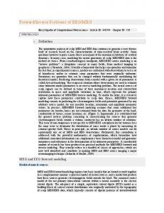
Fig. 1. Examples of the simulated source pdfs (black lines) and their estimation using the LCMV beamformer (blue lines) and the non-Gaussian method (red lines).

matrix Ry, then the conditional density p(s|yt) given by Eq. (15) is also Gaussian with mean value given by Eq. (18) and covariance matrix given by Eq. (19). Furthermore, the marginalised distribution s gs(s) given by Eq. (16) is zero-mean Gaussian with covariance matrix equivalent to Eq. (19). It is notable that the non-Gaussian MD source localisation is also related to the beamformer with general linear constraint (Van Trees, 2004) under the Gaussianity assumption (see Appendix C for further details).

N. This equation implies that constructing the whole measurement pdf gy(y) for any given value of y is unnecessary, and instead, we only need to estimate gy(fs) which is a univariate function. Therefore, the pdf at a location with lead-field matrix f, based on the Eqs. (13) and (20) is given by: XT

  1 K y −h fs h : g s ðsÞ ¼ XTt¼1   ∫ t¼1 h1 K y −h fs ds t

N

ð21Þ

t

N

A kernel based estimation of the measurement pdf We have shown how the source pdf can be estimated from the data pdf. Thus, to implement the method, estimation of the measurement pdf gy(.) is needed from the set of discrete observations yt, t ∈ {1, …,T}. The success of the method depends somehow on the quality of this estimation. Since the dimension of yt is large (on the order of hundreds), we employ kernel based methods, which are fast estimators requiring no optimisation procedure. Kernel based estimation, which is one of the most common methods, assumes that the data pdf may be modelled as the sum of T kernels centred at each observation (Silverman, 1999). Eq. (13) shows that we require gy(fs) to be able to estimate the source pdf, which can be obtained using the kernel density estimator as:   T X 1 y −fs K t g y ð fsÞ ¼ N h t¼1 h

ð20Þ

where K : RN →R is the kernel, h is a scaling factor known as bandwidth, N is the number of sensors, and hN indicates h to the power

Note also that the same kernel based estimation can also be employed for the non-Gaussian method for correlated sources using Eq. (16). To better clarify the algorithm, suppose that at time instant t and at a location with lead-field f, we are interested in estimating the source pdf and consequently the source time-series st. The source pdf is approximated by a set of discrete points within a limited interval (e.g., for s from −10 to 10 with an increment of 0.1), and the value of each point is estimated using Eq. (20). This gives us a scaled version of the source pdf and should be normalised by its integral. The integral is calculated numerically based on the above set of points, resulting in an estimation of the source pdf. This procedure may be repeated for each location and for each time instant. The kernel itself and the bandwidth both need to be chosen; we use the common Gaussian kernel, which is given by (Silverman, 1999):   1 T −1 K ðxÞ ∝ exp − x R ker x 2

where Rker is the covariance of the kernel. The choice of covariance matrix of the kernel is important in determining the spatial resolution. The simplest choice is the identity matrix 1

0.9 Beamforming

0.8

Non−Gaussian method

0.8 0.7

MSE

0.6

MSE

Beamforming

0.9

Non−Gaussian method

0.7

0.5 0.4

0.6 0.5 0.4

0.3

0.3

0.2

0.2

0.1

ð22Þ

0

1

2

3

4

0.1

0

0.5

1

1.5

2

Kurtosis

Kurtosis

a

b

2.5

3

3.5

4

Fig. 2. Comparison between the LCMV beamformer and the non-Gaussian method in the simulated data when (a) one of the sources is non-Gaussian and (b) the additive noise is nonGaussian. The method proposed is insensitive to the non-Gaussianity of the source plus noise.

H.R. Mohseni et al. / NeuroImage 87 (2014) 444–464

1.4

others, as is also the case with the multiple signal classification (MUSIC) algorithm (Mosher et al., 1992).

Beamforming Non−Gaussian method

1.2

MSE

1 0.8 0.6 0.4 0.2 0 0.1

0.2

0.3

0.4

449

0.5

0.6

0.7

0.8

0.9

α Fig. 3. MSE versus correlation between sources for the proposed method and for the classic LCMV beamforming approach in a simulation experiment. The LCMV beamformer is more sensitive to the correlation between sources than the proposed method.

Rker = I, which results in a homogeneous kernel. An alternative efficient choice of covariance matrix of the kernel can be made with the eigenvectors associated with the largest eigenvalues of the measurement covariance matrix. To construct this kernel suppose that Ry = UΣUT is the singular value decomposition of the estimated measurement covariance matrix, and set

Computational complexity Kernel based estimators are almost asymptotically unbiased for a large number of measurement samples (see Appendix D), however, the algorithm is computationally intensive if the number of measurement samples is large. The computational complexity of the proposed algorithm for calculation of the time-series and power at a single voxel is of order O(T2N2Ds) and O(TN2Ds), respectively, where Ds is the number of points that are used to approximate the distribution of one dimensional source. Depending on the number of time samples T and number of points Ds, these orders are generally much bigger than the computational complexity of the LCMV beamformer which is of order O(TN2) for calculation of time-series and O(N2) for calculation of power. For example, estimation of the time-series at each voxel, based on a segment of 30-second MEG data with sampling frequency of 250 Hz, requires approximately 7 s, using a desktop computer with 2.93 GHz CPU. This means that approximately 3 h is required to estimate the timeseries for a set of voxels within the brain with a grid resolution of 12 mm. Compared to the standard beamformer, which needs few seconds to scan the whole brain, the computation time is substantially longer. However, given the fact that MEG source localisation is normally implemented offline and the algorithm may be readily parallelised, this high complexity should not present a barrier to its use. Experimental results

T

Rker ¼ Umax Umax þ σ I where Umax is the matrix containing the eigenvectors associated to the largest eigenvalues, and σ is a regularisation parameter used to stabilise the calculation of the inverse, since UmaxUTmax is rank deficient. This choice of kernel is especially helpful in our study, in which we employed the signal space separation artefact rejection algorithm (Taulu and Simola, 2006). This filtering reduces the rank of the data from number of sensors N to a much smaller number (order of tens). This kernel, which is homogeneous in the space that the data is distributed and is zero elsewhere, can improve the data pdf estimation and therefore results in a better source pdf estimation. In the above equation, Rker is N × N, where N is the number of sensors, and Umax is N × r, where r is the rank of the measurement after applying the signal space separation filter. This choice of kernel can also be useful when some of the eigenvalues of data covariance matrix are considerably smaller than the

Two sets of results are described. The first set uses simulations to investigate and quantify the errors of the methods proposed resulting from non-Gaussian sources and noise. The second set investigates the methods on real MEG data for resting state, auditory and visual stimuli. In each case the methods are compared with the LCMV and null beamformer. Simulation experiments To evaluate the new methods, we ran several simulation experiments. Each used a single layer realistic head model in which the brain was divided into a number of cells. The distance between adjacent cells was 5 mm. The number of samples was 400 and the number of sensors was set to 102 following the number of magnetometer sensors used in our MEG scanner.

3

3.5 Beamforming

Beamforming

Non−Gaussian method

2.5

2.5

MSE

MSE

2 1.5

2

1

1.5

0.5

1

0

Non−Gaussian method

3

0

1

2

3

4

0.5

0

0.5

1

1.5

2

Kurtosis

Kurtosis

a

b

2.5

3

3.5

4

Fig. 4. Comparison between the classic null-beamformer and the proposed non-Gaussian method based on the marginalised distribution for highly-correlated sources when (a) one of the sources is non-Gaussian and (b) the additive noise is non-Gaussian. The method proposed is insensitive to the Gaussianity of the source plus noise.

450

H.R. Mohseni et al. / NeuroImage 87 (2014) 444–464

The data were normalised such that their maximum value was equal to one. In the non-Gaussian method the pdf of each source was estimated over a compact interval between −10 and 10. In all the simulations, the value of the bandwidth in the non-Gaussian method was set to h = 1, and the regularisation factor in the beamformer approach was set to λ = 0.01Tr{Ry} (1% of the trace of the measurement covariance matrix). Note that as long as the covariance matrix is full rank and not nearly rank deficient, the small value of λ has little impact on the results. The first experiment illustrates the estimation of the source pdf for a single non-Gaussian source using the non-Gaussian PD beamformer. The next two examine quantitatively the use of this method on non-

Gaussian noise and correlated sources respectively. In each case the results are compared with the LCMV beamformer. The experiment in the Investigation of null-beamformer and its non-Gaussian extension section compares the performance of the non-Gaussian MD beamformer with the LCMV null-beamformer on the same data. The Reconstruction of simulated sources section extends the investigation of the nonGaussian PD beamformer to image reconstruction for a set of uncorrelated Gaussian sources with non-Gaussian noise. The results from the LCMV beamformer and the SAKETINI method (Zumer et al., 2007) are also provided. Finally, in the Reconstruction of simulated correlated sources section, we show the reconstruction of the time-series using

Fig. 5. An example for reconstruction of six simulated dipoles, (a) original location of dipoles, (b) estimated locations using the LCMV beamformer and (c) estimated locations using the SAKETINI method (Zumer et al., 2007) and (d) estimated locations using the proposed non-Gaussian approach. The non-Gaussian method reconstructed six sources more accurately than the other two methods which assume that the data is Gaussian.

H.R. Mohseni et al. / NeuroImage 87 (2014) 444–464

451

Fig. 6. An example of the reconstruction of six simulated dipoles when the two frontal sources are correlated using (a) the LCMV null beamformer and (b) the non-Gaussian method, while cancelling the left frontal source. The beamformer approach shows spurious activity between the two sources due to the correlation between sources, but the non-Gaussian approach shows more accurate results. There is activity around the left frontal source, using both approaches, because of the additive noise.

the non-Gaussian PD beamformer for non-Gaussian sources, comparing the results with the LCMV beamformer and Bayesian PCA method (Woolrich et al., 2011) as appropriate. Impact of non-Gaussian source In the first simulation experiment, the method was demonstrated through the reconstruction of a single source. Three different pdfs were assigned to the source in turn, the first Gaussian and the others non-Gaussian (described further in the next experiment). It was assumed that in addition there were 15 uncorrelated (Gaussian) sources whose locations were randomly allocated inside the brain volume. The pdfs of the source of interest are shown in Fig. 1. Zeromean Gaussian white noise was also added to the simulated MEG data (after projection of the simulated sources through the leadfields) to set SNR = 8 dB. SNR is defined in the sensor space as the ratio between mean power of the signal to the mean power of the noise across all sensors. The pdf of the first source was estimated using both Gaussian and non-Gaussian assumptions. Fig. 1(a) shows

the result for the Gaussian source where both beamformers give an accurate estimation. Figs. 1(b) and (c) show the results for two nonGaussian sources. It is clear that the non-Gaussian PD beamformer increasingly outperforms the LCMV beamformer as the source pdf deviates more from a Gaussian distribution. In the second simulation experiment, the mean squared error (MSE) resulting from non-Gaussianity of one source was quantified using a Monte Carlo simulation. This source was generated using a mixture model consisting of two zero-mean Gaussian components. The departure from Gaussianity of the source was quantified using the kurtosis k which is defined by k ¼ σμ −3, where μ4 is the fourth moment and σ is the standard deviation. When the kurtosis is zero, the data is Gaussian, and as it becomes larger, the pdf departs further from a Gaussian profile. Only when the variances of the two pdfs in the mixture model are identical, is the mixture also Gaussian. Fig. 2(a) presents the result of the MSE which is defined as the mean squared error between the original and constructed pdf for different kurtosis. The average SNR is −5 dB and the results were obtained using 1000 Monte Carlo simulations. It 4 4

2 Original Non−Guassian method Beamforming Bayesian PCA

1.5

Amplitude

1 0.5 0 −0.5 −1 −1.5 −2 −0.2

−0.1

0

0.1

0.2

0.3

0.4

0.5

0.6

Time [sec] Fig. 7. Estimation of simulated time-series using the proposed non-Gaussian method (red), the classic LCMV beamformer (blue) and Bayesian PCA (green). The original waveform has been shown by a solid black line.

452

H.R. Mohseni et al. / NeuroImage 87 (2014) 444–464

120

sources, the MSE from the novel non-Gaussian method does not increase very significantly.

100

Investigation of null-beamformer and its non-Gaussian extension Next, we investigated the performances of the null-beamformer and the non-Gaussian MD beamformer designed to cope with correlated sources using the same simulation configuration. The results are presented in Fig. 4. In each case, we assumed that the null location is known. Fig. 4(a) shows the results when one source is non-Gaussian and Fig. 4(b) shows the results when the additive noise is nonGaussian. Both methods are capable of cancelling out the correlated source, but the non-Gaussian MD beamformer is better at dealing with the non-Gaussianity of the source and additive noise.

Kurtosis

80

60

40

20

0

50

100

150

200

Channel Fig. 8. Kurtosis versus channels in resting state experiments recorded from 10 subjects. Kurtosis can be very large in some cases indicating the high non-Gaussianity of the measured MEG.

is clear that as the kurtosis increases, the error in the LCMV beamformer increases rapidly. In contrast, the new non-Gaussian PD beamformer exhibits a flat error which means it is not sensitive to the shape of the pdf. Impact of additive non-Gaussian noise So far the effect of non-Gaussian sources has been considered where the noise was Gaussian. This simulation experiment was devoted to investigating additive non-Gaussian noise. In this case, all sources were Gaussian and the noise was generated as per the previous example by using a Gaussian mixture model with two zero-mean Gaussian components. The covariance matrix of one of the Gaussian components was the identity matrix I and the covariance of the second Gaussian component was aI, where σ was varied to gain different values of kurtosis. As demonstrated by Fig. 2(b), the non-Gaussian method is insensitive to the shape of the noise pdf whereas the MSE in the LCMV beamformer increases with increasing kurtosis. Impact of correlation between sources This experiment assesses the effect of correlated sources on the LCMV beamformer and the non-Gaussian PD beamformer. Here, the sources and the additive noise were all assumed to be Gaussian. Two correlated sources s1 and s2 were generated using standard Gaussian distribution: s1 ∼N ð0; 1Þ; s2 ∼ð1−α ÞN ð0; 1Þ þ αs1, where α is a measure of correlation between sources; α = 0 means the sources are uncorrelated and α = 1 means they are completely correlated. The locations of the two sources were randomly and uniformly set within the brain in the Monte Carlo simulation to estimate the average impact of the method over all locations. Fig. 3 shows that even for Gaussian sources the non-Gaussian method shows a better reconstruction of the desired source pdf than the LCMV beamformer as the correlation between sources increases. Even with moderate correlation between

Reconstruction of simulated sources In the next simulation experiment, we simulated six uncorrelated Gaussian sources with non-Gaussian noise to compare the source localisation accuracy of the LCMV beamformer and the non-Gaussian PD beamformer. The noise was created as in the other experiments with the kurtosis equal to 3. The location of the sources is shown in Fig. 5(a) and marked by green dots. The sources in this example were also reconstructed using the SAKETINI method (Zumer et al., 2007), which is a graphical model and assumes that a segment of the noise and the number of sources are known. The noise segment was generated with the same distribution as that of the additive noise used to simulate the measurements. The number of sources was set to 6 and the algorithm was implemented using the NUTMEG toolbox with the recommended settings (Dalal et al., 2004). The results using the LCMV beamformer, SAKETINI and the nonGaussian PD beamformer are shown in Figs. 5(c–d). The source activities estimated using the three methods have been normalised between 0 and 1. It is clear that the new method gives more accurate reconstruction, particularly, with higher spatial precision for frontal and temporal sources. Reconstruction of simulated correlated sources We also investigated the impact of correlated sources on the source reconstruction. We used the same simulation settings as the previous example, but the two frontal sources are chosen to be completely correlated, i.e., the same time-series. If we reconstruct these correlated sources without the nulling technique, a spurious source between the two correlated sources is estimated. We therefore assume that the location of one of the correlated sources (left frontal source) is known, and then place a null at its location. The results using LCMV and the nonGaussian method are shown in Fig. 6, in which due to non-Gaussian noise, the LCMV beamformer shows inferior localisation compared to the non-Gaussian method. Estimation of simulated time-series In the last simulation experiment, we examined the accuracy of estimation of the underlying time-series. The location of the desired source is the right frontal source as shown in Fig. 5(a). The shape of the original time-series is shown in Fig. 7 with a solid black line. It consists of two cycles of a sinusoidal wave within a period of no activity to represent an event-related field potential. We also compare the proposed method with a recent method based on the Bayesian PCA for estimation of the

Fig. 9. Histograms of the first seven channels for data in a 100–150 ms interval after stimulus onset in a visual paradigm. The histogram should be in the form of Gaussian function (bell shape) to effectively employ the classical LCMV beamformer.

H.R. Mohseni et al. / NeuroImage 87 (2014) 444–464

453

Fig. 10. Reconstruction of neural activity in the visual paradigm using beamforming with (a) λ = 0.01%, (b) λ = 0.01% and (c) λ = 1% of trace of data covariance matrix, and using nonGaussian method with (d) h = 1, (e) h = 5 and (f) h = 10.

454

H.R. Mohseni et al. / NeuroImage 87 (2014) 444–464

Fig. 11. Reconstruction of neural activity in the auditory paradigm using LCMV beamformer with (a) λ = 0.01%, (b) λ = 0.1% and (c) λ = 1% of trace of data covariance matrix, and using the proposed non-Gaussian method with (d) h = 1, (e) h = 5 and (f) h = 10.

H.R. Mohseni et al. / NeuroImage 87 (2014) 444–464

covariance matrix. This method particularly is useful when there are few sources and therefore the covariance matrix can be represented by a few eigenvectors (for further details please refer to (Woolrich et al., 2011)). The estimated time-series using the non-Gaussian PD beamformer, the LCMV beamformer and Bayesian PCA were plotted using red, blue and green lines, respectively, in Fig. 7. These results imply that the non-Gaussian methods outperform the LCMV when the observations are non-Gaussian. The proposed method also outperforms the Bayesian PCA approach when the signal is corrupted with an additive nonGaussian noise. This is because the Bayesian PCA only uses the second order statistics and therefore still assumes that the observations are Gaussian. Experiments using MEG data Data acquisition Ethical approval of the research methods was obtained on 18 July 2008 from Oxfordshire Research Ethics Committee (reference: 08/ H0604/58). The MEG data were recorded from three cohorts of 12 participants, all of whom were given informed written consent before taking part in the studies. We compared the performance of the non-Gaussian method with the LCMV beamformers on data from three separate MEG experiments. The resting state experiment used ten right-handed participants (4 males, age 22–45 years) under the condition of eyes open with fixation. The visual experiment used a 27-year-old right-handed female with normal vision or vision corrected to normal. The auditory experiment used a 24-year-old right-handed participant with normal hearing. All MEG recordings were performed using a 306 channel Elekta Neuromag system with 102 magnetometers and 102 pairs of planar gradiometers. Data were recorded at a sampling rate of 1000 Hz with a 0.1 Hz high pass filter. Prior to acquisition, a three-dimensional digitizer (Polhemus Fastrack) was used to localise the participants' head shape relative to the position of the head-coils, with respect to three anatomical landmarks which could be registered on the MRI scan (the nasion, and the left and right preauricular points). A structural MRI was also acquired for each participant. A single layer realistic head model was used in the source analysis of both the visual and auditory experiments. Head movements were kept to a minimum, and head positions were localised immediately before the start of the experiment. Signal space separation or MaxFilter, which is a commercial pre-processing software package recommended by the Elekta company, was applied to the continuous data (Taulu and Simola, 2006). The continuous measurements were then linearly filtered in a bandpass range of 1–40 Hz. The data were segmented and a baseline correction applied (using a 200 ms segment of data before the stimuli). Finally, the trials were visually inspected and those with large variations were removed. Investigation of Gaussianity of MEG data In the first experiment, we examined the Gaussianity of real MEG data recorded from ten normal participants in the resting state through estimating the kurtosis. The kurtosis of the gradiometer signals is plotted in Fig. 8 (sorted in order of descending kurtosis for each subject for clarity). It is clear that even for resting state data, the kurtosis in some cases can become very large meaning that the data pdf is highly non-Gaussian. As a further test, the Jarque–Bera goodness-of-fit test (Jarque and Bera, 1987) was applied to both skewness and kurtosis. The test implied that only two channels in one subject and one channel in another subject were Gaussian distributed with p b 0.05. We conclude therefore that an assumption of Gaussianity is not valid for real MEG data. In the following experiments, we compared the performance of the methods for source reconstruction and investigated the sensitivity of

455

the results with regard to two key parameters λ and the kernel bandwidth h. Visual paradigm The second MEG experiment used a visual paradigm where a series of human and animal faces were presented to the participant. Each image was presented for 300 ms and the time interval between images was 1500 ms. We were interested in localising the first significant peak of averaged epoched data which occurs around 100–150 ms after the onset of visual stimuli. The origin of this peak is known to be located in bilateral regions of the primary visual cortex. Fig. 9 shows the histogram of this peak for the first five channels; none matches a Gaussian distribution. Based on the results from the simulation experiments, we therefore would expect the non-Gaussian method to outperform the standard beamforming approaches. This was confirmed in Fig. 10. Figs. 10(a)–(c) show the output power of the beamformer (trace of the estimated covariance matrix as in Eq. (4)) normalised by the norm of the associated lead-fields; i.e., normalised by the power of projected white Gaussian noise (see (Van Veen et al., 1997)). Figs. 10(d)–(f) show the estimated power using the non-Gaussian PD beamformer, which was also normalised by the norm of the associated lead-fields. In both methods, the same anatomical plane is displayed and it includes the results for different values of λ and h. For the LCMV beamformer, we see from the figure that if a small value for λ is chosen, the peak of the spectrum is in a frontal part of the visual cortex and if a large value is chosen, the peak of reconstructed source is in the cerebellum and not in the visual cortex. In contrast the non-Gaussian method reconstructs activity in both right and left primary visual cortex for moderate and small values of h. It also has better spatial resolution. Auditory paradigm The third MEG experiment was particularly useful to compare the performance of both sets of beamformers: the LCMV beamformer with the non-Gaussian PD beamformer and the null-beamformer with the non-Gaussian MD beamfomer. It used a mismatch negativity auditory paradigm, where participants were presented with trains of 7 different tones repeated randomly. The frequency of the tones increased from 500 to 800 Hz in steps of 50 Hz. The number of times that the same tone was presented in the sequence varied pseudo-randomly between one and eleven. The probability that the same tone was presented once or twice was 2.5%, three and four times was 3.75% and five to eleven times was 12.5%. Stimuli were presented biaurally via headphones for 15 min. The duration of each tone was 70 ms, with 5 ms rise and fall times, and the inter-stimulus interval was 500 ms. Here, the first tone of each train is considered as deviant and the rest as the standard tone. About 250 deviant trials were presented. We were only interested in localising a significant peak known as N100 which occurs 100 ms after the stimulus onset. The source of this peak is known to be in bilateral regions of the primary auditory cortex. Traditional beamforming methods have been shown to have difficulty in reconstructing these bilateral sources correctly. The results of the source reconstruction are presented in Fig. 11 using the non-Gaussian PD and LCMV beamformers. In all the figures, the small green volume is the mask representing the primary auditory cortex presented using the Juelich Histological Atlas (Morosan et al., 2001). Figs. 11(a)–(c) show the results using the LCMV beamformer (blue regions) with λ equal to 0.01%, 0.1% and 1% of the trace. It is clear that, depending on the value of λ, the LCMV beamformer has only reconstructed a source primarily in the left or right auditory cortex, leaving out the source in the other cortex. In addition, it has placed an extraneous source in the middle of the brain (close to the precuneus and posterior cingulate cortex), and one deep in the brain. These extraneous sources are likely to arise from correlations between genuine sources. Figs. 11(d)–(f) show the results from the non-Gaussian method for h = 1, 5 and 10, respectively. It shows better reconstruction

456

H.R. Mohseni et al. / NeuroImage 87 (2014) 444–464

Fig. 12. Reconstruction of neural activity in the auditory paradigm when the right-hand side source is cancelled out using the classic null-beamformer with (a) λ = 0.01%, (b) λ = 0.1% and (c) λ = 1% of trace of data covariance matrix, and when the right-hand side source is cancelled out using the proposed marginalised based non-Gaussian method with (d) h = 1, (e) h = 5 and (f) h = 10.

H.R. Mohseni et al. / NeuroImage 87 (2014) 444–464

of both left and right sources in the primary auditory cortex (especially for h = 5). It does not show any source deep in the brain, but for higher values of h it does present a potentially incorrect source in the middle of the brain due to the high correlation between sources. These observations also show that the sensitivity of the new method to the choice of bandwidth h was no higher than the sensitivity of the LCMV beamformer to regularisation factor λ. Since the two sources are partially correlated, the classic nullbeamformer and the non-Gaussian MD method were employed to cancel out one of the correlated sources. Figs. 12(a)–(c) show the results from the classic null-beamformer when a null has been placed at the right auditory cortex with three different values of λ. The nullbeamformer shows activity near the left auditory cortex and has reduced the large source of activity in the middle of the brain for small values for λ but shows significant areas of extraneous activity as λ is increased. Figs. 12(d)–(f) show the equivalent results using the nonGaussian approach. It is clear that the source in the left auditory cortex had been located and other extraneous sources reduced. The nonGaussian method shows less sensitivity to its parameter h than the null-beamformer does to its parameter λ. Fig. 13 presents similar results to the previous figure, but here the null has been placed in the left auditory cortex. The results of the null-beamformer with different values of λ are shown in Figs. 13(a)–(c). While the large sources of activity in the middle and deep structure of the brain have largely been suppressed, the source in the right auditory cortex is not at the correct location. In contrast, Figs. 13(d)–(f) demonstrate the superior results from the non-Gaussian method, which localises the source of activity very close to the expected location. The extraneous sources have also been completely removed. Resting state One of the resting state networks which has been well identified in both fMRI and MEG data is the sensorimotor network (see (Brookes et al., 2011) for more details). We use this network as a ground truth to further investigate the performance of the proposed method. A 30second segment of raw MEG data were filtered in the beta band (13–30 Hz) and the time-series at each voxel were estimated. The correlation between the Hilbert envelope of the time course of the seed source, located at the right sensorimotor cortex, with the envelopes for the time courses at each voxel was then estimated. The results for the LCMV beamformer and the proposed non-Gaussian method are presented in Fig. 14. The activity at the left sensorimotor cortex, as reconstructed by the LCMV beamformer, does not show any correlation with the right sensorimotor cortex, while the activity, reconstructed by the non-Gaussian method, shows a correlation of about 0.4. This example also demonstrates the better performance of the proposed method over the standard LCMV beamformer. Summary and discussion In this paper, we introduced a probabilistic formulation for MEG source localisation which allows non-Gaussian measurements to be modelled. An extension of the method to handle correlated sources through the marginalisation of the estimated joint pdf was also presented. The implementation of the new method showed that it outperforms existing LCMV beamforming methods in terms of spatial and temporal source estimations in data from simulations and real MEG experiments. In particular, in the simulation experiments, we showed that the non-Gaussian methods are superior to the LCMV beamformers in coping with non-Gaussian pdfs for source and additive noise, and for correlated sources. In addition, the mean square error in estimating non-Gaussian time-series was also less. The improved results for simulation experiments were repeated when the method was applied to real MEG data. The non-Gaussian beamformer was again superior in

457

localising visual and auditory paradigms, where the latter is known to contain sources with high correlation. Here, we used the kernel density estimator to estimate the data and consequently the source distribution. Based on Algorithm 1, it is clear that any other multivariate density estimator such as mixture of Gaussian functions or multivariate Edgeworth series (Davis, 1976) could also be employed. Analysis of the impact of these approaches on the source localisation is beyond the scope of this paper, and we plan to evaluate their performances in the near future. One criticism of this approach is that estimation of high dimensional density normally is not feasible because of the lack of enough observations. However, we present the following arguments to show that kernel density estimators are suitable in MEG source localisation: • Importantly, although in theory we assume that the multivariate data distribution gy(y) is known, in practice we do not estimate this multivariate distribution and only estimate a univariate function gy(mathbffs) — see A kernel based estimation of the measurement pdf section and specifically Eq. (20). The reason for this simplification is that this method assumes, as the traditional beamformer, that all sources are independent and thus it is not required to estimate the inter-dependency of sources. However, it is notable that in the proposed approach for correlated sources, when we need to estimate the multivariate joint distribution, it is required that we estimate the inter-dependency of sources. In this case, the number of correlated sources to be estimated should not be overly high, because it may not be feasible to estimate a high dimensional distribution. • Although we suggest the use of kernel density estimators in the application of the MEG source analysis, the problem of high-dimensionality in multivariate density estimators is not limited to this method and has been discussed in other applications. For instance, for the purposes of statistical discrimination, Scott (1992) and Scott and Sain (2004) argued that kernel methods are powerful tools even over dozens of dimensions. This is because if the bandwidth is very small, the kernel estimate is essentially a nearest-neighbour classification, and if the band-width is very large, the result is the Fisher's linear discriminant analysis. Thus, at the extremes, kernel density analysis mimics two successful algorithms and an appropriately chosen value for the bandwidth should outperform both algorithms. Here, we also observed that if we select the covariance of the kernel equal to the covariance of the observed data then the kernel density estimator and the LCMV beamformer show similar results. • Other factors including SNR and correlation between sources, generally have more impact on a MEG source reconstruction algorithm than the number of observations. For example, only one sample is enough to exactly estimate the location of one source in a high SNR data set, while it is impossible to estimate the covariance matrix based on only one sample. On the other hand, if we have a very low SNR, the exact estimation of the covariance matrix or data distribution, obtained from a large number of observations, does not necessarily help to localise the source activity. We may conclude from the above points that the ultimate aim of beamforming is source reconstruction and not estimation of the covariance matrix or data distribution. This has again been discussed in the statistical discrimination applications by Friedman (1997), who argued that the optimal bandwidth for kernel discrimination is normally much larger than for optimal density estimation. Therefore, the bandwidth or form of the kernel (or regularisation factor in the beamformer) should be chosen such that the best source localisation and not the best density (or covariance matrix) estimation is achieved. Comparison to the other related methods To date, several methods have been proposed to tackle or exploit the non-Gaussianity of the MEG data set. Specifically, Nagarajan et al. (2005, 2006) proposed a generative model for ERF data that uses pre-stimulus

458

H.R. Mohseni et al. / NeuroImage 87 (2014) 444–464

Fig. 13. Reconstruction of neural activity in the auditory paradigm when the left-hand side source is cancelled out using the classic null-beamformer with (a) λ = 0.01%, (b) λ = 0.1% and (c) λ = 1% of trace of data covariance matrix, and using the proposed marginalised based non-Gaussian method with (d) h = 1, (e) h = 5 and (f) h = 10.

H.R. Mohseni et al. / NeuroImage 87 (2014) 444–464

data segments to learn noise and interference components, thereby allowing for the rejection of noise and interference from post-stimulus segments. This method, which is based on factor analysis, models the source activity by a mixture of Gaussian functions to incorporate the non-Gaussianity of the evoked brain sources. Although this method assumes that the sources of interest are non-Gaussian, other distributions including the noise and artefacts are assumed to be Gaussian. Conversely in the approach proposed here we assumed that the measurements are non-Gaussian, which includes both the source and noise components. Moreover, in Nagarajan et al. (2005, 2006), it is assumed that the noise and artefact in the pre-stimulus and post-stimulus segments are statistically the same, whereas in the proposed approach we do not exploit information obtained from pre-stimulus segments. It is also clear that the method proposed in Nagarajan et al. (2005, 2006) can be used for the purpose of noise and artefact rejection before employing any source reconstruction method including our proposed approach. The method described in Nagarajan et al. (2005, 2006) has been extended by Zumer et al. (2007, 2008) by incorporating the lead-field of the source of interest and also by including temporal basis functions for modelling the MEG signals. In contrast to the method in Nagarajan et al. (2005, 2006) and the method presented here, Zumer et al. (2007, 2008) assume that all distributions are Gaussian. This is partly to require fewer parameters to be estimated, which in turn leads to a robust estimation with less dependency on the initialisation step. They have also related their approach to the traditional beamformer and demonstrated that the beamformer is algebraically equivalent to the maximum likelihood approach based on a uniformly distributed prior (Zumer et al., 2007). Here we have verified this finding and used this result to extend the method to non-Gaussian distributions (see Eq. (8)). Moreover, the proposed non-Gaussian method maintains one of the potential benefits of the LCMV beamformer, in that it is less dependent on a generative model describing the MEG data as a function of dipole sources and their corresponding lead fields. ICA is another method that uses the non-Gaussianity of MEG data and has been extensively employed for artefact rejection or dimensionality reduction. As in the method presented here, ICA assumes that the data is stationary but not Gaussian. It is also clear that, in contrast to

459

our method, ICA does not use spatial information, specifically the leadfield matrices, and also uses measures of the non-Gaussianity, such as kurtosis, rather than the data distribution. Markov Chain Monte Carlo (MCMC) is another method that allows for non-Gaussianity (Jun et al., 2005). MCMC is an alternative to variational Bayes and its advantages over variational methods have been shown by Nummenmaa et al. (2007), when the posterior distribution is not uni-modal. As with our proposed method, MCMC uses sample points to estimate the distribution, which leads to a computationally intensive method. The main difference between MCMC and our approach is that MCMC assumes that the posterior distribution of the parameters of the model is non-Gaussian rather than the distribution of the measurements. This prevents the algorithm from being trapped in local minima, yet does not address the non-Gaussianity of the MEG signals. In the case of measurement data from a large number of sensors, it has been argued that dimensionality reduction is often necessary (Zumer et al., 2007). The dimensionality reduction used here was performed using the signal space separation algorithm by projecting the data into the space that represents the internal volume of the sensors (see (Taulu and Simola, 2006) for more details). Other methods for dimensionality reduction as well as noise and artefact rejection such as PCA and ICA, can also be employed to improve the current approach. PCA may fail in low SNR data and give erroneous results, and other approaches like factor analysis (Nagarajan et al., 2006) and Bayesian PCA (Woolrich et al., 2011) seem more appropriate, where a robust estimate of the noise covariance is made. Finally, we assumed that the prior of the source is uniformly distributed (no prior information on s) which leads to a simple form of posterior distribution. This is in line with several other methods in the estimation theory literature including pseudo-inverse, maximum likelihood, LCMV beamformer, particle filters, and minimum norm source estimation. Nevertheless, the proposed method can be extended by using a prior obtained from anatomical information. One way, as described in Limpiti et al. (2006), is to use a cortical patch as a source model for representing spatially distributed neural activity based on a set of basis functions. Similarly, we may also incorporate prior assumptions about the source configuration obtained

Fig. 14. Correlation between the Hilbert envelope of the right sensorimotor cortex and all other voxels for MEG data filtered within the beta band, (a) results from the LCMV beamformer and (b) results from the non-Gaussian method. The non-Gaussian method shows a correlation with the left sensorimotor cortex, while the LCMV beamformer does not show any correlation.

460

H.R. Mohseni et al. / NeuroImage 87 (2014) 444–464

from structural MRI. Such models have already been developed in a Bayesian framework in the context of distributed source localisation (Mattout et al., 2006). The method introduced in this paper has shown clear advantages over the LCMV beamformer, which uses second order statistics to represent non-Gaussian data. Through a stochastic formulation and kernel density estimation, the method offers a general representation of the source pdf. Although the implementation presented uses a non-informative prior on the source pdf, the method allows a prior to be incorporated. The method currently implemented is based on scalar sources; however the general formulation is readily applicable to vector source localisation, although the complexity would be greater. We believe that the methods introduced here provide a useful contribution to MEG imaging by relaxing a strong assumption in the LCMV and nullbeamformer. Acknowledgments

where α = ∫ gn(Fs)ds, and range of a matrix F is uj∃s∗ ∈ Rq such that u ¼ Fs∗ Proof. Suppose there is a s⁎ such that y = Fs⁎, so           αg s s ¼ g s s ∫g n ðFsÞds ¼ gs s ∫g n F s −s ds:

          g ðyÞ−αg s  ¼ ∫g ðsÞg ðy−FsÞds−g s ∫g F s −s ds y s s n s n     ≤∫gs ðsÞ−g s s gn ðy−FsÞds:

There is no conflict of interest. Appendix In this section, the theoretical analysis of the proposed method is presented. Appendix A shows that the source pdf can be exactly estimated if the noise power is very small and sources are independent. These results assure that a reliable approximation of the source pdf is obtained in the case of a high SNR data set. Appendix B shows that the proposed method is equivalent to the null-beamformer in the case of Gaussian measurements. Appendix C shows the relation of the proposed method to the well-known beamformer with general linear constraint, which is a generalisation of the null-beamformer. Appendix D presents the convergence analysis and convergence rate of the algorithm based on the multivariate kernel density estimation.

ð25Þ

Now Let δ N 0, and split the region of integration into two regions |s — s⁎| ≤ δ and |s − s⁎| N δ such that ∫ ¼ ∫js−s∗j ≤ δ þ ∫js−hbf s∗ j N δ ¼ I1 ðyÞ þ I 2 ðyÞ. Then we have: Z

js−s j ≤ δ

js−sj ≤ δ

g n ðy−FsÞds

ð26Þ

by continuity of gs(s), the above value is small for δ that is sufficiently small. On the other hand, for δ fixed we have Z jI 2 ðyÞj≤



js−s j N δ

Z

≤2M

Conflict of interest

ð24Þ

Therefore using Eq. (1):

     I ðyÞ ≤ max g ðsÞ−g s  1 s s 

This work is funded by The Wellcome Trust and Engineering and Physical Sciences Research Council UK (EPSRC) under grant number WT 088877/Z/09/Z. M. L. Kringelbach is funded by the TrygFonden Charitable Foundation and T. Z. Aziz is funded by the Medical Research Council, the Norman Collisson Foundation and the Charles Wolfson Charitable Trust.

Rð FÞ ¼

    g ðsÞj þ jg s  g ðy−FsÞds s s n ð27Þ

js−sj N δ

g n ðy−FsÞds

where M is the maximum of gs(s). Noting that because |s − s⁎| N δ there is a fixed ϵ such that |y − Fs| = |F(s⁎ − s)| N ϵδ. This means I2(y) tends to zero by explicit assumption about the noise (∫|n| Nδ gn(n)dn → 0). Now suppose there is no s⁎ such that y = Fs⁎, but that there is a δ N 0 such that |(s⁎ − s)| N δ and there is ϵ N 0 such that |F(s⁎ − s)| N ϵδ, for all s ∈ ℝq. Therefore Z g y ðyÞ≤M

js−sj N δ

g n ðy−FsÞds

ð28Þ

where M again is the maximum of gs(s). Using the same argument as in Eq. (27), gy(y) tends to zero. ■ Using the above Lemma it is now shown that gy(fksk) is the exact estimation of g sk ðsk Þ. If we set s* = [0…0…sk…0…0]T, then y = Fs⁎ gives y = fksk. Using Lemma 1:

A. Impact of the noise Below, we show that Eq. (13) gives the exact source pdf, if the noise power is considerably lower than the signal and interference power. We can say that the noise power tends to zero, if ∫|n| Nδ gn (n)dn → 0 for all δ N 0, where |.| denotes the Frobenius norm. An example of such noise is the multivariate Gaussian whose norm of the covariance matrix tends to zero. Theorem 1. In addition to the assumptions stated in Problem formulation section, suppose that the noise power tends to zero, and the lead-field vectors fi, i = 1,… q, are mutually independent. Then g sk Þ ðsk Þ can be exactly estimated by ∫gg ððff ssÞds , where the normalising constant y

k

y

k

is also given by ∫g y ð f k sÞds ¼ g sk= ð0Þ∫g n ðFsÞds. Proof

ð29Þ

where Z ¼ αg sk= ð0Þ ¼ g sk= ð0Þ∫g n ðFsÞds . Eq. (29) gives g sk ðsk Þ ¼ g y ð f k sk Þ=Z , where Z also is a normalising constant Z = ∫ gy(fk sk) dsk. ■ Given this result we can now investigate the estimated source pdfs in a noisy environment. First, note that the relationship between the measurement pdf and the source pdf in addition to the noise pdf based on Eq. (1) is given by the following equation (the pdf of the sum of two random variables (Grimmett and Stirzaker, 2001)): Z g y ðyÞ ¼ g s ðsÞg n ðy−FsÞds: ð30Þ Rq

  From Eqs. (13) and (30) the pdf of kth source g sk s∗k is given by:

Lemma 1. Based on the assumption in Theorem 1 and pseudo-convolution, we have     αg s s y ∈ Rð FÞ whereby y ¼ Fs g y ðyÞ→ 0 y ∉ Rð FÞ

  g y ð f k sk Þ→αg s s ¼ αg sk ðsk Þg sk= ð0Þ ¼ Zg sk ðsk Þ

ð23Þ

       g sk sk ∝g y f k sk ¼ ∫g s ðsÞg n f k sk −Fs ds ð31Þ

  ¼ ∫∫g sk ðsÞg s= s= gn f k sk −thbf f k sk − F= s= dsds=

H.R. Mohseni et al. / NeuroImage 87 (2014) 444–464

where we assumed that sk is independent from the other sources. By changing the variable sk⁎ − sk = u, we have    

  g y fsk ¼ ∫∫g sk sk −u g s= s= g n fu−F= s= ds= du        ¼ ∫g sk sk −u gy= ð fuÞdu ¼ g sk sk  g y= fsk

Using the Gaussianity of the data, p(s | yt) is found as h
T
i −1 pðsjyt Þ∝∫ exp − fs þ F= s= −yt Ry fs þ F= s= −yt ds= T T

ð32Þ

tional to g sk ðs∗k Þ∗g y= ð fsk Þ. This means that the estimated source pdf is the original pdf that is convolved with an unknown function which is based on the pseudo-convolution of the noise and interference pdfs. This means that in contrast to the noise-free environment, interference can also distort the estimated pdf. It is clear that, if the noise pdf is known for example from prestimulus trials, one can employ the deconvolution method to remove the noise and then estimate g sk ðsk Þ from a noise-free data set.

T

T

−1



Ps ¼ c

F

" ¼ ½1 0  ¼

T

T

−1

T

−1

f Ry f F= Ry f

f Ry

−1

−1

T T

−1

# ! h i −1 T −1 f ¼c f F= c T Ry F= # −1 T −1 f R y F= 1 T −1 0 F= Ry F=

T

T

−1

T

T

−1

T

−1

ð36Þ


−1 T −1 T s= − F= Ry F= F= Ry ð fs−yt Þ ds= 

The last integral is an integration over a Gaussian distribution with random variable s/ and therefore it will be a constant. We continue by eliminating the integral and combining the two exponentials: T

Here, it is shown that if the measurement is Gaussian, p(s | yt) given by Eq. (15) is Gaussian with variance equal to Eq. (19) and mean equal to Eq. (18). Similarly, it can be shown that gs(s) given by Eq. (16) is a zero-mean Gaussian with variance equal to Eq. (19). Using block matrix inversion, the output power of the nullbeamformer, Eq. (19), can be expressed as: 

T




−1 T −1 T −1 T −1 exp ð fs−yt Þ Ry F= F= R y F= F= Ry ð fs−yt Þ

pðsjyt Þ ∝ exp½−s

−1 −1 Ry F c

−1

 T

−1  T −1 T T ∫exp − s= − F= R y F= F= R y ð fs−yt Þ F= R y F=

B. Relation to the null-beamformer

T

T T

−s= F= R y fs−s= F= R y F= s= þ s= F= Ry yt þ f yt R y F= s= ds= h i T T −1 T T −1 T −1 ∝ exp −s f Ry fs þ s f R y yt þ yt Ry fs 

erator. Therefore, Eq. (32) states that the estimation of g sk ðs∗k Þ is propor-




−1

∝∫ exp½−s f Ry fs þ s f R y yt þ yt Ry fs−s f Ry F= s=



 where g y= ð fuÞ ¼ ∫g s= s= gn fu−F= s= ds= and * is the convolution op-

T

461

T



þs




−1 T −1 T −1 T −1 T −1 f Ry f−f R y F= F= R y F= F= R fy f s


−1 T −1 T −1 T −1 T −1 f R y yt þ f R y F= F= Ry F= F= Ry yt

 
−1 T −1 T −1 T −1 T −1 þ yt R y f þ yt Ry F= F= R y F= F= R y f s  


−1 T T −1 T −1 T −1 T −1 ∝exp −ðs−aÞ f R y f−f Ry f F= R y F= F= Ry f ðs−aÞ

"

ð37Þ

T

ð33Þ

−1

−1
T −1 T −1 T −1 f− f Ry F= F= R y F= F= Ry f

where a = (fT Ry− 1 f − fT Ry− 1 (F/T Ry− 1 F/)− 1 F/T Ry− 1 Ry− 1 f)− 1 (fTRy−1yt +fTRy−1 F/(F/TRy−1 F/)−1 F/Ry−1yt). The above equation shows that p(s | yt) is a Gaussian distribution and its variance is equal to Eq. (33). The best estimation of the time-series is its mean which is equal to Eq. (34). C. Relation to the beamformer with general linear constraint

which is the Schur complement. The time-series, Eq. (18), using block matrix inversion is also expanded as: " ^st ¼ ½1 0  ¼

f

T

T

−1

T

−1

f Ry f F= Ry f

T

−1

T

−1

f R y F= F= Ry F=

−1 T −1 Ry f− f R f




#−T "

# T −1 f yt T R F=

−1 T −1 T −1 F= Ry F= F= Ry f

T



−1 f

T

−1 Ry yt

ð34Þ

−1
−1 T −1 T −1 T −1 T −1 f R y f−f Ry f F= Ry F= F= Ry f




−1 T −1 T −1 T −1 T −1 f Ry yt þ f R y F= F= R y F= F= R y yt

where −T denotes transpose and inverse operation. Now we derive the null-beamformer (above expanded equations) using the method proposed. Eq. (15) is rewritten as

 pðsjyt Þ ¼ ∫p s; s= jyt ds= ∝∫p fs þ F= s= jyt ds= :

T

T

argmax w R y w; subject to : w F ¼ c

 −1
−1 T −1 T −1 T −1 T −1 þ f R y f−f R y f F= Ry F= F= Ry f
−1 T −1 T −1 T −1 f Ry F= F= Ry F= F= Ry yt ¼

A beamformer with general linear constraint is given by the following formulation (Haykin, 2002):

ð35Þ

ð38Þ

where F = [f1…fq] and c is a constraint vector. The solution of this problem is the same as those given by Eqs. (18), (19), except that, here, c is an arbitrary vector. Our aim is to present an estimation method for gs(s) that is equivalent to the beamformer with general linear constraint, when the measurement is Gaussian. The method based on the marginal distribution given in the NonGaussian marginal distribution for correlated sources section, marginalises out all the parameters except the desired parameter. In other words, it integrates gs(s) over the subspace that is perpendicular to c = [1 0]T. Therefore, we can employ the same procedure to first estimate gs(s) ∝ gy(Fs), and then the desired pdf gs(s) for an arbitrary c is obtained by integration of gs(s) over the subspace that is perpendicular to c, or equivalently: Z g s ðsÞ ¼

Ωc

g y ðFsÞds=

ð39Þ

where Ωc = {s | cTs − cTcs = 0}, and ∫Ω g ds= is the integral of g over c

subspace Ωc with appropriate variable of integration ds/.

462

H.R. Mohseni et al. / NeuroImage 87 (2014) 444–464

The general solution of the method proposed (Eq. (39)) has the same solution to the beamformer with general linear constraint, when the measurement is Gaussian. This can simply be shown by rotating the coordinate such that the vector c lies on the first axis. In this case, the rotated c is equal to [1 0]T and, thus, Eq. (16) can be used for this rotated coordinate. By rotating back to the original coordinate, Eq. (39) is obtained.

Proof. See Proposition 31.8 in Port (1994). ■   U 1 ðyÞ ¼ h1 K fs−y (nominator of Eq. (21)) and U 2 ðyÞ ¼ ∫h1 K
Suppose  h fs−y ds (denominator of Eq. (21)), then: h

D. Convergence analysis

To calculate the above integral, we rotate the coordinate such that the line along the direction of f lays on the of the first coordinate axis. This can be done simply by a rotation matrix Θ such that Θf = |f|[1 0…0]T, where |f| is the norm of f. Suppose that the rotated pdf and the rotated kernel are gyr(v) = gy(Θy) and Kr(v) = K(Θy), respectively, where v = [v1,…, vn]T is the new coordinate. Thus, Eq. (51) is rewritten as:

The convergence, bias and variance of the kernel based pdf estimation stated in Eq. (21) is given by the following theorem. Theorem 2. Suppose the kernel K satisfies the following conditions: Z

Z K ðuÞdu ¼ 1;

j

T

u uK ðuÞdujb∞; K ðuÞ ¼ K ð−uÞ

N

Z EfU 2 g ¼ E

ð40Þ

(i) At every point of continuity of gs(.), if the noise power tends to zero then lim g^s ðsÞ→g s ðsÞ

ð41Þ

T→∞

N

   ZZ   1 fs−y 1 fs−y ds ¼ g y ðyÞdsdy: K K N N h h h h

  1 r jfjs−v1 v2 v r ; ; …; N g y ðvÞdsdv K N h h h h Z
1 v  r r v2 ; …; N g y ðvÞdv: ¼ K N−1 = h h jfjh ZZ

EfU 2 g ¼

ð47Þ

  we used u = |f|s − v1 and we defined K r= vh; …; vh ¼ ∫K r Here u; v ; …; vh du. Now let us define v/ = [v2,…, vN]T, thus, K r= vh ; …; vh ¼ K r= v  h and gyr(v) = gyr(v1, v/). By change of variable u= ¼ vh , we have: h 2

(ii) If g s(s) is twice differentiable and its second partial derivatives are bounded and continuous, then the bias is given by:

Z Z 2 g y ð fsÞ h T u Ggy ð fsÞuK ðuÞdu− 2g y= ð f Þ g y= ð f Þ  
 1 4 þO h þ O N−1 Th

ð42Þ



∂2 g y ðuÞ

2

  1 : þO N−2 Th

ZZ

g y ð fsÞ g y= ð f Þ

Z

2

Ωf

 1 r
 r
K = u= g y u1 ; hu= du1 du= : j fj

ð48Þ

!!

Z

K = ðuÞdu−2

Using Taylor series expansion around origin for fixed u1, we approx  imate gry u1 ; hu= ≈g ry ðu1 ; 0Þ þ huT= Jrgy ðu1 ; 0Þ þ h2 uT= Grgy = ðu1 ; 0Þu= , where h i     h∂g ðu ;u Þi ∂ g u ;u and Jrgy u1 ; u= ¼ . We continue Grgy = u1 ; u= ¼ ∂uð ∂u Þ ∂u 2

2 r y

.

∂ui ∂u j i; j

n o 2 E ðg s ðsÞ−g^s ðsÞÞ → K ðuÞdu þ h

N

=

u Ggy = ð f ÞuK = ðuÞdu

Here, Ggy = ð f Þ ¼ ∫Ggy ð fsÞds, gy/(f) = ∫ gy(fs)ds, K/(u) = ∫ K

Z

N

2

T

Ωf

T (fs − u)ds and Ωf = {u | fTu − n f u = 0}. o (iii) The variance of the estimator E ðg s ðsÞ−g^s ðsÞÞ2 is given by

ThN g 2y= ð f Þ

N

=

!

where the Hessian matrix Ggy is given by Ggy ðuÞ ¼

g y ð fsÞ

2

EfU 2 g ¼

Efg^s ðsÞg−g s ðsÞ→

ð46Þ

K ðuÞK = ðuÞdu

r y

=

1

i

j

1

i; j N 1

i

=

iN1

as: ! ZZ 2 1 r
 r h T r T r K = u= g y ðu1 ; 0Þ þ hu Jgy ðu1 ; 0Þ þ u= Ggy = ðu1 ; 0Þu= EfU 2 g≈ j fj 2 Z ZZ
 1 h2 r T r r g y ðu1 ; 0Þdu1 þ u= Ggy = ðu1 ; 0Þu= K = u= du1 du= : du1 du= ¼ 2jfj j fj ð49Þ This simplification is because of two identities ∫ Kr/(u/)du/ = 1 and

ð43Þ

∫ Kr(u/)u/du/ = 0. The first identity is the result of ∫ Kr/(u/)du/ =

Proof. For part (i) Please refer to a similar theorem in Parzen (1962). We use the following Lemma to proof parts (ii) and (iii):

∫∫ Kr/(u1,u/)du1du/ =∫ K(u)u = 1 and the second identity is the result

Lemma 2. Let U1(y) and U2(y) be two random variables and let {y1,…, yT} be an independent and identically distributed sequence of random variables, then

du1 = Kr/(−u/). If we rotate back to the original coordinate we have

8X 9