Non-Markov Gaussian Term Structure Models: The Case of Inflation

Non-Markov Gaussian Term Structure Models: The Case of Inflation Bruno Feunou Jean-S´ebastien Fontaine Bank of Canada March 2014 Abstract Standard Gaussian macro-finance term structure models impose the Markov property: the conditional mean is a function of the risk factors. We relax this assumption parsimoniously, and consider models where yields are linear in the conditional mean (but not in the risk factors). To illustrate, if inflation is one of the factors, then yields should span expected inflation but not inflation. We confirm that model forecasts match the out-of-sample accuracy of survey forecasts. Second, expected and surprise yield changes can have opposite contemporaneous effects on expected inflation. We confirm the difference empirically. Third, the inflation survey forecasts and the inflation rate can be used consistently within the state equation. These three features are inconsistent with the Markov assumption. Our results hold for the US and for Canada, and the decomposition of nominal yields differs from that of the standard specification.

Keywords: Term Structure Models, Markov Dynamics, Inflation Risk Premium, Real Yields, Inflation Forecasts, Survey of Professional Forecasters JEL Classification: E43, E47, G12 We thank an anonymous referee and Bernard Dumas (the editor) for comments and suggestions that improved the article substantially. We also thank Antonio Diez de los Rios, Scott Hendry, Sharon Kozicki, Ahn Le, Philippe Mueller, Norm Swanson, Glen Keenleyside and seminar participants at the CEMLA 2012, NFA 2013, Queen’s University, HEC and the Office of the Comptroller of the Currency for comments and suggestions. We thank Timothy Grieder for research assistance. A previous version circulated under the title:“Forecasting Inflation and the Inflation Risk Premium using Nominal Yields.”

Electronic copy available at: http://ssrn.com/abstract=2162168

1.

Introduction

Standard affine macro-finance term structure models (MTSMs) require that yields be linear functions of the risk factors Zt ∈ RNZ – the spanning property – and that the conditional mean of the future risk factors Et ≡ Et [Zt+1 ] be a linear function of the same risk factors – the Markov property.1 See, for instance, Joslin, Singleton, and Zhu (2011) and Joslin, Le, and Singleton (2013a), JSZ and JLS, hereafter. We introduce the family of Conditional Mean MTSM (CM-MTSMs) where (i) yields span Et but not Zt and where (ii) Zt does not have the Markov property but Et does. The standard model leaves no separate role for the conditional mean in the behavior of yields – Et is a linear function of Zt . We loosen this link parsimoniously, offering three key contributions. First, the model implies that yields span expectations about future Zt but not the current value. The assumption that yields span the current value Zt is hardly supported in the data. For instance, Joslin, Priebsch, and Singleton (2012) (JPS) argue that current macro variables are weakly related to current yields and impose restrictions on the pricing kernel to limit the information span of yields.2 Similarly, Duffee (2011) suggests that factors with opposite effects on expectations and on the risk premium can be hard to measure. We provide an alternative resolution where, in the example of inflation, bond yields should span inflation expectations but not inflation itself. This distinction is blurred in Markovian models. Second, Et mixes information from the innovations ut ≡ Zt −Et−1 and the information contained in prior expectations Et−1 , allowing in a direct and natural way for the opposite effects of expectations and innovations on future macro variables (Phelps, 1967; Friedman, 1968). For instance, expected and unexpected yield changes, including unexpected policy actions, affect future inflation with opposite signs. The weights on ut and Et−1 are equal if (and only if) Zt has the Markov property, nesting standard MTSMs. In addition, allowing for different weights implies that Et is ultimately a function of the entire history of Zt – much as the conditional variance is a function of past returns in a GARCH model. Therefore, CM-MTSMs parsimoniously capture 1

The Markov property requires that the conditional distribution of Zt+1 be a function Zt , but this is equivalent to requiring that the conditional mean be a function of Zt in homoscedastic Gaussian MTSMs. 2 In their empirical implementation, JPS use the Chicago Fed National Activity Index to measure real economic activity, and surveys of professional forecasters by Blue Chip Economic Indicators to measure inflation. In effect, JPS assume that yields do not span expected inflation.

Electronic copy available at: http://ssrn.com/abstract=2162168

the fact that the inflation dynamics involve several lags of inflation (Kim, 2007) and of other macro variables (Ang, Piazzesi, and Wei, 2006). Third, CM-MTSMs reconcile two strand of the literature. The first uses observed macro variables as risk factors driving yields (inflation, say). The second uses (inflation) survey forecasts (Chun, 2011; Piazzesi and Schneider, 2009). However, in the latter case, shocks to macro variables are left outside the model and the corresponding risk premium (the inflation-risk premium) is unidentified. The CM model maintains the connection between inflation and its conditional mean. We can easily include both inflation and survey inflation forecasts within the non-Markovian state dynamics and guarantee that the survey forecast corresponds to the model-implied conditional mean, up to some measurement error. In a Markovian model, this is only possible if measurement errors are zero, whereas the survey forecast is the model conditional mean.3 We use predictive regressions to argue that yields nearly span inflation expectations, to motivate that yields span Et up to a measurement error. Since Et has the Markov property, it suffices to know Et to forecast any future Zt+h using the law of iterated expectations. This requires model forecasts to be efficient but not necessarily the same as the survey forecasts. We check below that model forecasts match the accuracy of survey forecasts out-of-sample. Empirically, we estimate models with two yield factors and two macro variables – the first two principal components from yields, the inflation rate and the unemployment rate. We estimate the CM model for the US, using nominal yields, survey forecasts, and inflation swaps. We estimate the same models for Canada, using nominal yields and survey data, as well as a constraint on the inflation Sharpe ratio, to pin down the inflation-risk premium. For both countries, we also estimate the restricted Markovian V AR. The results make clear why relaxing the Markovian assumption is important to study the interaction between the macroeconomy and bond yields. First, the estimates imply that yields span macro expectations in the CM model. Loadings on expected inflation range from 1.16 to 0.61 between the short rate and the 10-year bond, and loadings on expected unemployment range between -0.36 and -0.20. In contrast, these loadings are essentially zero in the V AR. In addition, the CM model produces the best inflation forecasts, supporting the assumptions that 3

Other cases exist, but these restrict the rank of the state covariance matrix or the rank of its auto-regressive matrix: either one state or one of the conditional means is not independent.

2

yields span Et . Forecasts from the CM model and forecasts from surveys produce similar out-of-sample root mean squared errors (RMSEs) for both Canada and the US. Relative to the V AR, the CM model reduces the RMSE by as much as 20% when forecasting 2-year cumulative inflation. Second, inflation expectation updates use very different weights on the prior expectations Et−1 and on the innovations ut . The weight on lagged expected inflation is close to one, but the weight on inflation innovation is close to zero. Similarly, expected and surprise yield changes affect inflation with opposite signs. Expected inflation increases with an expected steepening of the curve but decreases with a surprise tightening of the curve. Expected inflation decreases with higher expected unemployment but increases with unemployment shocks. The VAR model cannot differentiate between these effects; the loading estimates are close to zero, wrongly implying that yields do not span expected inflation. Survey data help reduce sampling uncertainty and lessen the bias in persistence parameters.4 In addition, survey forecasts are difficult to improve and using survey data helps forecast inflation (Ang, Bekaert, and Wei, 2007; Faust and Wright, 2011). We use inflation swaps to pin down the inflation-risk premium.5 We study the robustness of the CM and V AR results obtained when using yields, inflation swaps, and inflation survey forecasts for estimation (Case A) to cases where we exclude inflation swaps (Case B) and where we also exclude survey forecasts (Case C). When excluding swap data (Cases B and C), or when these data is unavailable, as in Canada, we constrain the Sharpe ratio to plausible values, following Duffee (2011).6 The CM model generates similar yield decompositions across cases. In contrast, the V AR estimates of expected inflation change dramatically when we exclude survey data, as do the estimates of the inflation-risk premium when we exclude inflation swaps. Therefore, the CM model can be used when the real and nominal markets are not integrated, 4

Kim and Wright (2005); Kim and Orphanides (2012); Bauer, Rudebusch, and Wu (2012); Jardet, Monfort, and Pegoraro (2013) 5 Recent papers also use additional instruments: Chernov and Mueller (2011); Haubrich, Pennacchi, and Ritchken (2012); Chen, Liu, and Cheng (2010); D’amico, Kim, and Wei (2010); Christensen, Lopez, and Rudebusch (2010). Ajello, Benzoni, and Chyruk (2012) combine core, food, and energy inflation. 6 See also Chernov and Mueller (2011) who limit the variability of the pricing kernel, and Bauer and Diez de los Rios (2012), who limit the Sharpe ratio in the context of a multi-country term structure model. A very tight constraint on the inflation Sharpe ratio (as in Ang, Bekaert, and Wei 2008) is rejected in the data.

3

whereas real bonds incorporate a liquidity premium (e.g., Campbell, Shiller, and Viceira 2009; Fleckenstein, Longstaff, and Lustig 2013), or when survey data are not available at the sampling frequency. We provide the first risk-adjusted decomposition of nominal yields in Canada. The average nominal yield curve is upward-sloped, but the average real curve is downwardsloped. We find that the slope of nominal yields is due to the upward-sloped inflation risk premia. In addition, real yields are more cyclical than nominal yields in Canada because the inflation-risk premium is counter-cyclical. In other words, inflation shocks are perceived as risky at the bottom of the cycle. This amplifies the transmission of policy rate decisions to the real curve. This contrasts with results for the US where the inflation-risk premium is procyclical, dampening the effect of policy rate changes (Chernov and Mueller, 2011). One conjecture ties this difference to the different mandates given to each central bank. JSZ, JLS and Chun (2011) are the most closely related papers. In our case, the state Zt spans the macro variables Mt , while Et spans the cross-section of yields. In JLS, the state Zt spans macro variables and yields. Nonetheless, the family of CM-MTSMs nests the JLS model up to a matrix Σ∗ controlling the weights put on ut and Et−1 in updating expectations. The CM-MTSM family also nests JSZ’s yieldonly dynamic term structure models (DTSMs) if no macro variables are included in the model. If we use survey forecasts as observations for Et , excluding other macro variables, we have the framework of Chun (2011). The decomposition of nominal yields has a long history, see e.g., going back to Fisher (1930). Recent work includes Pennacchi (1991), Ang, Bekaert, and Wei (2008), and the references therein. Kim (2007) provides insight into some of the challenges involved. Monfort and Pegoraro (2007) also consider non-Markovian term structure models, but with regimes and with finite lags. They find that two lags of the yield factors match the predictability evidence. Joslin, Le, and Singleton (2013b) consider an asymmetric formulation where the yield factors have the Markov property under the pricing measure but not under the historical measure. Feunou and Meddahi (2007) analyze more general departures from the Markov assumption. The remainder of this article is organized as follows. Section 2. follows and introduces the model and discusses its properties in relation to existing specifications. Section 3. describes the data and the estimation method. Section 4. reports the 4

results. Section 5. concludes. All proofs are provided in the Appendix.

2.

A Macro-Finance Conditional Mean Model

2.1

spanning survey data with yields

Our approach has that conditional means drive bond prices. Conversely, bond yields span conditional means, up to measurement errors. Before we proceed with the formal model development sections, we first provide a simple and direct assessment of whether yields span the conditional mean of inflation, which is the focus of our empirical implementation. We use survey forecasts to proxy for conditional expectations in a contemporaneous regression: SP F Et,h = αh + βh′ P Cn,t + et,h ,

(1)

where P Cn,t is a vector stacking the first n principal components of yields and where SP F Et,h is the median forecast from the Blue Chip Financial Forecast (BC) Survey observed at time-t for the horizon h. We use up to four principal components from yields, and consider forecasts of quarterly CPI inflation and the unemployment rate where the horizon ranges between the current quarter and up to 4 quarters ahead.7 We use the regression’s R2 to measure the spanning relationship. Panel A of Table I reports the results in the case of inflation. The R2 s from the inflation forecast range between 72% and 82% when using the first component of yields, P C1,t . We find similar results using the quarterly Survey of Professional Forecasters (unreported). Adding other principal components widens that range to 73-88%. Forecasts for the current quarter provide an exception to the rule, with an R2 of 32%. Forecasts of the current quarter capture realized changes in CPI, which are volatile and often idiosyncratic. It seems unlikely that yields are affected by these variations. For instance, Panel C shows that yields span only up to 13% of quarterly CPI inflation. Although unemployment is not our focus, Panel B of Table I reports the results for unemployment forecasts. The R2 s reach 40% when two of the yield components 7

We match the BC forecasts with yield components observed on the 15th of the middle month of each quarter (or the preceding business day). The exact survey date has changed over time.

5

are included, and up to 57% when all four components are included. Panel D shows that yields also span 57% of the realized unemployment rate. The fact that yields span as much as 88% of inflation forecasts and close to 60% of unemployment forecasts, but as little as 13% of observed inflation, motivates a term structure model where yields span conditional means, which is the focus of this article.8 Note that we only require that yields provide a valid conditional expectation. The above R2 is not 1 and the data may not support the restriction that the expectations implicit in yields are equal to the survey forecasts. Indeed, survey participants do not report identical forecasts, exhibiting a fair degree of disagreement (see, e.g., Mankiw, Reis, and Wolfers 2003), and there is no reason that the median response should agree with the investors’ expectations implicit in yields. Hence, we require in the following that the model and survey forecast errors differ by an unpredictable component. We also check that model and survey forecasts have similar accuracy.

2.2

conditional expectations as yield factors

We build the family of CM-MTSM starting with the conditional distribution of the latent factor Zt ∈ RNZ . Its conditional mean under the historical measure P, Et ≡ Et [Zt+1 ],

(2)

drives the one-period interest rate it : it = ρ0 + ρ′1 Et .

(3)

The dynamics of Et under the risk-neutral measure Q is given by ∆Et+1 = K0Q + K1Q Et + ΣE ǫQ t+1 , 8

(4)

JPS find that yields span no more than 32% of their real activity measure and argue – as we do – that macro variables are not spanned by yields. They also find – as we do – that yields nearly span survey-based inflation forecasts, with R2 s up to 88% in their paper. They do not discuss whether expectations should be spanned in a term structure model.

6

where ǫQ t+1 is a Gaussian white noise. The n-period nominal yield is defined by (n)

yt

" ( n−1 )# X 1 (ρ0 + ρ′1 Et+j ) , ≡ − ln EtQ exp − n j=0

and the following closed-form solution: (n)

yt

= an + b′n Et ,

(5)

with the coefficients an and bn given in Appendix A1. Equations (2)-(5) are standard: they postulate a set of yield factors Et (Equation 2) driving the short rate (Equation 3) and with Markovian dynamics under Q (Equation 4) so that the solution for yields is affine (Equation 5). Note that Et plays two roles. It represents a set of risk factors driving yields and it represents the conditional mean of Zt . Forward-looking yields are consistent with long-run risk equilibrium models (e.g., Bansal and Shaliastovich 2013; Hasseltoft 2012). Forward-looking rules for the short rate are discussed in Ang, Dong, and Piazzesi (2007) in the context of affine term structure models. However, the distinction between rules that depend on Zt and forward-looking rules that depend on Et is blurred in Markovian models, since Et is a function of Zt . This distinction plays an important role in what follows.

2.3

historical dynamics

The change of measure ξt is exponential-affine: ξt+1 =

exp(λt ǫQ t+1 ) Et [exp(λt ǫQ t+1 )]

,

(6)

with the NZ × 1 vector of prices of risk λt given by ˜0 + λ ˜ 1 Et . λt ≡ λ

(7)

The change of measure ξt and the prices of risk λt are standard (Piazzesi, 2005), but with the difference that they are functions of Et and not Zt : the risk premium is forward-looking. From standard results, the combination of this pricing kernel with Gaussian innovations in Equation (4) implies the following dynamics for Et under the 7

historical measure P: ∆Et+1 = K0P + K1P Et + ΣE ǫPt+1 ,

(8)

˜0 K0P = K0Q − ΣE λ ˜1. K P = K Q − ΣE λ

(9)

with parameters given by

1

1

(10)

The dynamics for Et require identification assumptions. These are provided in Proposition 1, which is an adaptation of Proposition 1 in JSZ. proposition 1. Every canonical CM-MTSM is observationally equivalent to a canonical CM-MTSM with it = ı · Et , where ı is a vector of ones, and ∆Et+1 = K0P + K1P Et + ΣE ǫPt+1

(11)

∆Et+1 = K0Q + K1Q Et + ΣE ǫQ t+1 ,

(12)

Q where ǫPt and ǫQ t are Gaussian white noise under Q and P, respectively, and K1 is an Q Q Q ordered real Jordan form, K0,1 = k∞ , K0,i = 0 for i > 1.

The proof follows the same steps as the proof for Proposition 1 in JSZ, but substituting Et for their generic Xt .

2.4

expectations and state variables

The yield factors Et span the conditional expectations of Zt+1 by construction: Zt+1 = Et +ut+1 for some zero-mean unpredictable innovation ut+1 . To complete the dynamics of Zt+1 , we assume that ut+1 corresponds to a rotation of the innovations in Et+1 , Zt+1 = Et + ΣǫPt+1 .

(13)

That is, ut+1 ≡ ΣǫPt+1 where Σ is lower diagonal and positive-definite. Substituting ǫPt+1 = Σ−1 (Zt+1 − Et ) in Equation (8) and rearranging slightly, we have that Et+1 = K0P + (INZ + K1P )Et + ΣE Σ−1 (Zt+1 − Et ).

(14)

In other words, the conditional mean Et+1 at time t+1 is a combination of its previous value Et with weight INZ + K1P and today’s surprise Zt+1 − Et with weight ΣE Σ−1 . 8

One can check that the conditional mean of Zt+1 is given by ∆Et+1 = K0P + K1P Zt ,

(15)

and that Zt is Markovian (i.e., a VAR(1)) if the following restriction holds: ΣE Σ−1 = INZ + K1P .

(16)

The restriction in Equation (16) shows that a Markovian model mixes the previous value Et and the surprise term Zt+1 −Et with equal weights to update the expectations Et+1 . The assumption that the same shocks drive Zt and Et is uncontroversial: it holds in a VAR(1) model (see Equation (15)). The only novel assumption is our departure from the Markovian restriction (16). Piazzesi and Schneider (2006) also feature a nonMarkovian model with learning, and the conditional mean dynamics are similar to the state dynamics in some long-run risk models.9 In addition, most dynamic stochastic general-equilibrium (DSGE) models imply that endogenous state variables and their expectations share the same set of structural shocks.10 Finally, a conditional mean dynamic model is closely related to the standard GARCH model where the squared innovations drive the conditional variance. Importantly, Et is not the conditional mean of Zt+1 under the risk-neutral measure Q. This is given by

EtQ = Et + ΣΣ−1 K0Q − K0P + ΣΣ−1 K1Q − K1P EtP E E

(17)

(see Appendix A2). Therefore, EtQ is an affine transformation of Et and inherits the Markov property under Q. It follows directly from Equation (17) that the risk premium – the spread between Et and EtQ – is given by ¯0 + λ ¯ 1 Et . EtQ − Et = λ 9

See, in particular, the NBER version of Bansal and Yaron (2004). Including cases where the linearized model has a VAR(1) representation. In addition, the state variables often do not have a finite-order autoregressive representation and, in that case, the solution to the DSGE has a recursive structure similar to Equation (8). See Fernandez-Villaverde, RubioRamirez, and Sargent (2005), Ravenna (2007) and the references therein on the invertibility problem associated with finding a finite-order VAR representation in (linearized) DSGE models. 10

9

It follows that (i) the risk premium in a CM-MTSM depends on the entire history of Zt via the recursion for Et in Equation (8), and (ii) the risk premium is forward-looking.

2.5

from latent to observable factors

Observable variables may include macro variables Mt and yield factors Pt . Take a number 0 ≤ NM ≤ NZ of macro variables Mt that are spanned by the state Zt , Mt = γ0 + γ1 Zt ,

(18)

where γ0 is a NM ×1 vector and γ1 is a NM ×NZ rectangular matrix. In addition, take NL = NZ − NM observed portfolios of yields Pt that are measured without errors, Pt = W yt = aW + bW Et , where yt stacks the cross-section of N ≥ NZ individual yields given by Equation (5), W is a NL × N matrix of weights, aW ≡ W [an1 . . . anN ]′ , and bW = W [bn1 . . . bnN ]′ . This framework can accommodate different numbers of observable macro variables Mt and yield portfolios Pt . Proposition 2 provides the joint dynamics of the observable. proposition 2. The NZ × 1 vector of observable Xt , Xt ≡

" # Mt Pt

= C + D1 Zt + D2 Et ,

(19)

with C, D1 , and D2 given by "

γ0 C≡ aW

#

" # γ1 D1 ≡ 0

"

# 0 D2 ≡ ′ , bW

(20)

follows a conditional mean model analogous to Equations (11)-(13) and (17). The result follows from applying the mapping in Equation (19) to the dynamics of Zt . The mapping between parameters is provided in Appendix A3. We can then use the observed macro variables Mt and yield portfolios Pt to obtain an equivalent CM model based on the observable Xt instead of the latent Zt . Combined with the model identification from Proposition 1, Proposition 2 gives rise to a canonical form similar to that of JLS but with one important distinction. In their 10

Markovian set-up, the state variables Zt necessarily span yields and macro variables, while in our case there is a separation. The states Zt span the macro variables Mt while Et span the cross-section of yields. This separation is possible because Zt is not Markovian – Et is not a function of Zt . The following theorem formalizes the canonical form. Relative to JLS, the parameterization introduces the matrix Σ∗ , with dimensions varying with the number of macro variables; its role is discussed in the following section. theorem 1. Canonical Form Suppose that the NL portfolios of yields Pt and the NM macro variables Mt are observed without errors, with NL +NM = NZ , as in Proposition 2. Then any canonical CM-MTSM is equivalent to a unique canonical CM-MTSM whose state variables are Xt′ = [Mt Pt′ ]. That is, the short rate is given by it = ρ0X + ρ′1X EXP ,t,

(21)

and the dynamics of EXP ,t ≡ Et [Xt+1 ] under Q and P are given by Q Q ∆EXP ,t+1 = K0X + K1X EXP ,t + ΣEX ǫQ X ,t+1 P P ∆EXP ,t+1 = K0X + K1X EXP ,t + ΣEX ǫPX ,t+1 .

(22)

The dynamics of Xt+1 are given by Xt+1 = EXQ,t + ΣX ǫQ X ,t+1 Xt+1 = EXP ,t + ΣX ǫPX ,t+1 ,

(23)

under Q and P, respectively, and where the link between EXQ,t and EXP ,t – the risk premium – is given by

P Q Q P P −1 EXQ,t = EXP ,t + ΣX Σ−1 EX K0X − K0X + ΣX ΣEX K1X − K1X EX ,t .

The canonical form is parameterized by


P P Q ΘX = K0X , K1X , λQ , k ∞ , γ0 , γ1, ΣEX , Σ∗ ,

where Σ∗ is a NM × NZ matrix (see Appendix A4 for details). 11

(24)

2.6

discussion

2.6.1 Dynamic macro-finance term structure models – Joslin, Le, and Singleton (2013a) Our canonical form nests the Markovian macro-finance DTSM in JLS whenever P ΣEX = (INZ + K1X )ΣX . As discussed in Section 2.4, this restriction implies that Xt is Markovian under P and, therefore, that EXP ,t and EXQ,t are affine functions of Xt (see Theorem 1). In turn, this implies that Xt+1 follows a Gaussian VAR(1)

under Q and that both yields and macro variables are linear in Xt . In this case, the matrix Σ∗ drops from the parameterization. We can either estimate ΣEX and compute P −1 ΣX = ΣEX (INZ + K1X ) , as before, or we can estimate ΣX directly, as in a VAR(1). 2.6.2 Dynamic term structure models – Joslin, Singleton, and Zhu (2011) Our canonical model also nests the yield-only model in JSZ. Consider the expression for ΣX in terms of Σ∗ and other model parameters given in Appendix A4: ΣX = D2 D −1 ΣEX +

Σ∗ 0(NL ×NZ )

!

D ≡ D1 + D2 (K1P + INZ ),

(25) (26)

where D1 and D2 are given in Equation (20).11 If Xt ≡ Pt , then Theorem 1 has that NL = NZ , Σ∗ = 0, D1 = 0 and D2 = bW . Then, Equation (25) yields ΣEX = P ΣX + K1X ΣX , implying that Pt follows a VAR(1) under under Q and P, as in JSZ. Hence, there is no difference between standard and CM DTSMS in this specific case. Note that γ0 and γ1 are zero and drop from the parameterization. Alternatively, considering cases beyond Theorem 1, one could substitute additional yield portfolios for the missing macro variables in Equation (18). Then, the yield portfolios have CM dynamics unless the Markovian restriction holds, which would yield again to JSZ. Note that Theorem 1 must be modified slightly (γ0 and γ1 would now link some yield portfolios to Zt , but would not be free in that case). 11

The definition in Equation (26) involves parameters from the generic representation. An alternative definition based on the parameters of canonical representation in Theorem 1 is given by


P′ ⊗ D2 vec D−1 = vec (INZ ) , INZ ⊗ D1 + INZ + K1X which is well defined if the first term can be inverted (which is how we proceed, in practice).

12

2.6.3 Dynamic macro-only term structure models The opposite case excludes yield factors and only uses observable macro variables, Xt ≡ Mt . Then, Σ∗ is square (since NM = NZ ), ΣX can be estimated separately from ΣEX , and Xt has unrestricted conditional mean dynamics. Its P-parameters can be estimated directly based on the macro variables. In addition, the cross-section of yields is driven entirely by the history of macro variables, and the risk-neutral parameters can be estimated using EX ,t filtered from the recursion in Equation (8). We do not consider this case in the empirical application. We focus on cases where Xt mixes macro and yield variables. 2.6.4 Survey-as-mean models – Chun (2011) Our approach is also closely related to models where survey forecasts are used as yield factors (Chun, 2011). But there are drawbacks to including survey inflation forecasts π ¯ts in the observable Mt instead of in the underlying macro series. First, this approach assumes away expectation errors in survey forecasts. Second, survey participants do not report identical forecasts and it is not clear that the median response is consistent with the expectations implicit in bond prices. Third, Section 2.1 suggests that survey forecasts should not be included in the span of yields. More importantly, using π¯ts instead of πt , or surveys instead of macro variables, breaks the link between the conditional expectations and the observed macro series. Therefore, the model remains silent about the inflation-risk premium. However, our canonical form nests an extended version of Chun’s 2011 approach where we include both the inflation rate and the survey inflation forecast. Once Mt combines πt and π ¯ts , the challenge is to find the set of restrictions guaranteeing that π¯ts corresponds to the model conditional mean up to a measurement error.12 Continuing with the example of inflation, we have that πt = γπ0 + γπ′ Zt , (27) and its conditional mean is given by Eπ,t = Et [πt+1 ] = γπ0 + γπ′ Et [Zt+1 ] = γπ0 + γπ′ Et . Then, π ¯ts and Eπ,t differ by some measurement errors ηts only if π ¯ts = γπ0 + γπ′ Et + ηts ,

(28)

12 If survey data are used within a measurement equation, as we do in Section 3.2.3, there is no need to impose parametric restriction within the conditional mean specification (or within the nested VAR(1) specification).

13

s where (i) E P [ηts ] = 0 and (ii) cov(ηts , ηt+h ) = 0 h > 0. In turn, Equation (28) implies restrictions on parameters of the P-dynamics. With no loss of generality, consider the case where πt and π ¯ts are ordered first and second in the vector Xt , respectively.

Then, the following condition P P ′ e′1 K0X = 0 and δ ≡ e2 − (I + K1X ) e1 = 0

implies that ηts is a measurement error (ei has its i-th element equal to 1 and equal P to 0 otherwise). In other words, e′1 K0X = 0 requires that the first element of the constant be zero and δ = 0 requires that the second line of the autoregressive matrix be equal to e′2 . Clearly, this condition can be implemented easily. It also has an intuitive economic interpretation: P P Eπ,t = e′1 EX ,t = e′1 (K0X + (I + K1X )EX ,t−1 + ΣEX ǫPt )

= e′2 EX ,t−1 + e′1 ΣEX ǫPt = e′2 Xt + (e′1 ΣEX − e′2 ΣX )ǫPt P =π ¯ts − e′1 θX ΣX ǫPt ,

(29)

P P where θX ≡ I + K1X − ΣEX Σ−1 X . The model-implied forecast corresponds to the

survey forecasts plus a rotation of innovations in Xt (including the innovations in survey forecasts). This guarantees that Equation (28) holds.13 This simple condition, linking two strands of literature, only affects the likelihood of the inflation rate and it does not affect the fit of the remaining variables (relative to the unrestricted case). P Of course, this link is also available in Markovian models (i.e., if θX = 0) but at the added cost that var(ηts ) = 0. In other words, the model inflation forecast must correspond exactly to the survey forecast if the process is Markovian. Otherwise, Equation (28) cannot hold. 2.6.5 VARMA representation The conditional mean representation was introduced by Fiorentini and Sentana (1998) in the context of time-series models, and differs significantly from the stan13

s The necessary and sufficient conditions for cov(ηts , ηt+h ) = 0 h > 0 is given in Equation (A.23) of Appendix A6 in the case with several macro and survey variables. This results makes clear that Equation (2.6.4) can hold for alternative sufficient conditions. In this section, we only consider one sufficient condition that impose no restrictions on the covariance matrix (which are not free in the canonical form).

14

dard (VAR) representation used in macro-finance models. Nonetheless, the processes for Zt and Xt have equivalent representations within the broader family of VARMA processes. For instance, combining the equations for Zt and Et together (i.e., Equations (8) and (13)) yields the following equivalent unrestricted VARMA(1,1) process: Zt+1 = K0P + φP Zt − θP ΣǫPt + ΣǫPt+1 ,

(30)

where φP = INZ + K1P

θP = φP − ΣE Σ−1 .

We can obtain similar representations for Zt under Q and for Xt under each measure. P Note that θP = 0 if and only if Equation (16) holds. In addition, note that θX in the VARMA representation for Xt cannot be estimated separately from the other parameters (see Equation (25)). Any VARMA process has an equivalent VAR(1) representation, but with an extended state vector. Specifically, the 2N × 1 extended vector Ze′ ≡ [Z ′ E ′ ] follows the VAR(1) process: t

t

t

∆Zet = K0QZe + K1QZe Zet−1 + ΣZe ǫQ t ,

(31)

with several cross-equation restrictions given by K0QZe

" " # " # # −I I 0NZ ×1 Σ 0 NZ NZ NZ ×NZ = , K1QZe = , ΣZe = . Q Q K0Ze 0NZ ×NZ K1Z ΣE 0N ×N

2.6.6 Using the extended VAR representation Given the extended VAR(1) representation, it may be tempting to apply the canonical form of JLS to the vector Zet . Recall that JLS apply affine transformations

to the latent VAR(1) process to achieve an observationally equivalent representation, but with a convenient parameterization. However, the argument applies only if the parameters K0QZe , K1QZe , and ΣZe are unrestricted. This is not the case here, and the

cross-equation restrictions are the essence of our message. Those restrictions guarantee that one block of Zet – the yield factors Et – spans another block of Zet – the

conditional expectation of Zt .

First, the restrictions on K1QZe imply that the Jordan form UK1QZe U −1 in JLS (for

an appropriate matrix U) embodies several eigenvalue restrictions with no conve15

nient expression. Second, the desired rotation U Zet U −1 is not arbitrary and depends on cross-equation restrictions. Third, the covariance matrix ΣZe does not have full rank, implying that the covariance matrix of the transformed vector does not have full rank and, therefore, that the likelihood function is singular and cannot be used for estimation unless we can deduce the appropriate dimension reduction. But this depends on the initial matrix ΣZe , or else the dimension reduction is not observationally equivalent. In addition, the standard essentially affine price of risk specification, e λZ,t e = λZ0 e + λZ1 e Zt , is not identified. Heuristically, not all the blocks of the matrix λZ1 e are identified, because there are only NZ sources of risk.

3.

Data and Estimation

We estimate different versions of CM-DTSMs based on US and Canadian data separately. The objective is to highlight key differences between our approach and the standard Markovian model. For the US, we estimate three cases, and the models are estimated based on different combinations of data. These include the term structure of nominal yields, of inflation swaps, and of inflation survey forecasts, to mitigate the effect of sampling uncertainty and to obtain better estimates of each component of nominal yields. For Canada, inflation swaps are unavailable, but we constrain the inflation Sharpe ratio to obtain a reliable decomposition of nominal yields.

3.1

data

The observable vector Xt includes two macro variables (NM = 2) and two yield portfolios (NL = 2): our specification has four latent factors (NZ = 4). Specifically, pt we use the monthly inflation rate πt ≡ ln pt−1 and the unemployment rate gt (i.e., Mt ≡ [πt , gt ]). The yield portfolios are the first two principal components (PCs) of yields, labeled level and slope, respectively (i.e., Pt ≡ [lt , st ]). The sampling

frequency is monthly. For the US, we use data between January 1985 and December 2012. We use zerocoupon yields for maturities of 3 months, 6 months, and annually between 1 and 10 years, available from the Gurkaynak, Sack, and Wright (2006) data set available from the Federal Reserve Board. The unemployment rate and the inflation rate data are available from the Bureau of Labor Statistics.14 We use the median of the inflation 14

See http://www.federalreserve.gov/pubs/feds/2006/ for the yield data. We use the seasonally

16

forecasts from the BC Financial Forecasts Survey. This survey is conducted monthly since 1985 and requests a forecast of the (annualized) CPI inflation rate for the current and future quarters up to 5 quarters ahead. Finally, we use zero-coupon inflation swap data with 2, 5, and 10 years to maturity, which are available from Bloomberg starting in March 2005. For Canada, we use data between January 1992 and December 2012. Zero-coupon yields are available from the Bank of Canada. The unemployment rate and the inflation rate data are available from Statistics Canada. We use the median inflation forecasts from the survey of professional forecasters by Consensus Economics (CE).15 In the last month of every quarter, the survey requests a forecast for each of the remaining quarters in the current calendar year, and for each quarter of the following calendar year. We use the first 5 quarters (longer-horizon forecasts are available only irregularly). Inflation swap data are not available in Canada and outstanding real bonds have very long maturities throughout the sample.

3.2

likelihood

We fix the parameters controlling the unconditional means of the state variables to their respective sample averages. We stack the remaining parameters in the vector Ξ. Our estimator of Ξ is based on the joint (log) likelihood of Xt , of the cross-section of yields yt , the cross-section of survey inflation forecast π ¯ts , and the cross-section of inflation swap rates isrt . We impose the usual stationarity conditions on K1P and K1Q . We detail each component of the likelihood, corresponding to different types of measurement equations. adjusted unemployment rate for ages 16 years and older from the Current Population Survey and the seasonally adjusted consumer price index (All Urban Consumers: All Items). 15 We use the seasonally adjusted all-items consumer price index in Canada (StatCan Table 3260020), and the seasonally adjusted Canadian unemployment rate (StatCan Table 282-0089). See http://www.bankofcanada.ca/rates/interest-rates/bond-yield-curves/ for zero-coupon yield data. The CE survey is conducted in the second week of each month, but the inflation forecasts are updated only quarterly.

17

3.2.1 State dynamics The first component of the joint likelihood is the conditional likelihood of Xt : l (Xt |Xt−1 ; Ξ) = (32)   1 NZ −1 − ln(2π) + ln(det(ΣX Σ′X )) + (Xt − EX ,t−1)′ (ΣX Σ′X ) (Xt − EX ,t−1 ) , 2 2 where EX ,t is given by the recursion in Equation (22) with the initial value EX ,0 = E[Xt ] and using the fact that ǫPX ,t+1 = Σ−1 (Xt+1 − EX ,t). 3.2.2 Yields The second component is the conditional likelihood of nominal yields. The observable Xt includes the first two PCs of yields measured without errors. The remaining PCs of yields, with the NJ × Ne loadings W e , are stacked within a vector Pte : Pte ≡ W e yt = ae + be EX ,t + ηte , where ae ≡ W e [an1 . . . anN ]′ , be = W e [bn1 . . . bnN ]′ , and ηte stacks Gaussian measure2 ment errors with variance σe,n . The conditional log-likelihood of Pte is then given by (  e 2 )! Ne X
ηt,n 1 2 e ln 2πσe,n + . (33) − l (Pt |Xt ; Ξ) = 2 σe,n n=1 3.2.3 Surveys of inflation forecasts The third component is the likelihood of the survey data. For the US, the BC Financial Forecasts for the (annualized) CPI inflation rate over a given quarter: s π ¯t,h

12 = Ets 3

"

h X

j=h−2

#

(34)

πt+j ,

where h is the horizon of that quarter’s last month. In the case of Canada, the survey asks for a forecast of the average of year-over-year inflation rates across all months in a given quarter. This is given by s π ¯t,h

12 = Ets 3

h X

!

(πt+j + πt+j+1 + πt+j+2 ) .

j=h−11

18

(35)

In both countries, we use survey forecasts for the current quarter and the following 4 quarters. We assume that any survey inflation forecast matches the model forecast up to s 2 some i.i.d. ηt,h ∼ N(0, σs,h ), which may capture measurement errors or forecasting errors by survey participants. Then, we compute the expectation within the model, leading to a measurement equation of the following form: s s π¯t,h = aπ,h + b′π,h EX ,t + ηt,h ,

(36)

where the coefficients aπ,h and bπ,h follow from the P-dynamics in Equation (22). For US surveys, the coefficients are given by P −1 P aπ,h = (bπ,h − e1 )′ (K1X ) K0X
1 P h−1 P h−2 P h−3 ) + (I + K1X ) + (I + K1X ) . b′π,h = e′1 (I + K1X 3

(37)

The log-likelihood of the survey data is given by


1 s l π ¯t,h |Xt ; Ξ = − 2

(




2 ln 2πσs,h +



s ηt,h σs,h

2 )

,

(38)

when survey data are observed and zero otherwise (survey data are quarterly in Canada). 3.2.4 Inflation swap rate The final component is the likelihood of the zero-coupon inflation swap. The swap (m)

contract specifies a fixed payment based on the rate isrt known today but paid m years in the future, and a floating payment contingent on the inflation rate realization πt+1 + . . . + πt+12m . There is no cash exchange at initiation. To preclude the absence of arbitrage, the fixed rate is given by (m)

isrt

" 12m # 12 Q X isr πt+j + ηt,m = Et m j=1

isr = aisr,m + b′isr,m EX ,t + ηt,m ,

(39)

where the coefficients aisr,h and bisr,h follow from the Q-dynamics in Equation (22) isr 2 and with the inflation swap measurement error ηt,m ∼ N(0, σisr,h ). The log-likelihood 19

of the survey data is then given by l



(m) isrt |Xt ; Ξ



1 =− 2

(




2 ln 2πσisr,m +



isr ηt,m σisr,m

2 )

.

(40)

3.2.5 Joint estimation versus two-step estimation We cannot neatly separate the parameters affecting the conditional dynamics of Xt from those parameters governing the cross-section of yields and inflation swaps (under the risk-neutral measure). The covariance matrix ΣEX is the same under each measure. As shown in JSZ, the remaining parameters that control the conditional dynamics can be estimated consistently in the standard Markovian case. This is not ¯ 0 and λ ¯ 1 shows that we cannot freely the case here. A simple count of parameters in λ shift the remaining parameters. In fact, Equation (25) shows that ΣX is not separately identified from ΣEX and that the interaction depends on the parameters from the Qdynamics via the matrix D and D2 (Appendix A4 details the parameterization from Theorem 1). In other words, parameters from the Q-dynamics show up in the Pdynamics. Conversely, the asset pricing implications depend on the parameters of the P-dynamics. The estimates of EˆX ,t drive asset prices but depend on P-parameters (via the recursion in Equation (24)). This contrasts with the standard model, where the two dynamics can be estimated separately unless we impose additional restrictions on the prices of risk. 3.2.6 Sharpe ratio constraint Inflation swap rates and real bonds are not reliably available in Canada. Therefore, the inflation-risk premium will be imprecisely estimated if the Sharpe ratio is left unrestricted (Duffee, 2010). The one-period-ahead Sharpe ratio associated with inflation risk, π SRt,1 ≡ σπ−1 (EtQ [πt+1 ] − EtP [πt+1 ]),

(41)

¯0 + λ ¯ 1 EX ,t). The first term in the numerator is is given by the first element of σπ−1 (λ the price of a contract that pays the realized inflation rate. The second term is the investor’s expected inflation. Hence, the numerator is the inflation premium – the π premium to investors for entering a fair bet on inflation. The ratio SRt,1 is a price per unit of volatility. π within a plausible range with a very high probability. The We constrain SRt,1

20

π π population distribution of SRt,1 is Gaussian with mean and variance E[SRt,1 ] =
−1 ¯ ′ π −2 ′ ¯ E[EX ,t ] and V ar[SR ] = σ λ ¯ V ar(EX ,t )λ ¯ 1,π , respectively. We σπ λ0,π + λ 1,π t,1 π 1,π impose that π π 1/2 π π 1/2 −κ ≤ E[SRt,1 ] − 1.96V ar[SRt,1 ] ≤ E[SRt,1 ] + 1.96V ar[SRt,1 ] ≤ κ,

(42)

π with κ ≥ 0, implying a probability of 5% that SRt,1 is outside of the range [−κ, κ] in

population. We report results for κ = 0.2.16 Our approach is consistent with Duffee (2010), who constrains the sample mean of the Sharpe ratio (but also suggests restricting the population distribution directly), and with Chernov and Mueller (2011), who penalize the excessive variability of the term premium.

3.3

models

We estimate DTSMs based on the observable state variables Xt and where nominal yields, inflation survey forecasts and inflation swaps are driven by the conditional means Et . In each case, we estimate the parameters of the canonical form in Theorem 1. We estimate the unrestricted Conditional Mean model (CM) and the restricted V AR model (of order 1). The V AR is nested in Theorem 1 with the following parametric restriction: P ΣEX = (INZ + K1X )ΣX , implying that Σ∗ drops from the parameterization, and that we can estimate ΣX instead of ΣEX (see Section 2.6.2). The benchmark CM model has 4 factors and 49 parameters. For the US, we consider three cases, where we vary the set of measurement equations used to estimate the models. Case A uses all measurement equations, combining yield, inflation swap and inflation survey forecast data. Case B excludes the inflation swap data, while Case C also excludes the inflation survey forecast data. The reestimate the V AR and the CM model for each case. These different cases allow us to assess the contribution of different information sets and, more importantly, whether each model’s implications differ as we vary the information set. 16

We also assess the effect of this restriction, and re-estimate the model while varying κ from zero to infinity (the unconstrained case). Results are available from the authors.

21

4.

Results

4.1

fitting the cross-Section of yields, surveys and inflation swaps

In Case A, the joint (log-) likelihood of the data at the estimated parameters reaches 447, 704 for the V AR and 448, 991 for the CM model with an increase of parameters (from 41 to 49). We can use a likelihood ratio to construct test-statistics for the null hypothesis that the Markovian restriction holds in the data. Its p-value is essentially zero in every case. Table II reports the RMSE of measurement errors for US yields for Cases A-C. Comparing the fit of yields across models, the results show that the CM models offer an improvement in every case, by more than 25% in some case. Comparing the fit across cases for a given model, the results are identical for the V AR models. The fit does not improve from Cases A-C, since we exclude data from the likelihood. The results are very similar across cases for the CM model as well. If anything, the fit of yields is best when inflation swap data and inflation survey forecast data are included in the likelihood.17 Table III reports the RMSE of measurement errors for US inflation swaps and survey inflation forecasts. Panel A reports the RMSEs for inflation swaps. The differences between models are large, especially for the 2-year inflation swap rate, where the RMSE is 1.12% and 0.80% for the V AR and the CM model, respectively. Panel B reports the survey RMSEs. The fit of survey forecasts is close. Finally, Table IV reports yields and inflation survey forecast RMSEs. The results are consistent: the CM model improves the fit of yields substantially, with no increase in the number of yield factors.

4.2

yields loadings

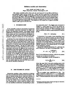
How does the CM model differ from the V AR in fitting yields? The answer lies in its spanning property. Panel A of Figure 1 reports the estimated loadings of yields (including the short rate) on the risk factor EX ,t in the US. The left panel shows the loadings on the inflation conditional mean, and the right panel shows the loadings 17

In contrast, Chernov and Mueller (2011) mention (but do not report results) that 4-factor models have trouble matching yield and survey data, with yield errors increasing three- to five-fold. The need to include an additional factor may arise because of their inclusion of long-horizon survey forecasts, or the much longer sample period.

22

on the unemployment rate conditional mean. These loadings are essentially zero for the V AR. This result is consistent with model T 3 in Chun (2011), combining two yield factors and inflation survey forecasts. He finds small loadings on expected inflation. In other words, the conditional means of macro variables are unspanned by nominal yields in these models. This was not pre-ordained: we did not impose spanning restrictions on the conditional means at estimation. For the V AR model, this is not unexpected either. Section 2.1 shows that much of the variation in the macro variables is unrelated to variations in the yields. The CM model paints a very different picture. The short-rate coefficients for the expected inflation and expected unemployment are 1.16 and -0.36, respectively. The pattern of loadings across maturities indicates that the level of yield rises but that its slope flattens when expected inflation increases. The loading on expected inflation decreases to 0.61 for the 10-year bond. Similarly, the pattern of loadings indicates that the level increases and the slope flattens when expected unemployment decreases. Panel B shows that the loadings for Canadian yields exhibit the same pattern. If anything, the influence of macro variables on yields is larger in the Canadian data, yet the yield loadings on the macro conditional means remain close to zero in the V AR.

4.3

forecasting inflation

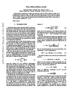
Figure 2 shows the expected inflation at horizons of 3 months, 1 year, and 2 years from the CM model. Panels A and (B) reports the results for the US and for Canada, respectively. Expected inflation is strongly procyclical and declines from 3% early in the sample to around 2% in 2004 in the US and in 1994 for Canada. Figure 2 also shows that the slope of expected inflation changes sign over time. Short-run inflation expectations stand above long-run inflation expectations when unemployment is high. The slope has been negative in the US since 2008. Yields should span conditional means in CM models. This requires that forecasts from the model should be as good as any other forecasts. Ang, Bekaert, and Wei (2007) argue that surveys provide the most accurate inflation forecasts (see also the survey by Faust and Wright 2011). We check that the CM model provides valid conditional expectations, using survey forecasts as a benchmark. We first estimate the models with data until December 1991, producing inflation forecasts that correspond 23

to each survey forecast at the end of that month. For this purpose, we extend the sample back to 1985 in Canada. We then add one month to the estimation sample, produce new inflation forecasts, and repeat until the end of 2012. At each date, we also produce forecasts of the annualized inflation rate for horizons between 1 and 24 months ahead. 4.3.1 Matching survey forecast accuracy Table V reports the ratio of the inflation forecast RMSEs from the models relative to the forecast RMSEs from the survey. Panels A and (B) report results for US and Canadian inflation forecasts, respectively. No model systematically improves upon the accuracy of survey forecasts, but most models perform reasonably well. In contrast to Ang, Bekaert, and Wei (2007), we find that the V AR and CM models match the accuracy of surveys, confirming the spanning assumption. The pattern is consistent across countries. While each model offers similar forecast accuracy when survey data are available, we show below that forecasts from the CM are superior when survey data are unavailable. Finally, note that conditional mean spanning requires ratios close to one but not necessarily equal to one. Survey participants and bond investors do not have and do not report the same conditional forecasts for future inflation. 4.3.2 Using survey data at estimation The model-implied inflation forecasts are accurate because estimation uses the likelihood of survey inflation forecasts. Panel A of Figure 3 reports the ratios of inflation forecast RMSEs from models estimated using the full likelihood relative to that from models estimated excluding the likelihood of survey data (Case A relative to Case C). Panel A reports RMSE ratios for US and Canadian data. The impact of the survey data is apparent. The forecast RMSEs deteriorate by 5-10% for 1-year forecasts in US data, and by as much as 20-25% for 2-year forecasts. The effect is typically larger in Canadian data. The deterioration is more severe for the CM models, except in Canadian data for the longer horizons. This pattern reflects this model’s larger parameterization. The likelihood of survey data plays a more important role as the number of parameters increases, in effect mitigating the loss in parsimony. To summarize, estimates that neglect survey data suffer from substantial bias and small-sample sampling errors. Adding surveys to the likelihood effectively lengthens the sample (Kim, 2007; Kim and Orphanides, 2012). Ang, Bekaert, and Wei (2007) find that survey forecasts are more accurate than model-based forecasts, but they do 24

not use survey data at estimation.18 4.3.3 Using the Markovian restriction The Markovian restriction makes inflation forecasts less accurate. Panel B of Figure 3 reports the ratio of forecast RMSEs from CM models relative to that from V AR models. Panel B reports results for the US and Canada, using all the available data or excluding the survey data (Cases A and B). For the US, the CM model yields accuracy improvements of 5% at the 1-year horizon and nearly 10% at the 2year horizon (significant at the 1% level), but the CM model yields no improvement in Case B. In Canada, the improvements are remarkable. The CM model produces accuracy gains in the 20-25% range at the 1-year and 2-year horizons. How can every model perform similarly when compared to survey forecasts (Table V), while the CM model outperforms when compared to the V AR? First, survey forecasts are available only quarterly in Canada, and the comparison with model forecasts can be done only quarterly. However, the comparison between models is done with monthly data. We find that forecast errors from the V AR models are also more serially correlated: this model performs relatively poorly in months when survey forecasts are not available. But survey forecasts are available monthly in the US. The forecasting horizons also drive the contrasting results. The comparison with survey forecasts involves forecasts for inflation in specific quarters. On the other hand, the comparison between models involves forecasts of total inflation between now and some future horizon h-months ahead. These horizons are relevant, since they are used in the yield decomposition below. The RMSEs between these two horizons can only differ because of the covariance between the forecast errors across quarters. Indeed, we find that forecast errors from the V AR models are more correlated across horizons (unreported). 18

It is essential to include yield factors in state Xt to match the accuracy of survey inflation forecasts. Results are available from the authors.

25

4.4

why conditional mean models for inflation forecasts?

How does a conditional mean model offer more accurate forecasts? To answer this question, consider the V AR model, VAR:

EX ,t = K0X + (K1X + INZ )Xt = K0X + (K1X + INZ )EX ,t−1 + (K1X + INZ )(Xt − EX ,t−1 ) = K0X + (K1X + INZ )EX ,t−1 + (K1X + INZ )uX ,t ,

(43)

with uX ,t ≡ (Xt − EX ,t−1 ), and contrast with the CM model, CM:

EX ,t = K0X + (K1X + INZ )EX ,t−1 + ΣEX ǫPt = K0X + (K1X + INZ )EX ,t−1 + ΣEX Σ−1 X (Xt − EX ,t−1 ) = K0X + (K1X + INZ )EX ,t−1 + ΣEX Σ−1 X uX ,t ,

(44)

where the weights (K1X + INZ ) on the prior expectations EX ,t−1 can differ from the weights ΣEX Σ−1 X on the innovations uX ,t . Tables VI-VII report parameter estimates for the US and for Canada, respectively. In each case, Panel A reports estimates of the matrices K1X + INZ and ΣEX Σ−1 X . Panel B reports estimates of the standard deviations (on the diagonals) and the correlations (off the diagonals) implied from the estimate of the covariance matrix ΣX Σ′X and ΣEX Σ′EX . Focusing on the first line of (K1X + INZ ) and ΣEX Σ−1 X , the estimated dynamics of inflation expectations Eπ,t = Et [πt+1 ] illustrate the difference: Eπ,t = 0.98 × Eπ,t−1 − 0.01 × uπ,t − 0.04 × Eg,t−1 + 0.51 × ug,t (0.03)

(0.001)

(0.02)

(0.06)

+ 0.008 × El,t−1 + 0.01 × ul,t − 0.02 × Es,t−1 + 0.02 × us,t, (0.003)

(0.01)

(0.02)

(0.04)

(45)

and, again, we have very similar results in the case of Canada: Eπ,t = 1.03 × Eπ,t−1 − 0.005 × uπ,t − 0.07 × Eg,t−1 + 0.35 × ug,t (0.15)

(0.002)

(0.06)

(0.07)

+ 0.003 × El,t−1 − 0.03 × ul,t − 0.04 × Es,t−1 + 0.26 × us,t , (0.003)

(0.01)

(0.04)

26

(0.06)

(46)

with standard errors provided in parentheses.19 First, expected inflation is very persistent in both countries: inflation innovations are transitory and have close to no effect on the expectation update. Also, note from Tables VI and VII that inflation innovations have no significant effect on El,t and Es,t , while their effect on Eg,t is small (see the first column of ΣEX Σ−1 X ). Hence, the intuition from Kim (2007) that inflation combines a persistent conditional mean component with transitory noise (i.e., an ARMA(1,1) process) carries over in our multivariate context. The V AR cannot distinguish between these two components. Second, updates of expected inflation are driven by innovations in the other variables since the coefficient on inflation innovation is almost zero (albeit significant in Canada). The CM model uses the span of uX ,t to capture predictable variations in expected inflation. Multiplying coefficients by the corresponding standard deviation shows that unemployment innovations are the most significant economically (standard deviation of 0.26). Slope innovations also play an important role in Canada (standard deviation of 0.45). In contrast, unemployment and slope innovations are only weakly connected to expected inflation updates in the V AR model (unreported). Third, the estimated weights on the prior expectations differ from the estimated weights on the innovations in every case, and with opposite signs in every case. Expected inflation increases with a higher expected level of the yield curve, but shows no response to surprise changes in the level. Expected inflation increases with an expected rise in the slope, but decreases with a surprise tightening of the short rate. An increase of st lifts short-maturity yields relative to longer maturities, and corresponds to a tighter stance of monetary policy. Expected inflation also decreases with a higher expected unemployment rate but increases with a surprise increase in the unemployment rate. The V AR must assign the same weight and sign to the innovation and the expectation terms. Inspecting the estimate for ΣEX Σ′EX reveals the correlation between the updates of different conditional means. In the US, the update of expected inflation is positively correlated with an update in expected unemployment and with an update in the slope factor. It is also negatively correlated with an expected increase in the level of yields. This effect is not statistically significant. Therefore, a standard expectation update sees higher expected inflation, a flatter expected curve (the slope factor pushes 19

ˆ 1X + INZ has no unit root in both cases. The autoregressive matrix K

27

short-maturity yields up), and higher expected unemployment. In contrast, inflation innovations are uncorrelated with unexpected unemployment changes. In Canada, a standard expectation update also sees higher expected inflation, a flatter expected curve and higher expected unemployment. However, the correlation with the expected level of yield is stronger in Canada. In addition, inflation innovations exhibit a low correlation with other innovations: monthly inflation appears largely unpredictable in Canada. Again, the V AR cannot capture these separate effects.

4.5

nominal yield decompositions

4.5.1 Fisher’s decomposition Real yields are identified within the model if the expected inflation and the inflation-risk premium can be derived from the model. Hence, if the inflation rate is included in the P-dynamics, and if the inflation-risk premium is identified, it follows that real yields are identified. The only additional assumption is the absence of an arbitrage opportunity in the real bond market. The real short rate rt follows from the link between the nominal and the real stochastic discount factors, SDFt+1 and r r SDFt+1 , respectively. This link, SDFt+1 ≡ e−it ξt+1 = e−πt+1 SDFt+1 , implies that


1 r rt ≡ − log Et [SDFt+1 ] = it − EtQ [πt+1 ] − σπ2 , 2

(47)

where σπ2 ≡ V art [πt+1 ]. This definition corresponds to Fisher’s decomposition, but where the expectation EtQ [πt+1 ] is taken under the risk-neutral measure. Using Equation (24), the real short rate can be written analogously to the nominal rate, rt = ρr0X + ρr′ 1X EX ,t ,

(48)

and it follows that real yields are given by (n)

rt

= ar,n + b′r,n EX ,t ,

(49)

with the coefficients ρr0X and ρr1X and the loadings ar,n and br,n given in Appendix A1. For longer-maturity yields, we have the following generalized Fisher decomposition: (n)

it

(n)

≡ c(n) + rt

(n)

(n)

+ Eπ,t + irpt ,

28

(50)

(n)

(n)

(n)

where rt is the n-period real yield, irpt is the inflation-risk premium, Eπ,t is the inflation expectation, and c(n) is a Jensen term (see Appendix A5). 4.5.2 Inflation swaps, risk premium, and Sharpe ratio Real yields may be imprecisely estimated even if formally identified, and using inflation swap rates helps pin down the decomposition in the US. However, the additional data are not reliably available in most countries (Canada is a typical case). To improve estimates of the real yield in these cases, we constrain the inflation Sharpe ratio within a plausible area of the parameter space (see Section 3.2.6). We ask if the inflation-risk premium estimates are similar whether we use inflation swaps at estimation or exclude them. To check this, we re-estimate the CM model with US data, excluding the inflation swaps from the joint likelihood (Case B), but using the same constraint on the conditional Sharpe ratio as in the case of Canada. We focus on the subsample where US markets were relatively unaffected by liquidity shocks and policy intervention. The financial crisis and the rounds of quantitative easing introduce a wedge between the risk premium implicit in Treasury yields and the risk premium implicit in the inflation swaps (Krishnamurthy and Vissing-Jorgensen, 2011; Fleckenstein, Longstaff, and Lustig, 2013). Estimates based om post-2007 will reflect that wedge. Therefore, we proceed with data between 1985 and 2007. Figure 4 compares the model-implied and observed inflation swap rates for 2-, 5-, and 10-year maturities, and extends the estimation sample until 2012. The swap rates predicted from the model are close to the observed rates. In fact, excluding the swap data seems to help in the crisis. The model-implied rates do not plunge like observed rates do (as low as -2% in the case of the 2-year swap). This must be assessed as a benefit of using the Sharpe ratio constraint. The model-implied and observed rates then remain close to each other until the end of 2010, which coincides with the second round of quantitative easing. At this point, the model-implied rates follow nominal yields, slowly drifting downward, while inflation swap rates remain high. The wedge between the model and the swap markets is similar across maturities (note the different scales). Including the swap data is beneficial in this case. Overall, the results suggest that bounding the inflation Sharpe ratio is a close substitute to using the inflation swap data. Figure 5 illustrates the impact of the Sharpe ratio constraint on the yield decomposition in Canada. Panel A shows the 2- and 5-year inflation-risk premium obtained 29

when the Sharpe ratio is unconstrained. Panel B shows the results with the constraint set to κ = 0.2.20 The excess variability of the inflation-risk premium stands out in the unconstrained case: the 2-year inflation-risk premium varies between -20% and 5%, and the 5-year inflation-risk premium varies between -5% and 15%! These large values imply implausibly large variations in the real yields. In contrast, the constrained model produces estimates of the inflation-risk premium that are economically plausible and close to the US estimates, ranging between 0% and 2%. 4.5.3 Fisher’s decomposition in CM and V AR models This section assesses how the decomposition of US nominal yields changes as the information set used for estimation changes. We report results for the 2-year yield from the CM and the V AR models across Cases A and C. The yield decompositions are very similar across estimates of the CM model, but the estimates vary across V AR models. The left column of Figure 6 reports results for the CM model. The path of 2-year expected inflation is very similar across cases. The estimated inflation-risk premium becomes more volatile when we add inflation swap data. This reflects the fact that we do not enforce the constraint on the Sharpe ratio in this case. Also, the inflation-risk premium rises in 2011 and 2013. As noted in Section 4.5.2, unconventional policies introduce a wedge between nominal yields and inflation swaps. Otherwise, the results are remarkably similar. The right column of Figure 6 reports results for the V AR model. The message could not be more different. The estimates of the inflation-risk premium become erratic when we exclude the inflation swap. Even when we include all the data, in Case A, the estimates of the inflation-risk premium differ from the CM model, reflecting the poor fit of the swap data documented in Table IIIA. Results from the V AR are not reliable. 20

We assess the variability of several other model properties as we vary κ. The short-rate loadings, yield loadings, measurement errors, and forecasting performance remain essentially unchanged for values of κ around 0.2. However, the likelihood increases monotonically as we increase κ to implausible values, and with very little improvement in pricing errors – a telling tale of overfitting. The risk premium variability also increases monotonically. Results are available from the authors.

30

4.5.4 Nominal yield decomposition in the US and Canada Figure 7 compares the decompositions from our benchmark model in the US and in Canada.21 It displays the 2-year nominal yield, expected inflation, and inflationrisk premium. Panel A reports the decomposition in the US, reproducing the results from Figure 6A. Panel B reports the decomposition the Canada. For the reasons discussed in Section 4.5.2, we use parameters estimated with data until 2007 for the US. Looking beyond the cyclical variations, we see that the inflation-risk premium in both countries had been drifting down until 2008, from around 1% to around 0% in the US and from 2% to 0% in Canada. The inflation-risk premium is procyclical in the US, rising when nominal yields rise, and dampening the transmission of interest rate shocks to the real curve. Real yields are less cyclical than nominal yields in the US. This is consistent with results in, for example, Chernov and Mueller (2011).22 In contrast, the inflation-risk premium is counter-cyclical in Canada, amplifying the transmission of interest rate shocks to the real curve. Real yields are more cyclical than nominal yields in Canada. This stark difference between the two countries may arise because of the different mandates given to their respective central banks. The Bank of Canada has had an explicit inflation target since the beginning of our sample, but the Fed has had a dual mandate, weighting employment and inflation targets. We leave the causal mechanism underlying this difference to future research, but the results suggest that monetary policy achieves a greater bang for the buck in Canada. This difference implies a very different response of the inflation-risk premium to the large declines of long-term yields in both countries since 2009. In the US, the modelimplied premium followed the decline in yields during the crisis and has remained between -1.5% and -2.0% since then. Exposures to inflation risk are perceived as hedges by US bond investors. In contrast, the inflation-risk premium increased to 1% between 2009 and 2010 in Canada and has remained elevated since. Exposures to inflation shocks are perceived as risky by Canadian bond investors. Again, the 21

These are the first real yield estimates for Canada. Ragan (1995) is an early attempt to measure expected inflation from nominal yields in Canada. Day and Lange (1997) provide time-series evidence that the term spread has predictive content for inflation rates in Canada. Fung, Mittnick, and Remolona (1999) study a joint model for the US and Canadian term structures. They do not use survey data to identify inflation expectations. Garcia and Luger (2007) estimate an equilibriumbased model for yields in Canadian data where conditional expectations play a central role. 22 See the results for “AO5” models in their Figure 4.

31

difference may be linked to the difference between the Fed’s and the Bank of Canada’s mandate. The Fed may be perceived to accommodate inflation shocks to fulfill its dual mandate, as least in the early stage of an expansion, while the Bank of Canada may be perceived to effectively counter inflation shocks. This interpretation is consistent with the lower volatility of expected inflation between the US and Canada in Figure 2. David and Veronesi (2013) provide empirical evidence that inflation shocks can be good news and bad news in the context of a general equilibrium. This effect may also arise with Epstein-Zin preferences: inflation may signal higher consumption growth, leading to upward revisions for utility value (through the continuation value). Table VIII reports sample summary statistics for each component of nominal yield in Canada, and for maturities of 3 and 6 months, as well as 1, 2, 5, and 10 years. We focus on the case of Canada since summary statistics for the US nominal yields have been documented elsewhere. The average nominal yield curve is upward sloping – the slope between 3-month and 10-year yields averages close to 1.3% in our sample – but the curve exhibits significant variability throughout the cycle: the average volatility ranges from 3.28% to 2.44%. Real yields are downward sloping – the average slope is -0.7% – suggesting that investors perceive real bonds as hedges in Canada. The average expected inflation is flat, above 2%. Therefore, the average positive slope of nominal yields is due to the slope of the inflation-risk premium. The inflation-risk premium average ranges from almost zero at the shortest maturity to 1.6% at the 10-year maturity.

5.

Conclusion

We introduce the class of CM-MTSMs where the conditional mean Et drives the term (n) structure of yields yt = an + b′n Et as well as the dynamics of the state variables. The essence of our approach is the departure from the Markov assumption: Et depend on the entire history of Zt . This extension is parsimonious and gives fundamentally different roles to Zt , which captures the current state, and to Et , which summarizes yields as well as the conditional mean of Zt+1 . Including inflation within a CMMTSM as a showcase, the results illustrate the distinctive properties of CM-MTSMs: (i) yields span expected inflation as measured by survey forecasts, and (ii) expected changes and surprises in unemployment and in the level or the slope have opposite effects on inflation expectations. A simpler Markovian VAR(1) model does not capture 32

these features. In addition, our approach reconciles models using survey forecasts as state variables with models using the underlying macro variables as state variables. Importantly, including survey data overcomes the effect of sampling variability on the estimates of persistence parameters, and including inflation swap data helps us obtain plausible estimates of the inflation-risk premium, but estimates of the CM remain robust when the additional data are not available for estimation. The dynamics in CM-MTSMs are consistent with several general-equilibrium specifications where the observable macro variables are not Markovian (e.g., Bansal and Yaron 2004; Bansal and Shaliastovich 2013). Our results suggest that (nonMarkovian) long-run risk models with a structural pricing kernel calibrated to reasonable Sharpe ratio may fit term structure data (e.g., Bansal and Shaliastovich 2013). In that context, our results raise the question as to why inflation shocks may be perceived as a hedge in the US since 2009, but perceived as a risk in Canada. We also leave important extensions for future research. First, we focus on relatively short horizons, of less than 10 years. Kozicki and Tinsley (2001, 2006) highlight the role of shifting endpoints in the evolution of long-horizon inflation rates in US data. In Canada, Amano and Murchison (2006) show the importance of a shifting endpoint for inflation in the early 1990s during the transition toward a 2% inflation-targeting regime. Second, we focus on inflation forecasts, but forecasts of future inflation rates are not independent of forecasts of other macro forecasts. Extending our approach to include additional variables, such as unemployment, could help identify the dynamic relationships between economic activity, inflation, and risk as perceived by bond investors. The framework proposed here can be extended in these directions.

33

A

Appendix

A1

yield coefficient recursions

The price of a nominal zero-coupon bond with maturity n is given by D(t, n) = exp (An + Bn′ Et ) with coefficients given by Bn+1 =(INZ + K1Q′ )Bn − ρ1 1 An+1 =An + K0Q′ Bn + Bn′ ΣE Σ′E Bn − ρ0 , 2

(A.1)

for n > 0 and with initial conditions A0 = 0 and B0 = 0. The nominal yield coefficients are given by an ≡ −An /n and bn ≡ −Bn /n. From Equations (24) and (47), it follows that the real rate coefficients in Equation (48) are given by   1 Q P − K K ρr0X ≡ ρ0X − σπ2 − e′1 ΣX Σ−1 0X 0X EX 2 i′  h Q P e1 . ρr1X ≡ ρ1X − e1 − ΣX Σ−1 EX K1X − K1X

A2

(A.2)

risk premium

From Equations (8), (13), and (12), it follows that EtQ ≡ EtQ [Zt+1 ] = Et + ΣEtQ [ǫPt+1 ] Q P P = Et + ΣΣ−1 E Et [∆Et+1 − K0 − K1 Et ]   Q Q P P K − K E − K − K E = Et + ΣΣ−1 t t 0 1 0 1 E     Q Q P −1 P EtP . K − K + ΣΣ K − K = Et + ΣΣ−1 1 0 1 0 E E

A3

(A.3)

proposition 2

The NZ × 1 vector of observable Xt defined in Equations (19)–(20) has the same dynamics as the process for Zt . We define D:   (A.4) D ≡ D1 + D2 K1P + INZ ,

34

and we require that D be invertible. Using the mapping between Xt and Zt given in Equation (19), the parameters for the dynamics of Xt are given by   P K0X =DK0P − DK1P D −1 C + D2 K0P P K1X =DK1P D −1

(A.5)

  Q K0X =DK0Q − DK1Q D −1 C + D2 K0P

Q =DK1Q D −1 K1X

(A.6)

ΣEX =DΣE ΣX =D1 Σ + D2 ΣE .

A4

(A.7)

theorem 1

The canonical form for Zt in Proposition 1 is exactly identified. We verify that the parameterization for Xt in Theorem 1 is also identified. First, we redefine D in Equation (A.4) to substitute out
the matrix K1P , which belongs to the dynamics of Zt . Given D ≡ D1 + D2 K1P + INZ and using P = DK P D −1 from Proposition 2, it follows that K1X 1   D =D1 + D2 K1P + INZ P =D1 + D2 + D2 D −1 K1X D,

(A.8)

where D1 and D2 are defined in Equation (20). Rearranging: P IN = (D1 + D2 ) D −1 + D2 D −1 K1X  
P vec (IN ) = vec (D1 + D2 ) D −1 + vec D2 D −1 K1X 

 P′ ⊗ D2 vec D −1 , vec (IN ) = (IN ⊗ (D1 + D2 )) vec D −1 + K1X

(A.9)

and, therefore, D is defined implicitly by    
P′ ⊗ D2 vec D −1 = vec (IN ) . IN ⊗ D1 + IN + K1X

We require that



   P′ ⊗ D2 INZ ⊗ D1 + INZ + K1X

(A.10)

be invertible so that D −1 is well-defined. Second, we explicitly provide the mappings between the parameters of Zt and the parameters of Xt . The mapping between the P parameters is given by −1    P P P K0X + K1X C K0P = D − K1X D2 P K1P =D −1 K1X D

ΣE =D −1 ΣEX D1 Σ =ΣX − D2 D −1 ΣEX ,

35

(A.11)

and the mapping for the Q parameters is given by     Q P K0X = DK0Q − DJ λQ (D1 + D2 )−1 C + D2 D −1 K0X   Q K1X = DJ λQ D −1 .

(A.12)

See Proposition 1. Importantly, both sides of the last equation in (A.11) have the same rank as D1 , which cannot be inverted since its lower block is zero. In other words, we cannot identify ΣX and ΣEX separately whenever yield portfolios are included among the observable variables. To complete the parameterization in the theorem, rewrite  ∗ Σ , (A.13) D1 Σ = 0 defining Σ∗ implicitly. Then, ΣX is given by the last equation in (A.11) in terms of the other parameters,  ∗ Σ . (A.14) ΣX = D2 D −1 ΣEX + 0 Turning to the short rate, from Equations (19)–(20) and Proposition 1, it follows that the coefficients in Equation (21) are given by   P ′ ρ0X = − ı C + D2 K0 ρ′1X =ı′ D −1 .

(A.15)

The dynamics of Xt in Equations (22)–(23) follow from Proposition 2. Finally, the spread between EXQ,t and EXP ,t in Equation (24) follows from Proposition 2 and Equation (17).

A5

Generalized Fisher Decomposition

The generalized Fisher decomposition can be applied to any nominal yield with maturity n, (n)

it (n)

where rt

(n)

≡ c(n) + rt

(n)

+ irpt ,

(n)

is the n-period-ahead inflation risk premium,      n n X 1  Q X ≡ Et πt+j  − Et  πt+j  , n

is the real yield, and irpt (n)

irpt

j=1

π,(n)

where Et

π,(n)

+ Et

j=1

is the n-period-ahead inflation expectation, # " Pn π t+j j=1 π,(n) , ≡ EtP Et n

and where c(n) is a Jensen term, n−1


1 X 2 ′ 1 j br,j Σm Σ′m br,j − b′j Σm Σ′m bj . c(n) = σπ2 + 2 2n j=0

36

(A.16)

A6

combining inflation and survey inflation forecasts

Rearrange the vector Mt of macroeconomic variables as Mt = [Ot′ St′ ]′ where Ot stacks the macro data (i.e., the inflation rate) and St stacks the corresponding survey data (i.e, the inflation survey). As before, the observed variables are linked to the latent factors as in Equation (18), ′ Ot = γ0O + γO Zt

St = γ0S + γS′ Et ,

(A.17)

but changing the notation slightly. We derive parametric restrictions such that we have St = EtP [Ot+1 ] + ηt

(A.18)

where ηt is a measurement error: E[ηt ] = 0 and cov(ηt , ηt+h ) = 0 ∀h > 0. This implies restriction on the P-dynamics of Xt . Define Yt′ = [Xt′ EX′ ,t ] with dynamics given by Yt+1 = µY + φY Yt + ǫY,t ,

(A.19)

and parameters given by 

0 µy = P K0X





   0 I 0 I φY = . P ) = 0 φ 0 (I + K1X X

(A.20)

Define e′O and e′S such that e′O Xt = Ot and e′S Xt = St . Then, ηt = e′S Xt − e′O EX ,t = β ′ Yt with β ′ ≡ [e′S − e′O ] and, therefore, cov(ηt , ηt+h ) is given by   0 0 cov(β ′ Yt , β ′ Yt+h ) = β ′ cov(Yt , Yt+h )β = β ′ ΩY (φ′Y )h β = β ′ ΩY β ∀h > 1, (φ′X )h−1 (φ′X )h−1 (A.21) where we define the following implicitly:     var(Xt ) cov(Xt , EX ,t ) ΩX ΩXE ΩY ≡ ≡ . (A.22) cov(EX ,t , Xt ) var(EX ,t ) ΩEX ΩE Hence,

where we define


cov(ηt , ηt+h ) = e′S ΩXE − e′O ΩE (φ′X )h−1 δ, δ ≡ eS − φ′X eO .

(A.23)

(A.24)

Clearly, δ = 0 ⇒ cov(ηt , ηt+h ) = 0 ∀h > 0, which is the condition that we discuss in the main text. Developing Equation (A.23), we can derive additional sufficient conditions. Tedious algebra yields
′ h−1 ′ ′ cov(ηt , ηt+h ) = δΩX φ′X + e′O θX Ωǫ φ′X − (δ + θX eO )′ Ωǫ θX (φX ) δ, (A.25) where θX = φX − ΣEX Σ−1 X . See also Section 2.6.5. Turning to the condition on the mean: E[ηt ] = 0 P E[β ′ Yt ] = β ′ (µy + φy E[Yt ]) = −e′O K0X + δ′ E[Yt ] = 0.

37

(A.26)

Then, neglecting conditions involving restrictions on the covariance matrix, the following condition implies that ηt is a measurement error: P δ = 0 and e′O K0X = 0.

(A.27)

These restrictions deliver a process where the consistency condition between expectation and survey data holds, but the canonical form in Theorem 1 must be adapted (available from the authors). If, in addition, γ0O = γ0S and γO = γS , then the canonical form in Theorem 1 follows through but using the relabeled coefficients γ0O and γO instead of γ0 and γ1 . We modify Equation (18) as follows: Mt = γ0 + γ1 Zt + γ2 Et , (A.28) with loadings given by



γ γ0 = 0O γ0S





γ γ1 = O 0





 0 γ2 = . γS

(A.29)

Then, these additional restrictions on the matrix C, D1 , and D2 are given by e′O C = e′S C = γπ0 e′O D1 = e′S D2 = γπ′ e′S D1 = e′O D2 = 0 This implies that P e′O K0X =0

P e′O (I + K1X ) = e′S

e′O θX = 0,

(A.30)

P = 0. From and, in addition, that var(ηt ) = 0 (no measurement error). First consider e′O K0X Equation (A.5),     P P C + D2 K0P γπ′ K0P − (eS − eO )′ C + D2 K0P e′O K0X =e′O DK0P − e′O K1X

=γπ′ K0P − (eS − eO )′ C + (eS − eO )′ D2 K0P γπ′ K0P − 0 + γπ′ K0P = 0,

(A.31)


′ P = e′ − e′ . Note that e′ D = e′ (D + D K P + I where we used K1X 1 2 NZ ) = γπ . Then, 1 X O O O P P −1 P −1 P −1 e′O K1X =e′O DKX D = γπ′ KX D = e′S D2 KX D

=e′S (D − D1 − D2 )D −1 = e′S (INZ − D1 D −1 − D2 D −1 ) =e′S − 0 − e′S D2 D −1 = e′S − γπ′ D −1 = e′S − e′O .

(A.32)

Finally, P St = e′S Xt = e′O EX ,t = e′O I + K1X + eO θX EX ,t−1

= e′S Xt + eO θX EX ,t−1 St = St + eO θX EX ,t−1 ,

(A.33)

which can be true only if eO θX = 0. This in turn implies that e′O ΣEX = e′S ΣX and therefore that e′S Σ∗ = 0.

38

References Ajello, A., L. Benzoni, and O. Chyruk, 2012, Core and “crust”: Consumer prices and the term structure of interest rates, Federal Reserve Bank of Chicago. Amano, R., and S. Murchison, 2006, Factor-market structure, shifting inflation targets, and the new keynesian Phillips curve, in Issues in Inflation Targeting . pp. 89–109 (Bank of Canada). Ang, A., G. Bekaert, and M. Wei, 2007, Do macro variables, asset markets, or surveys forecast inflation better?, Journal of Monetary Economics 54, 1163–1212. , 2008, The term structure of real rates and expected inflation, The Journal of Finance 63, 797–849. Ang, A., S. Dong, and M. Piazzesi, 2007, No-arbitrage Taylor rules, Working paper 13448 National Bureau of Economic Research. Ang, A., M. Piazzesi, and M. Wei, 2006, What does the yield curve tell us about GDP growth?, Journal of Econometrics 131, 359–403. Bansal, R., and I. Shaliastovich, 2013, A long-run risks explanation of predictability puzzles in bond and currency markets, Review of Financial Studies 26, 1–33. Bansal, R., and A. Yaron, 2004, Risks for the long run: A potential resolution of asset pricing puzzles, The Journal of Finance 59, 1481–1509. Bauer, G., and A. Diez de los Rios, 2012, An international dynamic term structure model with economic restrictions and unspanned risks, Working paper 2012-5 Bank of Canada. Bauer, Michael D., Glenn D. Rudebusch, and Jing Cynthia Wu, 2012, Correcting estimation bias in dynamic term structure models, Journal of Business and Economics Statistics 30, 454–467. Campbell, J. Y., R. J. Shiller, and LUIS M. Viceira, 2009, Understanding inflation-indexed bond markets, Brookings Papers on Economic Activity 2009, 79–120. Chen, R.R., B. Liu, and X. Cheng, 2010, Pricing the term structure of inflation risk premia: Theory and evidence from TIPS, Journal of Empirical Finance 17, 702–721. Chernov, M., and P. Mueller, 2011, The term structure of inflation expectations, Journal of Financial Economics 106, 367–394. Christensen, J. H. E., J.A. Lopez, and G.D. Rudebusch, 2010, Inflation expectations and risk premiums in an arbitrage-free model of nominal and real bond yields, Journal of Money, Credit and Banking 42, 143–178. Chun, A. L., 2011, Expectations, bond yields, and monetary policy, Review of Financial Studies 24, 208–247.

39

D’amico, S.D., D.H. Kim, and M. Wei, 2010, Tips from TIPS: The informational content of Treasury infation-protected security prices, Working paper 2010-10 Federal Reserve Board. David, A., and P. Veronesi, 2013, What ties return volatilities to price valuations and fundamentals?, The Journal of Political Economy 121, 682–746. Day, J., and R. Lange, 1997, The structure of interest rates in Canada: Information content about medium-term inflation, Working paper 97-10 Bank of Canada. Duffee, G., 2010, Sharpe ratios in term structure models, Working paper Johns Hopkins University. , 2011, Information in (and not in) the term structure, Review of Financial Studies 24, 2895–2934. Faust, J., and J. Wright, 2011, Forecasting Inflation . in Handbook of Economic Forecasting (Elsevier). Fernandez-Villaverde, J., J.F. Rubio-Ramirez, and T. Sargent, 2005, A,B,C’s (and D’s) for understanding VARs, Working Paper 05-018 Penn Institute for Economic Research. Feunou, B., and N. Meddahi, 2007, Generalized affine models, Working Paper Universit´e de Montr´eal. Fiorentini, Gabriele, and Enrique Sentana, 1998, Conditional means of time series processes and time series processes for conditional means, International Economic Review 39, 1101– 1118. Fisher, I., 1930, The theory of interest (New York: The Macmillan Co.). Fleckenstein, Matthias, Francis A. Longstaff, and Hanno Lustig, 2013, The TIPS-Treasury bond puzzle, The Journal of Finance p. forthcoming. Friedman, M., 1968, The role of monetary policy, American Economic Review 58, 1–17. Fung, B.S.C., S. Mittnick, and E. Remolona, 1999, Uncovering inflation expectations and risk premiums from internationally integrated financial markets, Working paper 99-6 Bank of Canada. Garcia, R., and R. Luger, 2007, The Canadian macroeconomy and the yield curve: an equilibrium-based approach, Canadian Journal of Economics 40, 561–583. Gurkaynak, R.F., B. Sack, and J.H. Wright, 2006, The U.S. Treasury curve: 1961 to present, Working paper 2006-28 Federal Reserve Board. Hasseltoft, H., 2012, Stocks, bonds, and long-run consumption risks, Journal of Financial and Quantitative Analysis 47, 309–332.

40

Haubrich, J., G. Pennacchi, and P. Ritchken, 2012, Inflation expectations, real rates, and risk premia: Evidence from inflation swaps, Review of Financial Studies 25, 1588–1629. Jardet, C., A. Monfort, and F. Pegoraro, 2013, No-arbitrage near-cointegrated VAR(p) term structure models, term premia and GDP growth, Journal of Banking and Finance 37, 389–402. Joslin, S., A. Le, and K. H. Singleton, 2013a, Why Gaussian macro-finance term structure models are (nearly) unconstrained factor-VARs, Discussion Paper, 3. Joslin, Scott, Anh Le, and Kenneth J. Singleton, 2013b, JFEC invited paper: Gaussian macro-finance term structure models with lags, Journal of Financial Econometrics 11, 581–609. Joslin, S., M. Priebsch, and K. J. Singleton, 2012, Risk premiums in dynamic term structure models with unspanned macro risks, The Journal of Finance (forthcoming). Joslin, S., K. J. Singleton, and H. Zhu, 2011, A new perspective on Gaussian dynamic term structure models, Review of Financial Studies 24, 926–970. Kim, Don H., 2007, Challenges in macro-finance modeling, Working paper BIS 240 Bank of International Settlements. Kim, D. H., and A. Orphanides, 2012, Term structure estimation with survey data on interest rate forecasts, Journal of Financial and Quantitative Analysis 47, 241–272. Kim, Don H., and J. H. Wright, 2005, An arbitrage-free three-factor term structure model and the distant-horizon forward rates, Working paper 2005–33 Board of Governors of the Federal Reserve System. Kozicki, S., and P.A. Tinsley, 2001, Shifting endpoints in the term structure of interest rates, Journal of Monetary Economics 47, 613–652. , 2006, Survey-based estimates of the term structure of expected U.S. inflation, Working paper 2006-46 Bank of Canada. Krishnamurthy, A., and J. Vissing-Jorgensen, 2011, The effects of quantitative easing on interest rates: Channels and implications for policy, Working paper NBER W17555. Mankiw, N.G., R. Reis, and J. Wolfers, 2003, NBER Macroeconomics Annual . chap. Disagreement about expected inflation, pp. 209–270 (MIT Press). Monfort, A., and F. Pegoraro, 2007, Switching VARMA term structure models, Journal of Financial Econometrics 5, 105–153. Pennacchi, GG, 1991, Identifying the dynamics of real interest rates and inflation: Evidence using survey data, Review of Financial Studies 4, 53–86. Phelps, E. D., 1967, Phillips curves, expectations of inflation and optimal employment over time., Economica 34, 254281. 41

Piazzesi, M., 2005, Affine term structure modelschap. 12 . in Handbook of Financial Econometrics (Elsevier). , and E. Schneider, 2006, Equilibrium yield curves, Working paper 12609 NBER. , 2009, Trend and cycle in bond premia, Working paper Stanford University. Ragan, C., 1995, Deriving agents’ inflation forecasts from the term structure of interest rates, Working paper 95-1 Bank of Canada. Ravenna, F., 2007, Vector autoregressions and reduced form representations of DSGE models, Journal of Monetary Economics 54, 2048–2064.

42

Inflation

Unemployment

1.2

0.05

0 1 −0.05 0.8 −0.1 0.6

−0.15

−0.2

0.4

−0.25 0.2 −0.3 0

VAR SAM CM

−0.35

−0.2

2

4

6

8

−0.4

10

2

4

years

6

8

10

years

A– US nominal yield loadings on expected inflation (left) and on expected unemployment (right) Inflation

Unemployment

2

0.2

0.1 1.5

0

−0.1 1 −0.2

−0.3 0.5 −0.4

−0.5

0

−0.6

−0.5

2

4

6

8

−0.7

10

years

2

4

6

8

10

years

B– Canadian nominal yield loadings on expected inflation (left) and on expected unemployment (right)

Figure 1. Nominal Yield Loadings. Loadings of nominal yields on the conditional mean of inflation and on the conditional mean of unemployment from the benchmark CM model in the US (Panel A) and in Canada (Panel B).

43

4

4

3.5

3.5

3

3

2.5

2.5

2

2

1.5

3 months 1 year 2 years

1.5

3 months 1 year 2 years

1 92 93 94 95 96 97 98 99 00 01 02 03 04 05 06 07 08 09 10 11 12 13

1 92 93 94 95 96 97 98 99 00 01 02 03 04 05 06 07 08 09 10 11 12 13

A– US

B– Canada

Figure 2. Term structure of expected inflation. Expected inflation from the CM benchmark model, over the horizons 3 months, 1 year, and 2 years in the US (Panel A) and in Canada (Panel B). Monthly data from January 1992 to December 2012.

44

1,05

1,05 VAR

CMͲCanada

surveys

VARͲCanada

1

1

0,95

0,95 RMSERatios

RMSERatios

CM

0,9 0,85

surveysͲCanada

9

12 15 HORIZONS(months)

nosurveyͲCanada

0,9 0,85

0,8

0,8

0,75

0,75

0,7

nosurvey

0,7 1

3

6

9

12 15 HORIZONS(months)

18

21

24

A– With or without surveys

1

3

6

18

21

24

B– CM vs V AR

Figure 3. Out-of-sample inflation forecast. Ratios of forecast RMSEs. Panel A reports the RMSEs for a given model estimated with survey data relative to the same model estimated without survey data (Case A vs. Case C). Results are reported for the CM and the V AR models, both for US and Canadian data. Panel B reports the RMSEs for the CM model relative to the corresponding V AR model using all data. Results are reported cases with and without survey data (Case A and Case C), for US data and Canadian data, respectively. Monthly data. Estimation sample: 19851992. Out-of-sample: 1992-2012.

45

24 months

2 0 CM Swaps −2 2005

2006

2007

2008

2009

2010

2011

2012

2013

2010

2011

2012

2013

2010

2011

2012

2013

60 months 3 2 1 0 2005

CM Swaps 2006

2007

2008

2009 120 months

3 2.5 2 1.5 2005

CM Swaps 2006

2007

2008

2009

Figure 4. Inflation swap rates. Observed and model-implied inflation swap rates between 2005 and 2013. The model-implied values are computed from the benchmark CM model estimated using data until the end of 2007, excluding inflation swap data altogether (Case B), and bounding the distribution of the conditional inflation Sharpe ratio.

46

100

2−year 5−year

2.5 80 2

60 40

1.5

20 1

0 −20

0.5

−40 0 −60 2−year 5−year

−80 1992

1994

1996

1998

2000

2002

2004

2006

2008

2010

−0.5 2012

1992

A– Unconstrained Sharpe ratio

1994

1996

1998

2000

2002

2004

2006

2008

2010

2012

B– Constrained Sharpe ratio

Figure 5. Inflation-risk premiums and the Sharpe ratio constraint. The 2-year and 5-year inflation-risk premium in Canada from the CM model where the Sharpe ratio is unconstrained (Panel A) and where it is constrained with κ = 0.2 (Panel B).

47

10

8

10 Expected inflation Inflation risk premium Nominal yield

8

6

6

4

4

2

2

0

0

−2

−2

92 93 94 95 96 97 98 99 00 01 02 03 04 05 06 07 08 09 10 11 12 13

92 93 94 95 96 97 98 99 00 01 02 03 04 05 06 07 08 09 10 11 12 13

A– CM (Case A)

B– V AR (Case A)

10

8

Expected inflation Inflation risk premium Nominal yield

10 Expected inflation Inflation risk premium Nominal yield

8

6

6

4

4

2

2

0

0

−2

−2

Expected inflation Inflation risk premium Nominal yield

92 93 94 95 96 97 98 99 00 01 02 03 04 05 06 07 08 09 10 11 12 13

92 93 94 95 96 97 98 99 00 01 02 03 04 05 06 07 08 09 10 11 12 13

C– CM (Case B)

D– V AR (Case B)

Figure 6. Nominal yield decomposition. Decomposition of the 2-year nominal yields between January 1992 and December 2012 in the US from different estimates of the CM model (left column) and the V AR model (right column). Panels A and A report results for Case A estimated using yield, inflation swap, and survey inflation forecast data. Panels D and C report results for Case B, estimated excluding the swap data.

48

8

9 8

Expected inflation Inflation risk premium Nominal yield

6 7 6 4 5 2

4 3

0 2 1 −2

Expected inflation Inflation risk premium Nominal yield

0

−4 92 93 94 95 96 97 98 99 00 01 02 03 04 05 06 07 08 09 10 11 12 13

−1 1992

A– CM (US data)

1994

1996

1998

2000

2002

2004

2006

2008

2010

2012

B– CM (Canadian data)

Figure 7. Nominal yield decomposition. Decomposition of the 2-year nominal yields between January 1992 and December 2012 in the US (Panel A) and in Canada (Panel B). Results from the CM model estimated with yields, inflation swaps and inflation survey forecasts (Case A).

49

Table I. Spanning regressions Panels A and B: R2 s from contemporaneous regression of survey forecasts on principal components from yields. Survey forecasts cover the current quarter up to 4 quarters ahead, Q0, Q1, Q2, Q3, and Q4, respectively. We use vectors of principal components that include either one, two, three, or four principal components from yields, P C1,t , P C2,t , P C3,t , and P C4,t . Panels C and D: R2 s from similar regressions for quarterly all-item urban CPI inflation rate and quarterly unemployment rate. Monthly survey data from Blue Chip, Gurkaynak, Sack, and Wright yield data, 1985-2012. Panel B– Spanning unemployment forecasts

Panel A– Spanning CPI inflation forecasts Q0 Q1 Q2 Q3 Q4

P Ct,1 31.5 71.5 80.6 82.0 82.3

P Ct,2 31.7 71.5 81.1 83.6 85.3

P Ct,3 31.9 71.9 82.3 84.8 86.9

P Ct,4 32.2 73.3 83.6 86.4 88.2

Q0 Q1 Q2 Q3 Q4

Panel C– Spanning CPI inflation rate Obs.

P Ct,1 10.8

P Ct,2 11.4

P Ct,3 13.4

P Ct,1 7.6 8.4 8.5 8.2 7.5

P Ct,2 44.7 44.5 42.5 39.9 37.5

P Ct,3 49.9 50.9 50.3 48.5 46.3

P Ct,4 56.3 57.5 57.7 56.7 55.7

Panel D– Spanning unemployment rate

P Ct,4 13.4

Obs.

50

P Ct,1 7.8

P Ct,2 44.5

P Ct,3 50.6

P Ct,4 57.4

Table II. Measurement errors – US Yields Standard deviation of measurement errors in annualized percentage for US yields. Cases A-C include different measurement equations for estimation. Case A includes measurement equations for the yields, the inflation survey forecasts and the inflation swaps. Case B excludes the inflation swaps. Case C also excludes the inflation survey forecasts. Panels A and B report results for CM models and for V AR models, respectively. Monthly data 12/1984-12/2012. Panel A– Yields RMSEs in CM models Case A B C

3 0.16 0.17 0.17

6 0.07 0.08 0.08

12 0.07 0.07 0.07

24 0.11 0.12 0.12

36 0.12 0.13 0.13

48 0.10 0.11 0.11

60 0.07 0.08 0.08

72 0.03 0.04 0.04

84 0.02 0.03 0.03

96 0.06 0.06 0.06

108 0.09 0.10 0.10

120 0.11 0.13 0.13

96 0.08 0.08 0.08

108 0.13 0.12 0.12

120 0.16 0.16 0.16

Panel B– Yields RMSEs in V AR models Case A B C

3 0.24 0.23 0.23

6 0.11 0.11 0.11

12 0.08 0.08 0.08

24 0.17 0.17 0.17

36 0.18 0.18 0.18

48 0.14 0.14 0.14

60 0.09 0.09 0.09

72 0.04 0.03 0.03

84 0.04 0.04 0.04

Table III. Measurement errors – US inflation swap and survey forecasts Standard deviation of measurement errors in annualized percentage for US inflation swaps and BC inflation forecasts. Panels B and A report survey RMSEs and swap RMSEs, respectively. Monthly data 12/1984-12/2012. Panel B– Surveys RMSEs

Panel A– Inflation RMSEs V AR CM

2 1.12 0.69

5 0.54 0.35

10 0.34 0.21

V AR CM

51

Q1 0.48 0.55

Q2 0.44 0.45

Q3 0.45 0.46

Q4 0.49 0.50

Q5 0.27 0.23

Table IV. Measurement errors – Canadian data Standard deviation of measurement errors in annualized percentage for Canadian yields and CE inflation forecasts. Panels A and B report yields RMSEs and survey RMSEs, respectively. The Sharpe ratio constraint is set to κ = 0.2 in every case. Monthly macro and yield data 01/198412/2012. Quarterly survey data Q1-1992/Q4-2012. Panel A– Yields RMSEs

V AR CM

3 0.28 0.18

6 0.09 0.07

12 0.11 0.07

24 0.17 0.12

36 0.14 0.11

Maturity 48 60 0.09 0.05 0.08 0.05

84 0.09 0.10

96 0.11 0.09

108 0.13 0.10

120 0.14 0.11

Panel B– Surveys RMSEs

V AR CM

Q1 0.52 0.53

Q2 0.59 0.59

Horizon Q3 0.50 0.51

Q4 0.33 0.32

Q5 0.29 0.28

Table V. Can model forecasts improve survey forecasts? Ratio of inflation out-of-sample forecast RMSEs from the benchmark CM model relative to the RMSEs from survey forecasts. Monthly forecast horizons. Panel A shows the results for US inflation where we use monthly BC survey forecasts. Panel B shows the results for Canadian inflation where we use quarterly CE survey forecasts. The out-of-sample data start in December 1991 and end in December 2012. Panel B– Canadian inflation forecasts

Panel A– US inflation forecasts

V AR CM

Q1 1.01 0.99

Q2 1.02 1.00

Q3 1.02 1.01

Q4 1.03 1.02

Q5 1.00 1.00

V AR CM

52

Q1 0.99 1.00

Q2 1.04 1.03

Q3 0.95 0.93

Q4 1.05 0.99

Q5 1.04 1.02

Table VI. Parameter estimates – US data Parameter estimates for the no-arbitrage CM − DT SM model. Panel A reports parameters for the historical dynamics, K1X + INZ and ′ ΣEX Σ−1 X , respectively. Panel B reports the correlation of innovations to Xt and innovations to EX ,t implicit in the matrices ΣX ΣX and ′ ΣEX ΣEX , respectively. Diagonal elements correspond to the standard deviations in annualized basis points. Panel C reports parameters Q + INZ . Asymptotic standard errors are in parentheses when applicable. Monthly data, December for the risk-neutral dynamics, K1X 1985 to December 2012. Panel A– Historical dynamics 

K1X + INZ

0.98  (0.03)   0.20   (0.10) = −1.49   (0.36) −0.01 (0.09)

−0.04

0.01

(0.02)

(0.003)

0.84

−0.01

0.05)

(0.01)

0.64

1.08

(0.16)

(0.4)

−0.003

0.02

(0.04)

(0.01)

 −0.02 (0.02)   −0.06  (0.3)   0.17   (0.09)  0.97 



ΣEX Σ−1 X

(0.02)

−0.01  (0.001)   −0.02   (0.004) =  0.001   (0.002) 0.0003 (0.001)

0.51

0.01

(0.06)

(0.01)

0.95

−0.10

(0.05)

(0.01)

−0.19

1.01

(0.06)

(0.4)

0.02

−0.01

0.02

(0.02)

(0.004)

 −0.31  (0.04)   −0.08  (0.03)  0.98  (0.01)

53

Panel B– Standard deviations and correlations 

ΣX Σ′X

3.23

(0.07)     →    

0.01

0.14

(0.07)

(0.10)

0.26

−0.13

(0.01)

(0.07)

1.63 (0.05)

 −0.15 (0.07)   0.21   (0.07)   −0.70  (0.02)  0.45 



ΣEX Σ′E

X

(0.01)

0.13

(0.02)     →    

0.87 (0.04)

(0.18)

0.28

−0.43

(0.02)

(0.07)

1.68 (0.06)

Q K1X + INZ

0.83

 (0.02)  −0.09   (0.04) = −0.01   (0.03) −0.22 (0.04)

0.05

0.02

(0.01)

(0.002)

1.02

0.01

(0.01)

(0.004)

0.0001

1.00

(0.01)

(0.003)

0.05

0.03

(0.02)

(0.004)

0.003



  0.01   (0.01)   −0.07   (0.003)  0.98  (0.01)

(0.01)

0.25



(0.16) 

 0.13   (0.08)   −0.69  (0.02)  0.42  (0.02)

Panel C– Risk-neutral dynamics 

−0.16



(0.04) 

Table VII. Parameter estimates – Canadian data Parameter estimates for the no-arbitrage CM − DT SM model. Panel A reports parameters for the historical dynamics, K1X + INZ and ′ ΣEX Σ−1 X , respectively. Panel B reports the correlation of innovations to Xt and innovations to EX ,t implicit in the matrices ΣX ΣX and ΣEX Σ′EX , respectively. Diagonal elements correspond to the standard deviations in annualized basis points. Panel C reports parameters Q + INZ . Asymptotic standard errors are in parentheses when applicable. Macro and yield data for the risk-neutral dynamics, K1X 01/1992-12/2012. Survey data Q1-1992/Q4-2012. Panel A– Historical dynamics 

K1X + INZ

1.03

 (0.15)   0.36   (0.25) = −1.28   (1.16) −0.30 (0.21)

0.003

−0.04

(0.06)

(0.003)

0.82

0.003

(0.11)

(0.005)

0.68

0.969

(0.51)

(0.026)

(0.04)   −0.10  (0.07)   0.36   (0.31)  0.99 

0.02

0.000

(0.10)

(0.005)





−0.07

ΣEX Σ−1 X

−0.005

0.35

 (0.002)  −0.011   (0.002) =  0.000   (0.002)  0.002

(0.07)

(0.01)

0.73

−0.04

(0.06)

(0.01)

(0.001)

(0.06)

−0.03

−0.01

0.99

(0.08)

(0.02)

−0.10

0.01

(0.03)

(0.01)

0.26

(0.06)   −0.04  (0.03)   −0.05  (0.09)  0.90  (0.03)

54

Panel B– Standard deviations and correlations 

ΣX Σ′X

4.01 (0.16)     →    

0.02

0.08

(0.08)

(0.08)

0.18

−0.07

(0.01)

(0.07)

1.09 (0.05)





0.01

(0.08) 

 0.04    −0.04  (0.06)  0.44  (0.07) 

ΣEX Σ′EX

(0.02)

0.14 (0.03)     →    

Q K1X + INZ

0.78

 (0.14)   0.24   (0.40) = −0.60   (0.30) −0.68 (0.39)

0.08

−0.001

(0.06)

(0.002)

0.89

−0.001

(0.17)

(0.004)

0.21

0.99

(0.13)

(0.01)

0.26

−0.003

(0.17)

(0.007)

0.03

(0.10)

0.15

−0.34

(0.01)

(0.08)

1.08

0.80





(0.06) 

 −0.14  (0.11)   −0.03  (0.07)  0.39  (0.03)

(0.04)   −0.10  (0.11)   0.02   (0.08)  1.12  (0.10)

−0.31

(0.12)

Panel C– Risk-neutral dynamics 

0.47 (0.10)



Table VIII. Model-implied summary statistics (n)

(n)

Sample summary statistics in Canadian data for the nominal yield yt , the real yield rt , the (n) expected inflation Eπ,t , and the inflation-risk premium, irpt,n , at different maturities n, in months, computed from the model. The Sharpe ratio constraint is set to κ = 0.2. Panel A– 3 Months (n)

Mean Std. Dev ρ(1) ρ(12)

yt 4.89 3.32 0.99 0.81

(n)

rt 3.16 3.43 0.99 0.79

(n)

Eπ,t 1.92 0.37 0.95 0.58

Panel B– 6 Months (n)

(n)

irpt -0.20 0.70 0.98 0.65

Mean Std. Dev ρ(1) ρ(12)

Panel C– 1 Year (n)

Mean Std. Dev ρ(1) ρ(12)

yt 5.13 3.06 0.99 0.83

(n)

rt 3.22 3.23 0.98 0.78

(n)

Mean Std. Dev ρ(1) ρ(12)

(n)

rt 3.01 2.91 0.98 0.76

(n)

rt 3.19 3.35 0.99 0.79

(n)

irpt -0.14 0.73 0.98 0.66

(n)

irpt 0.22 0.84 0.97 0.62

Eπ,t 1.93 0.33 0.95 0.62

(n)

Panel D– 2 Years (n)

Eπ,t 1.93 0.29 0.97 0.71

(n)

(n)

irpt -0.02 0.78 0.98 0.65

Mean Std. Dev ρ(1) ρ(12)

Panel E– 5 Years yt 5.77 2.63 0.98 0.85

yt 4.98 3.22 0.99 0.82

yt 5.36 2.87 0.98 0.84

(n)

rt 3.22 3.10 0.98 0.77

Eπ,t 1.92 0.24 0.98 0.82

(n)

Panel F– 10 Years (n)

Eπ,t 1.88 0.17 0.99 0.89

(n)

(n)

irpt 0.81 0.87 0.96 0.56

Mean Std. Dev ρ(1) ρ(12)

55

yt 6.20 2.47 0.99 0.86

(n)

rt 2.53 2.75 0.98 0.77

(n)

Eπ,t 1.85 0.12 0.99 0.89

(n)

irpt 1.54 0.82 0.96 0.53