sented by a single recurrence equation. In that case, the ... tiple recurrence equations, a dataflow parallel execution ...... [13] W. Kelly, W. Pugh, and E. Rosser.
Non-uniform dependences partitioned by recurrence chains Yijun Yu
Erik H. D’Hollander
DCS, University of Toronto, Canada
ELIS, Ghent University, Belgium
Abstract
Non-uniform distance loop dependences are a known obstacle to find parallel iterations. To find the outermost loop parallelism in these “irregular” loops, a novel method is presented based on recurrence chains. The scheme organizes non-uniformly dependent iterations into lexicographically ordered monotonic chains. While the initial and final iteration of monotonic chains form two parallel sets, the remaining iterations form an intermediate set that can be partitioned further. When there is only one pair of coupled array references, the non-uniform dependences are represented by a single recurrence equation. In that case, the chains in the intermediate set do not bifurcate and each can be executed as a WHILE loop. The independent iterations and the initial iterations of monotonic dependence chains constitute the outermost parallelism. The proposed approach compares favorably with other treatments of nonuniform dependences in the literature. When there are multiple recurrence equations, a dataflow parallel execution can be scheduled using the technique extensively to find maximum loop parallelism. Keywords non-uniform dependences, loop parallelization, recurrence chains, iteration space partitioning, imperfectly nested loop
1. Introduction Data dependences of a program lead to maximal parallelism by a data flow execution. A more restricted parallelism is implemented in common parallel programming languages because the loop control limits the traversal of the iteration space to regular patterns. Common language support for parallelism is parallel DO loops (DOALL). It is one of the most important goals for parallelizing compilers to reveal loop parallelism [1, 16, 30, 8, 27]. The loop can run in parallel when no data dependences exist between any two iterations with different index values. This is judged by various dependence tests [29, 14, 18, 22]. Moreover, some loop nests being tested as sequential can still be parallelized after suitable loop transformations. Existing DOALL loop transformation methods focus on loops with uniform distance dependences [2, 9]. There are, however, many loops with non-uniform distance dependences where these transformations can not be applied. For instance, we found that more than 46% of the nested loops in the SPECfp95 benchmark contain non-uniform data dependences. Furthermore, coupled array subscripts,
i.e. indices that appear in both dimensions, often cause non-uniform distances as well. A study of 12 other benchmarks [21] shows that about 45% of two dimensional array reference pairs are coupled linear subscripts. Including one-dimensional arrays, about 12.8% of the coupled subscripts in the SPECfp95 benchmarks generate nonuniform dependences. The percentage of loops with nonuniform dependences is higher because a single pair of nonuniform coupled subscripts will cause non-uniform loop dependences. A way to catch all dependences by sequential linear steps through the iteration space is to find a set of vectors whose linear combinations compose all distance vectors [23, 26, 6]. To enable DOALL partitioning, a previous scheme in [27] replaces the non-uniform distance vectors with a set of pseudo distance vectors. They allow DOALL loop transformations to work as if they are uniform distance vectors because an integer linear combination of these lexicographically positive (LP) vectors covers all the non-uniform dependences. It finds maximal parallelism when the dependences are uniform, but may generate artificial dependences in the non-uniform case. To avoid introducing artificial dependences into the loop, another way of treating the non-uniform dependences is based on exact solution of the dependence equations [11]. Although it is generally impossible to enforce data flow scheduling at compile time, recurrence chain partitioning makes it possible when there is only one pair of coupled subscripts or there is no compile-time unknown variable in the loop bounds. The recurrence chain partitioning separates the iteration space into three sequential partitions. The first and the last sets are fully parallel. When there is only one pair of coupled subscripts, the intermediate set is partitioned as disjoint monotonic recurrence chains that can be executed as WHILE loops. When there are multiple coupled subscripts and loop bounds are known at compile time, the intermediate set is successively partitioned into subsets following the dataflow until it is empty. The remainder of the paper is organized as follows. Section 2 presents the program model for non-uniform distance dependences. Section 3 illustrates the recurrence chain partitioning scheme by showing what kinds of dependences form the recurrence chains and how to generate the parallel partitions. Section 4 presents the results of applying
different schemes on some program examples and section 5 compares it with related work.
2. Program model Consider the coupled array subscripts occur in m nested loops: L1 , . . . , Lm . For l = 1, . . . , m, every loop Ll is normalized to have a unit stride and each loop index variable Il is constraint by a lower bound pl and an upper bound ql . The loop bounds are affine functions of the index variables in the outer loops. The iteration space Φ of the loop is a vector set of all values taken by the integer loop indices m
{i = (i1 . . . im ) | pl ≤ il ≤ ql , 1 ≤ l ≤ m, i ∈ Z }.
(1)
Loop carried dependences occur when the same arrayelement is addressed in two different iterations, where at least one of them is a write. Assume an array X is referred with affine index expressions: X[IA + a] and X[IB + b] where I denotes the vector of loop indexing variables, integer matrices A, B and vectors a, b are constants. A direct dependence occurs between iterations i and j if 1) the diophantine equation has a solution iA+a=jB+b
(2)
2) and the solution is within the loop bounds: i, j ∈ Φ. A solution of the diophantine equations results in a pair of directly dependent iterations (i, j), also noted as (i → j). The union of these pairs is called the direct dependences set of the loop, ∆. An indirect dependence between i and j occurs when there exists a chain of M > 1 direct dependences: (ik , ik+1 ) ∈ ∆ for 1 ≤ k ≤ M , i1 = i and iM = j. Including both direct and indirect dependences, the dependence set is ∆+ = {(i, j) | (i, j) ∈ ∆ ∨ ∃ k : (i, k), (k, j) ∈ ∆}. The dependence distance between two dependent iterations i and j is d = j − i. The union of all distances in a dependence set is called the dependence distance set. Therefore the direct dependence set ∆ gives rise to the direct distance set D. Likewise the dependence distances in a loop are represented by the distance set D+ . For any two direct dependent iterations (i, j) ∈ ∆ and any non-zero vector c ∈ Zm , if (i + c, j + c) ∈ ∆ as long as i + c, j + c ∈ Φ, then the loop has uniform dependences. In all other cases, the dependences of the loop are non-uniform. Consider an example from [27], as listed in figure 1. The iteration space of this loop is: Φ = {(i1 , i2 ) | 1 ≤ i1 ≤ N1 , 1 ≤ i2 ≤ N2 , i1 , i2 ∈ Z}. A dependence equation is established as a system of diophantine equations: �
3i1 2i1
+i2
+1 −1
= =
j1 j2
+3 +1
(3)
The solutions of (eq.3) are a set of direct dependences. When N1 = N2 = 10, the dependences are non-uniform because e.g. (1, 2) → (3, 4) does not imply (1, 1) → (3, 3). The detection of parallelism in uniform dependence loops has received widespread attention, e.g. by unimodular
i1 10 9 8
2
7
2
6
2
4
5
2
4
4
2
4
6
3
2
4
6
2
2
4
6
1
2
4
6
DO I1=1,N1 DO I2=1,N2 a(3*I1+1,2*I1+I2-1) =a(I1+3,I2+1) ENDDO ENDDO i2
1
2
3
4
5
6
7
8
9 10
Figure 1. An example loop and its iteration space. The direct dependences are shown as arrows with direct distance (d, d) where d = 2, 4, 6 are marked to the left of the arrow tails. transformations[4, 24], partitioning[9] and others [15]. Unfortunately, many loops contain non-uniform dependences, for which no general mathematical approach is available to detect the parallel iterations. A number of alternatives have been proposed for the case of affine index expressions, e.g. uniformization oriented techniques with DOACROSS synchronization [23, 26, 6, 19] and dataflow oriented techniques [20, 11]. In this paper, the loops with non-uniform dependences are parallelized using WHILE loops with irregular strides. Dataflow oriented code in the cases where the uniformization method such as PDM [27] allows for extra parallelism, a recurrence chain partitioning in section 3 constructs WHILE loops with irregular strides to follow the non-uniform dependences.
3. Recurrence chain partitioning To avoid artificial dependences introduced by uniformization methods [27], our recurrence partitioning scheme discovers dataflow parallelism by solving exact dependences. Using exact dependences, each step of dataflow partitioning puts the iterations without lexicographically predecessors into an initial fully parallel set and partitions the remaining iterations successively until no more iteration is left. Besides the initial set, a three-sets dataflow partitioning also separates the iterations without lexicographically successors as a fully parallel final set. When the dependences can be solved as dependence convex hulls, however, the dataflow partitioning may not terminate at compile-time for unknown loop bounds. Therefore a special treatment is proposed here to allow partitioning for loops with unknown bounds and a single pair of coupled subscripts. In one step, it separates the intermediate set of the three-set dataflow partitioning into disjoint monotonic dependence chains. Definition 1. Monotonic dependence chain. A monotonic dependence chain is a sequence of lexicographically ordered iterations in which each iteration directly depends on a unique immediate predecessor iteration. 2
For example, the loop in figure 2 has non-uniform depen-
1 2 3 4 5 6 7 8 9 10 11 12 13 14 15 16 17 18 19 20
DO I=1,20 a(2*I)=a(21-I) ENDDO
Figure 2. The loop dependences are solved as {i → j | 2i = 21 − j} where i < j or i > j are respectively solid or dashed arrows. dences. The dependences are separated into monotonic chains. A solution chain 6 → 9 → 3 → 15 is separated into three monotonic chains: 6 → 9, 3 → 9 and 3 → 15. Each monotonic chain has only two iterations, thus the iteration space is partitioned into two sets. The first set is the union of the initial iterations {1, 2, 3, 4, 5, 6} and the independent iterations {7, 12, 14, 16, 18, 20}. The dependences can be specified as a relation in the iteration space. Consider a dependence equation iA + a = jB + b established from two references in two iterations with index vectors i and j respectively. If i ≺ j, iteration i is called a predecessor of iteration j and j a successor of i. The exact dependences are the union of the predecessor and successor relations: Rd = Rpred ∪ Rsucc = {j → i | i A + a = j B + b, j ≺ i} ∪{i → j | i A + a = j B + b, i ≺ j} (4)
For multiple coupled subscripts, the combined dependence relation unions all the dependence relations of each dependence equation. An accurate solution to a union of integer convex sets can be found by the algorithm [18] implemented in an integer programming tool, the Omega library.
3.1. Partitioning the iteration space into three sets Intuitively, the iteration space can be partitioned into separate monotonic chains. Starting from an initial iteration, i.e. an iteration without predecessors, a WHILE loop can be formed for each monotonic chain by updating the iteration index iteratively until it exceeds the border of iteration space. However, even when the dependent iterations are on separate recurrence chains, the lexicographical order is not always followed by a WHILE loop. In that case, several monotonic dependence chains may intersect at the same iteration, e.g. figure 2 shows that a WHILE loop updating indices successively by i0 = 21 − 2i, forms chain 6 → 9 → 3 → 15 which violates the lexicographical ordering, whereas monotonic chains 6 → 9, 3 → 9, 3 → 15 intersect, such that iterations 3, 9 will be executed twice. The recurrence chain partitioning only executes the initial and final iterations once. The iteration space is separated into two fully parallel sets and one intermediate set so that the monotonic chains in the intermediate set are separate, or as in the above example, the monotonic chains in the in-
termediate set are empty. For the monotonic chains in the intermediate set to be disjoint, it requires a single pair of coupled subscripts. According to the dependence relation in (eq.4), an independent iteration that has neither predecessor nor successor; otherwise it is a dependent iteration with predecessors or successors. A dependent iteration that has no predecessor is an initial iteration, a dependent iteration that has no successor is a final iteration, otherwise a dependent iteration that has both predecessors and successors is an intermediate iteration. Therefore the whole iteration space is composed of independent, initial, intermediate and final iterations. Using dom (R) and ran (R) respectively to denote the relation R’s domain dom R ≡ {x | (x → y) ∈ R} and range ran R ≡ {y | (x → y) ∈ R}, the sets are calculated from the dependence relation Rd and the iteration space Φ as: dep = (dom Rd ∪ ran Rd ), initial = dep \ ran Rd , intermediate = dom Rd ∩ ran Rd and final = dep \ dom Rd . The independent and initial iterations are in an initial set P1 of the iteration space, the intermediate iterations are in an intermediate set P2 and the final iterations are in an final set P3 . They are calculated as P1 = Φ \ ran Rd , P3 = ran Rd \ dom Rd
P2 = ran Rd ∩ dom Rd
(5)
A dependence occurs only from an initial iteration to an intermediate one, from an intermediate iteration to another, or from an intermediate iteration to a final one. Thus the three sets can be executed in the order of P1 → P2 → P3 . The intermediate set P2 needs to be further partitioned for dependences occur inside it {i → j | (i → j) ∈ Rd , i, j ∈ P2 }.
3.2. Partitioning the intermediate set Starting from dependence equation (eq.2): iA+a = jB+b, when both A and B are full rank square matrices, there is an one-to-one recurrence relation between the dependent iterations. Lemma 1. When there is only one pair of coupled references with full rank coefficient matrices A and B, the monotonic dependence chains in the intermediate set P2 are disjoint, i.e., there is only one predecessor and one successor for each iteration in P2 . Proof. Each iteration in P2 has at least one predecessor and one successor because P2 is the intersection of the domain and range of the dependence relation. Since A and B are full rank, let T = BA−1 , u = (b − a)A−1 .The dependence (eq.2) is rewritten as: i = j T + u. Suppose ∃j ∈ P2 such that there are two different predecessors i1 and i2 , thus i1 = jT + u and i2 = jT + u. However, i1 = i2 . Thus there is only one predecessor for all iteration j ∈ P2 . Similarly only one successor follows each iterations i ∈ P2 by replacing T with AB−1 and u with (a − b)B−1 .
Since the monotonic chains are disjoint in the intermediate set, a compile-time recurrence chain partitioning is applicable to the intermediate set instead of doing unlimited steps of dataflow partitioning when loop bounds contain unknown variables.
The dependence relation is Rd = {j → i | i = (j − u)T−1 , j ≺ i} ∪ {i → j | j = iT + u, i ≺ j}. The initial iterations i0 are those without preceding solution in the iteration space Φ (either is not integer or is outside the bounds): (i0 − u)T−1 ∈ / Φ. The sequence of the recurrent dependent iterations is on a dependence recurrence chain. The general solution of an iteration on the recurrence chain beginning with i0 is ik = i0 Tk + u(Tk−1 + · · · + T0 ). The distance vector between the dependent iterations ik+1 and ik is dk = ik+1 − ik = (i0 (T − I) + u)Tk = d0 Tk d0 = i0 (T − I) + u.
(6)
Removing the initial and final iterations, a recurrence chain will be separated into disjoint monotonic chains. WHILE loops are constructed to sequentially execute these monotonic chains. If initially i0 ∈ Rpred , the WHILE loop changes index by Rpred : i.e. I = (I − u)T−1 , otherwise the WHILE loop changes index by Rsucc i.e. I = IT + u. Each WHILE loop starts at an iteration that depends on an initial iteration in P1 . The starting iterations are in the following set: W = {j | (i → j) ∈ Rd , i ∈ P1 , j ∈ P2 } and the WHILE loop stops when the successor becomes a final iteration. Thus the condition for the WHILE loop to continue is i ∈ (Φ \ f inal) = i ∈ (Φ ∩ dom Rd ). Only ∩, ∪, \, dom, ran operations are applied to the union of convex sets Φ and Rd to obtain the fully parallel sets P1 , W, P3 . Therefore each of them can be specified by a union of convex sets which is the logical conjunctive normal form where each logical operand is a linear inequality. Although Fourier-Motzkin elimination can be used to generate a DO loop nest for each convex set, it is first necessary to make the convex sets disjoint. An algorithm exists [13] to generate loops from a lexicographically ordered union of convex sets. The lexicographical order of the convex sets is not necessary here because they are fully independent.
3.3. Extending the iteration space to statement-level To reveal statement-level parallelism in case of imperfectly nested loops or multiple statements in a loop body, each instance of a statement S(I) with loop index vector I = i needs to be associated with a unique index vector si such that 1) the lexicographical ordering of si reflects the statement instances execution order; 2) the set of statement index vectors forms a union of convex sets. An example of such extension has been proposed by the affine mapping framework in [12]. Assume there are l surrounding loops for a statement S(I). For any instance S(i), a statement index sk is inserted after each loop index ik for k = 1, · · · , l and s0 is given before the outermost loop index i1 to indicate the position of the whole loop nest in the program. A unique index vector si = (s0 , i1 , s1 , · · · , il , sl ) is thus formed. In order to apply lexicographical ordering on the statement index vectors, dummy zeroes are appended
to the unique index vectors for statements outsides the innermost loop. To make sure the set of statement index vectors forms a union of convex sets, the statements in the same loop are associated with a sequence of numbers with unit increment. The first statement in the loop Lk is associated with sk = 1 for convenience. Both the unified iteration space with statement instances and the iteration space with loop body instances are a union of convex sets. Thus the partitioning method for them are inherently the same, the only difference is that we calculate statement-level dependences from the following relations for any two instances of statements S1 (I; I1 ) and S2 (I; I2 ) with unique index vectors si and tj : Rd = {tj → si | iA + a = j B + b, tj ≺ si } ∪{si → tj | iA + a = j B + b, si ≺ tj }
(7)
3.4. The recurrence partitioning algorithm Algorithm 1 summarizes the recurrence chains partitioning scheme. Initially the unified iteration space Φ and the dependence relation Rd are calculated. If there is a single pair of coupled subscripts with full rank coefficient matrices A and B, the recurrence chain partitioning is applied to the intermediate set after a three-set dataflow partitioning according to Φ and Rd . WHILE loops are generated for each monotonic chain in the intermediate set. Otherwise, if the loop bounds are known at compile-time, the dataflow partitioning is successively done to the iteration space Φ and the dependence sub-relation Rd until Φ is empty. Algorithm 1. The recurrence partitioning scheme Input: A sequential loop nest with a single pair of coupled linear array subscripts or with compile-time known loop bounds. The loop body is denoted as S(I). Output: A sequence of DOALL loop nests. let Φ be the unified iteration space, calculate dependences as: S (iA + a = jB + b ∨ iA + a Rd = {si → tj | } = jB + b) ∧ si ≺ tj ∧ si , tj ∈ Φ if X(IA + a), X(IB + b) are the single reference pair in S(I) and A, B are full rank then P1 = Φ \ (ran Rd ); P2 = (ran Rd ) ∩ (dom Rd ); P3 = (ran Rd ) \ (dom Rd ); W = {j | (i → j) ∈ Rd ∧ i ∈ P1 ∧ j ∈ P2 }; call DOALLCodeGeneration(P1 , S(I)); call DOALLCodeGeneration(W , S 0 (I)) if (I ∈ Rpred ) then T = AB−1 ; u = (a − b)B−1 else T = BA−1 ; u = (b − a)A−1 0 where S (I) ≡ end if do while(I ∈ (Φ ∩ dom Rd )) S(I); I = IT + u; end do while call DOALLCodeGeneration(P3 , S(I)); else if the loop bounds are constant then
do while (Φ is not empty) P1 = Φ \ (ran Rd ); Φ = Φ \ P1 ; Rd = {i → j | (i → j) ∈ Rd ∧ i, j ∈ Φ}; call DOALLCodeGeneration(P1 , S(I)) enddo while endif subroutine DOALLCodeGeneration(Set, Body) separate Set into N disjoint convex sets CH1 , · · · , CHN [13]; do i=1, N generate a DOALL loop nest with the body Body bounded by CHi [3]; enddo return 2
If there are multiple coupled subscripts and the loop bounds are unknown at compile-time, the recurrence partitioning can not apply. In that case, the pseudo distance partitioning in [27] is used instead. The theoretical speedup of the partitioning is determined by the execution time of the critical path in proportion to the number of iterations on the critical path. The following theorem states the lower bound of the speedup when the monotonic chains do not bifurcate. Consequently the theoretical parallel speedup is at least |Φ| l on O(|Φ|) parallel processors, where |Φ| denotes the number of iterations in iteration space Φ. Theorem 1. Given a recurrence equation ik+1 = ik T + u with non-singular matrix T, let a = max(|det(T)|, |det(T−1 )|). In the iteration space Φ, the critical path found by algorithm 1 contains at most l = bloga (L) + 1c iterations, where L is the maximum Euclid distance between any two iterations: L = maxi1 ,i2 ∈Φ ||i2 − i1 ||. Proof. For p each distance vector d = i2 − i1 , the Euclid distance d21 + · · · + d2m . Suppose n is the length of a reis ||d|| = n || currence chain by (eq.6), ||dn || = ||d0 ||an or an = ||d ≤ ||d0 || ||dn || ≤ L. Since a > 1, the length of the critical path is n + 1 ≤ bloga (L) + 1c .
4. Results This section applies the recurrence partitioning on several examples and compares their speedups with other schemes. Example 1 The example in figure 1 after our recurrence chain partitioning is: 1 C initial partition 2 DOALL i1=1,min(N1,3) 3 DOALL i2=1,N2 4 s(i1,i2) 5 ENDDOALL 6 ENDDOALL 7 DOALL i1=4,N1 8 DOALL i2=1,min((2*i1)/3,N2) 9 s(i1,i2) 10 ENDDOALL 11 DOALL i2=(2*i1+3)/3,N2 12 IF (i1-3.le.3*((i1-2)/3)) THEN 13 s(i1,i2)
14 15 16 17 18 19 20 21 22 23 24 25 26 27 28 29 30 31 32 33 34 35 36 37 38 39 40 41 42 43 44 45 46 47 48 49 50 51 52 53 54 55 56
ENDIF ENDDOALL ENDDOALL C intermediate partition and while start DOALL i1=4,min((3*N2+5)/8,min((N1+2)/3,7)),3 DOALL i2=(2*i1+3)/3,N2-2*i1+2 chain(i1,i2) ENDDOALL ENDDOALL DOALL i1=10,min((3*N2+5)/8,(N1+2)/3),3 DOALL i2=(2*i1+3)/3,min(N2-2*i1+2,(8*i1-2)/9) chain(i1,i2) ENDDOALL DOALL i2=(8*i1+9)/9,N2-2*i1+2 IF (i1-7.le.9*((i1-4)/9)) THEN chain(i1,i2) ENDIF ENDDOALL ENDDOALL C final partition DOALL i1=4,min((N1+2)/3,(3*N2-1)/2),3 DOALL i2=max(N2-2*i1+3,(2*i1+3)/3),N2 s(i1,i2) ENDDOALL ENDDOALL DOALL i1=3*(((N1+5)/3+1)/3)+1, * min(N1,(3*N2-1)/2),3 DOALL i2=(2*i1+3)/3,N2 s(i1,i2) ENDDOALL ENDDOALL ... SUBROUTINE chain(i,j) DO WHILE (2.le.i.and.3*i.le.2+N1 * .and.1.le.j.and.2*i+j.le.2+N2) s(i,j); IF (i.mod.3.ne.1) RETURN; ip = 3*i-2 jp = 2*i+j-2 i = ip j= jp ENDDO END
The original loop body is represented as an inlined function s(i, j). The first partition index set splits as a union of convex sets without dependences. Similarly no dependence is within the intermediate set and the final set. The monotonic recurrence chains in the intermediate set are executed by a WHILE loop in the subroutine “chain” that can be inlined. Since pdet(T) = 3, the largest partition has at most b1 + log3 ( N12 + N22 )c iterations by theorem 1. Example 2 Consider another non-uniform dependence example used by Ju et al [11]. DO I=1,N DO J=1,N a(2*I+3,J+1) = a(I+2*J+1,I+J+3) ENDDO ENDDO
The PDM partitioning can only find a parallelism of two in the innermost loop, thus the recurrence chain partitioning is applied using algorithm 1: 1 DOALL i=1,12 2 IF(mod(i,2).eq.1)THEN 3 DOALL j=1,min(-i+10,(i-1)/2)
4 5 6 7 8 9 10 11 12 13 14 15 16 17 18 19 20 21 22 23 24 25 26 27 28 29 30 31 32
a(2*i+3,j+1)=a(i+2*j+1,i+j+3) ENDDOALL ENDIF DOALL j=(i+2)/2,min(i+3,-i+10) a(2*i+3,j+1)=a(i+2*j+1,i+j+3) ENDDOALL DOALL j=max(-i+11,1),min(i+3,12) a(2*i+3,j+1)=a(i+2*j+1,i+j+3) ENDDOALL DOALL j=(3*i+8)/2,12 a(2*i+3,j+1)=a(i+2*j+1,i+j+3) ENDDOALL ENDDOALL i=2 j=6 a(2*i+3,j+1)=a(i+2*j+1,i+j+3) DOALL i=2,8 IF(mod(i,2).eq.0)THEN DOALL j=1,min(-i+10,i/2) a(2*i+3,j+1)=a(i+2*j+1,i+j+3) ENDDOALL ENDIF IF(i.eq.3)a(2*i+j,i+1)=a(i+2*j+1,i+j+3) IF(i.ge.4)THEN DOALL j=i+4,min((3*i+6)/2,12) a(2*i+3,j+1)=a(i+2*j+1,i+j+3) ENDDOALL ENDIF ENDDOALL
For this N=12 case, there is only a single iteration in the intermediate set, particularly iteration (2, 6). Therefore the WHILE loop is simplified away. For general N the WHILE loop can not be removed. When n > 1, the maximum distance√between any two iterations in the iteration space is L = 2n. Let a = |det(T)| = 2, thus the longest critical path has at most bloga (L)+1c = blog2 (n)+0.5c iterations by theorem 1. Example 3 Consider the previous imperfect nested loop example from Chen et al [6]: DO I=1,N DO J=1,I DO K=J,I ... = a(I+2*K+5,4*K-J) ENDDO a(I-J,I+J)= ... ENDDO ENDDO
Our recurrence chain partitioning is applied to find an empty intermediate set P2 , the result code is generated as follows (a visualization can be seen in [28]). 1 DOALL I=1,N 2 DOALL J=1,I 3 DOALL K=J,I 4 ... = a(I+2*K+5,4*K-J) 5 ENDDOALL 6 IF (I-J-7.LE.3*((I+J)/4)) THEN 7 a(I-J,I+J)=... 8 ENDIF 9 ENDDOALL 10 ENDDOALL 11 DOALL I=30,N 12 DOALL J=1,(I-23)/7 13 IF (I+J+1.LE.4*((I-J-5)/3)) THEN 14 a(I-J,I+J)=...
15 ENDIF 16 ENDDOALL 17 ENDDOALL
Lines 1-10 are P1 and 11-17 are P3 . Compare with the DOACROSS loop generated in [6], this code has only DOALL loops and theoretically can finish in two iteration time. Example 4 Cholesky is a kernel in the NASA benchmarks, in which two imperfectly nested loops contain nonuniform dependences. DO 1 J=0, N I0=MAX( -M, -J) DO 2 I=I0, -1 DO 3 JJ=I0-I, -1 DO 3 L=0, NMAT 3 a(L,I,J)=a(L,I,J)-a(L,JJ,I+J)*a(L,I+JJ,J) DO 2 L=0, NMAT 2 a(L,I,J)=a(L,I,J)*a(L,0,I+J) DO 4 L=0, NMAT 4 epss(L)=EPS*a(L,0,J) DO 5 JJ=I0, -1 DO 5 L=0, NMAT 5 a(L,0,J)=a(L,0,J)-a(L,JJ,J)**2 DO 1 L=0, NMAT 1 a(L,0,J)=1./SQRT(ABS(epss(L)+a(L,0,J))) DO 6 I=0, NRHS DO 7 K=0, N DO 8 L=0, NMAT 8 b(I,L,K)=b(I,L,K)*a(L,0,K) DO 7 JJ=1, MIN(M, N-K) DO 7 L=0, NMAT 7 b(I,L,K+JJ)=b(I,L,K+JJ) * -a(L,-JJ,K+JJ)*b(I,L,K) DO 6 K=N, 0, -1 DO 9 L=0, NMAT 9 b(I,L,K)=b(I,L,K)*a(L,0,K) DO 6 JJ=1, MIN(M, K) DO 6 L=0, NMAT 6 b(I,L,K-JJ)=b(I,L,K-JJ) * -a(L,-JJ,K)*b(I,L,K)
When parameters NMAT=250, M=4, N=40, NHRS=3, it takes 238 partitioning steps for the compiler to finish the recurrence dataflow partitioning (the result code is not shown here to save space). Because there are multiple coupled subscripts and generally compile-time unknown parameters NMAT, M, N, NHRS, the PDM partitioning is applied: 1 2 3 4 5 6 7 8 9 10 11 12 13 14 15 16 17
DOALL 6 L=0, NMAT DO 1 J=0, N I0=MAX(-M,-J) DO 2 I=I0, -1 DO 3 JJ=I0-I, -1 3 A(L,I,J)=A(L,I,J)-A(L,JJ,I+J)*A(L,I+JJ,J) 2 A(L,I,J)=A(L,I,J)*A(L,0,I+J) 4 EPSS(L)=EPS*A(L,0,J) DO 5 JJ=I0, -1 5 A(L,0,J)=A(L,0,J)-A(L,JJ,J)**2 1 A(L,0,J)=1./SQRT(ABS(EPSS(L)+A(L,0,J))) DOALL 6 I=0, NRHS DO 7 K=0, N 8 B(I,L,K)=B(I,L,K)*A(L,0,K) DOALL 7 JJ=1, MIN(M, N-K) 7 B(I,L,K+JJ)=B(I,L,K+JJ) * -A(L,-JJ,K+JJ)*B(I,L,K)
4
18 DO 6 K=N, 0, -1 19 9 B(I,L,K)=B(I,L,K)*A(L,0,K) 20 DOALL 6 JJ=1, MIN(M, K) 21 6 B(I,L,K-JJ)=B(I,L,K-JJ) 22 * -A(L,-JJ,K)*B(I,L,K)
Experiments To observe the performance results, one has to take the parallel loop overhead and loop granularity into considerations. The experiments have been performed on a SMP Linux system with 4 identical Itanium CPU’s. The back-end Intel compiler accepts OpenMP directives [7] to generate light-weighted threads. A code region is indicated as parallel by a directive pair: c$omp parallel and c$omp end parallel. Nested outermost DOALL loops are coalesced into a single parallel loop. Barrier synchronization is only necessary at the borders of the partition sets P1/P2 and P2/P3, directive c$omp end do nowait is used between the DOALL nests that are generated from a fully parallel set. The speedup is given as the ratio between the original sequential execution time and the multi-threads execution time where environment variable OMP NUM THREADS specifies the number of CPU used. The four examples are subjected to the partitioning methods are shown in figure 3. For Example 1 with parameters N1=300, N2=1000, the PL [9], PDM [27] and REC speedups are compared. The REC speedup is better than linear when the number of threads is smaller than 3 because array subscripts calculations are simplified in the recurrence WHILE loop. However, it drops below linear when number of threads is larger than 3 because the loop bounds calculation gets more overhead. For Example 2 with parameter N=300, the UNIQUE [11] and REC speedups are compared. They both outperforms linear speed when executed on single CPU because the convex loop index calculations are optimized by Omega calculator. REC outperforms UNIQUE because it generates shorter sequence of fully parallel regions. For Example 3 with parameter N=300, speedups of the REC partitioning, inner loop J, K parallelization [25], and the DOACROSS parallelization [6] are compared. REC performs the best because it has least synchronizations. For Example 4 with parameters NMAT=250, M=4, N=40 and NRHS=3, PDM [27] and REC dataflow partitioning speedup results are shown. REC partitioning outperforms PDM and even linear program when nthread is smaller than three because of the loop bounds optimization by Omega calculator. When the number of threads is larger than 3, however, the simpler PDM partitioning performs better because it has better load balance.
5. Related work To test loop parallelism for non-uniform dependences, the range test [5] is based on intersection of the value range of non-linear expressions to mark a loop parallel for an empty range. Since the dependence range is less exact, our recurrence chain partitioning uses the Omega test [17] to solve
4 speedup
3.5
speedup
linear REC PDM PL
3.5
3
3
2.5
2.5
2
2
1.5
1.5
1
1
0.5
0.5 nthreads
0 1
2
3
linear REC UNIQUE
nthreads
0
4
1
2
Example 1
3
4
Example 2
4
4 speedup
3.5
speedup
linear REC PAR DOACROSS
3.5
3
3
2.5
2.5
2
2
1.5
1.5
1
1
0.5
0.5 nthreads
0 1
2
Example 3
3
4
linear PDM REC
nthreads
0 1
2
3
Example 4
Figure 3. Measured speedups. the dependence relation based on exact integer programming. The zero columns of pseudo distance matrix (PDM) are first used to test for parallel loops, then the Omega test is used for those loops with non-zero columns in the PDM. Wolf et al [24] extend the uniform distance vectors to dependence vectors, i.e., each element of the dependence vector is either a constant or a direction sign. Both distance and direction vectors are treated in the same framework of dependence vectors. This leads to outermost loop parallelization as well as innermost loop parallelization by unimodular transformations. For non-uniform dependences, however, the direction vector representation introduces more artificial distance vectors than dependence uniformization: it is equivalent to use the basis of the vector space as pseudo distance vectors which may have a higher rank and a smaller determinant than the PDM derived from distance vectors. An algorithm in [24] can find a legal unimodular transformation that reduces the outermost columns of a distance matrix to zero. However, this algorithm can not be used for the pseudo distance matrix because the unimodular transformation found are not always legal when there are nonuniform dependences. Shang et al [26] represent the non-uniform distances as an affine ( non-negative linear) combination of the basic dependence vectors (BDV), which are not lexicographically positive. The Basic Ideas I and III generate a set of full-rank BDV which inhibits parallelizing the outermost loops by a unimodular transformation, while the Basic Idea II searches for a set of cone-optimal BDV, i.e., the BDV are minimal in rank. Because the lexicographical positiveness is not carried by the BDV, an additional linear scheduling [10] is needed to maintain the lexicographical order. Tzen et al [23] and Chen et al [6] implement the BDV
4
linear scheduling by DO-ACROSS loops synchronization. DOACROSS loops allow the iterations to be asynchronously executed within a delay, which is enforced by P/V synchronization on the loop index. DOACROSS synchronization is more complex than the barrier synchronization of DOALL loops. Though no parallelism is obtained using PDM partitioning for their example shown in example 3, two perfectly nested DOALL loops can be obtained using recurrence chain partitioning. Punyamurtula et al [19] propose the minimum distance tiling that runs the adjacent iterations in parallel as long as their distance is smaller than the minimum dependence distances. After making the minimum distances tiling of the iteration space, Tzen or Chen’s method is used for the inter-tile dependences. This method creates innermost parallelism whereas PDM partitioning creates outermost parallelism. Theoretically, it speedups Example 2 by 4 times. Ju et al [11] propose unique-set oriented partitioning to exploit exact non-uniform dependences: The dependence convex hulls are separated into head or tail sets by lexicographical order. The first recurrence equation is called “flow” and the second is called “anti”, which split the head or tail sets. The intersections among the (head, tail) × (flow,anti) sets yield 5 individual cases. The method also applies only to one pair of subscripts with non-singular A, B matrices, otherwise their coefficients calculation will divide by zero. Using their approach on Example 2, 5 perfectly nested DOALL loops were obtained in sequence [11]p.334. The number of iterations is not 144 due to apparent errors in the loop bounds of the 3rd and 4th loop nests. We recalculated the example with their method and found that two of the 5 unique sets can not be written as perfectly nested loops because they are not convex sets. Among the five unique sets, the third one is sequential. Whereas applying the recurrence chain partitioning, only 3 fully parallel partitions are obtained, resulting in more parallelism.
6. Conclusion This paper presents a partitioning schemes, based on recurrence chains, to find outermost parallelism for loops with non-uniform dependences. Comparing to the previously discovered pseudo distance matrix (PDM) method [27], recurrence chains partitioning is an enhancement when the loops has a single pair of coupled subscripts or with symbolic affine bounds. When the loop has non-linear bounds and multiple pairs of coupled subscripts, PDM can still be applied. The advantage of REC lies in the dataflow partitioning for non-uniform dependences.
References [1] R. Allen and K. Kennedy. Automatic translation of Fortran programs to vector form. TOPLAS, 9(4):491–542, Oct 1987. [2] U. Banerjee. Unimodular transformations of double loops. In Advances in Languages and Compilers for Parallel Computing, 1990 Workshop, pages 192–219, Aug. 1990. [3] U. Banerjee. Loop transformations for restructuring compilers: the foundations. Kluwer Academic, 1993. 305 p.
[4] U. Banerjee, R. Eigenmann, A. Nicolau, and D. A. Padua. Automatic program parallelization. Proc. of the IEEE, 81(2):211–243, Feb 1993. [5] W. Blume and R. Eigenmann. The Range test: a dependence test for symbolic, non-linear expressions. In Proceedings, Supercomputing ’94, pages 528–537. IEEE, 1994. [6] D. Chen and P. Yew. On the effective execution of nonuniform DOACROSS loops. TPDS, 7(5):463–476, May 1996. [7] D. Clark. OpenMP: A parallel standard for the masses. IEEE Concurrency, 6(1):10–12, JAN-MAR 1998. [8] E. D’Hollander, F. Zhang, and Q. Wang. The Fortran parallel transformer and its programming environment. Journal of Information Sciences, 106:293–317, 1998. [9] E. H. D’Hollander. Partitioning and labeling of loops by unimodular transformations. TPDS, 3(4):465–476, Jul 1992. [10] P. Feautrier. Some efficient solutions to the affine scheduling problem. I. One-dimensional time. International Journal of Parallel Programming, 21(5):313–347, Oct 1992. [11] J. Ju and V. Chaudhary. Unique sets oriented parallelization of loops with non-uniform dependences. The Computer Journal, 40(6):322– 339, 1997. [12] W. Kelly and W. Pugh. Minimizing communication while preserving parallelism. In Supercomputing’96, pages 52–60. ACM, 1996. [13] W. Kelly, W. Pugh, and E. Rosser. Code generation for multiple mappings. In The 5th Symposium on the Frontiers of Massively Parallel Computation, 1995. [14] X. Kong, D. Klappholz, and K. Psarris. The I-test - an improved dependence test for automatic parallelization and vectorization. TPDS, 2(3):342–349, jul 1991. [15] A. W. Lim and M. S. Lam. Maximizing parallelism and minimizing synchronization with affine partitions. Parallel Computing, 24(34):445–475, May 1998. [16] D. A. Padua and M. J. Wolfe. Advanced compilers optimizations for supercomputers. CACM, 29(12):1184–1201, Dec 1986. [17] P. M. Petersen and D. A. Padua. Static and dynamic evaluation of data dependence analysis techniques:. TPDS, 7(11):1121–1132, Nov 1996. [18] W. Pugh. A practical algorithm for exact array dependence analysis. CACM, 35(8):102–114, Aug 1992. [19] S. Punyamurtula, V. Chaudhary, J. Ju, and S. Roy. Compile time partitioning of nested loop iteration spaces with non-uniform dependences. Journal of Parallel Algorithms and Applications, 13(1):113–141, Jan. 1999. [20] L. Rauchwerger, N. M. Amato, and D. A. Padua. A scalable method for run-time loop parallelization. International Journal of Parallel Programming, 23(6):537–576, 1995. [21] Z. Shen, Z. Li, and P.-C. Yew. An empirical study of Fortran programs for parallelizing compilers. TPDS, 1(3):356–364, July 1990. [22] J. Subhlok and K. Kennedy. Integer programming for array subscript analysis. TPDS, 6(6):662–668, June 1995. [23] T. Tzen and L. Ni. Dependence uniformization: A loop parallelization technique. TPDS, 4:547–558, May 1993. [24] M. E. Wolf and M. S. Lam. A loop transformation theory and an algorithm to maximize parallelism. TPDS, 2(4):452–471, Oct 1991. [25] M. Wolfe and C. Tseng. The POWER test for data dependence. TPDS, 3(5):591–601, sep 1992. [26] W.Shang, E.Hodzic, and Z.Chen. On uniformization of affine dependence algorithms. IEEE Trans. Computers, 45(7):827–40, 1996. [27] Y. Yu and E. D’Hollander. Partitioning loops with variable dependence distances. In ICPP’00, pages 209–218. IEEE, Aug 2000. [28] Y. Yu and E. D’Hollander. Loop parallelization using the 3D iteration space visualizer. Journal of Visual Languages and Computing, 12(2):163–181, April 2001. [29] C.-Q. Zhu and P.-C. Yew. A scheme to enforce data dependence on large multiprocessor systems. TSE, 13(6):726–739, Jun 1987. [30] H. Zima, H. Bast, and M. Gerndt. SUPERB - a tool for semiautomatic MIMD SIMD parallelization. Parallel Computing, 6(1):1–18, Jan 1988.