additional work was done on extracting noncommutative Yang-Mills theory more directly from open string theory [4]-[8] ...... Fields (Gordon and Breach, 1965). 17 ...
arXiv:hep-th/0003215v2 14 May 2000
hep-th/0003215 CALT-68-2267 CITUSC/00-016 SU-ITP-00-11
Noncommutative Gauge Dynamics From The String Worldsheet Jaume Gomis1 , Matthew Kleban2,3 , Thomas Mehen1 , Mukund Rangamani1,4 , Stephen Shenker2
1
California Institute of Technology, Pasadena, CA 91125 CIT-USC Center for Theoretical Physics
2
3
Department of Physics, Stanford University, CA 94305-4060
Department of Physics, University of California, Berkeley, CA 94720 4
Department of Physics, Princeton University, NJ 08544
We show how string theory can be used to reproduce the one-loop two-point photon amplitude in noncommutative U (1) gauge theory. Using a simple realization of the gauge theory in bosonic string theory, we extract from a string cylinder computation in the decoupling limit the exact one loop field theory result. The result is obtained entirely from the region of moduli space where massless open strings dominate. Our computation indicates that the unusual IR/UV singularities of noncommutative field theory do not come from closed string modes in any simple way.
March 2000
1. Introduction It is striking that field theories on noncommutative spaces are naturally embedded in string theory. The first complete example of this phenomenon was found in toroidal compactifications of Matrix Theory with a nonzero B field [1][2]. Of course the remarkable early construction of membranes by large matrices [3] is very much in this spirit. After [1][2] additional work was done on extracting noncommutative Yang-Mills theory more directly from open string theory [4]-[8]. In a sense this work culminated in [9] where, among other things, a decoupling limit was carefully formulated in which perturbative open string theory reduced to noncommutative Yang-Mills theory. A large amount of work, partially inspired by these developments, has been done on the perturbative dynamics of noncommutative field theories [10]-[30]. These field theories have a very interesting and unusual perturbative behavior [26]-[30]. The noncommutativity of the underlying space gives rise to a strong mixing between the ultraviolet and the infrared [26][27]. There are analogs of this IR/UV mixing in string theory which provides one motivation to study these systems. When loop diagrams are evaluated in these theories, large momentum regions of the loop integration lead to terms in the effective action that are infrared divergent and nonanalytic in the noncommutativity parameter θ. In conventional field theory, singularities in the low energy effective action usually reflect omission of relevant low energy degrees of freedom, and the low energy description is cured once the the missing degrees of freedom are added. In [26][27], it was proposed that at least some of the novel IR/UV divergences of one loop diagrams in the noncommutative theory could be understood as arising from tree level exchange of new degrees of freedom. This phenomenon is analogous to open-closed channel duality in one loop string graphs, where ultraviolet divergences in the open string channel can be interpreted as infrared divergences arising from tree level exchange of massless closed strings. This work is motivated in part by trying to understand this interpretation of the IR/UV singularities in noncommutative field theories. Noncommutative gauge theories can be realized in string theory by taking a low energy decoupling limit of theories on D-branes, in the presence of a constant magnetic field [1][2][9]. In this stringy setup one can try to reproduce the noncommutative perturbative expansion from string theory. This embedding confronts the issue of whether extra degrees of freedom – apart from the obvious massless open string modes – are needed to make sense of the low energy effective action. As we will show, there seems to be no need to add any further degrees of freedom. We can account for the entire field theory result by looking 1
at the region of cylinder moduli space which is dominated by massless open strings. The opposite region of moduli space, where massless closed strings dominate, gives a vanishing contribution in the zero-slope limit and therefore seem to decouple in the field theory limit. This seems to indicate that the degrees of freedom proposed in [26][27], even though they reproduce the low energy effective action after integrating them out, do not have a natural interpretation as massless closed string states. In section 2 we compute the two-point function of the pure noncommutative U (1) gauge theory in 3+1 dimensions at one loop in the background field gauge. The background field gauge is very useful for comparing field theory amplitudes with the zero slope limit of string amplitudes because the effective action obtained in the background field gauge is manifestly gauge invariant, as is the answer obtained in string theory. At one loop, the two point function of the noncommutative gauge theory has terms which contain logarithmic and quadratic [28][30] infrared divergences which do not appear in conventional gauge theories. The appearance of quadratic infrared divergences is surprising, but nevertheless compatible with gauge invariance. In section 3 we embed this gauge theory in bosonic string theory by considering the low energy limit of the theory on a single D3-brane stuck at an R22 /Z2 orbifold singularity and in the presence of a magnetic field along the worldvolume directions [31][32]1 . We compute at one loop the planar and non-planar contributions to the two-point function of photons in the string theory. The field theory answer is reproduced by isolating from the string theory amplitude the contribution coming from the boundary of cylinder moduli space where massless open strings are important. Our result indicates that closed string modes decouple from the low energy noncommutative field theory, just as they decouple from conventional gauge theories realized on branes. We conclude with a discussion of our results in section 4.
2. Gauge Theory Calculation In this section we describe the calculation of the two point function in noncommutative U (1) gauge theory in the background field gauge. The action for the U(1) noncommutative 1
In this paper we do not discuss the physics of noncommutative field theories with θ 0i 6= 0.
Such a gauge theory can be realized by having a constant electric field along the brane. However, in the decoupling limit the upper bound of the allowed electric field vanishes and the string theory realization is ill-defined.
2
Yang-Mills theory in a background metric Gµν is given by Z √ 1 d4 x −GGµρ Gνσ Fµν ⋆ Fρσ , S=− 4
(2.1)
where the field strength is
Fµν = ∂µ Aν − ∂ν Aµ − ig[Aµ , Aν ] [Aµ , Aν ] = Aµ ⋆ Aν − Aν ⋆ Aµ .
(2.2)
The action in (2.1) is invariant under the gauge transformation δλ Aµ = ∂µ λ − ig[Aµ , λ] ≡ Dµ λ.
(2.3)
The noncommutative star product appearing in (2.1)(2.2) is defined by i
f (x) ⋆ g(x) = e 2
∂ θij ∂α
∂ i ∂βj
f (x + α) g(x + β)|α=β=0 ,
(2.4)
where the parameter θ ij is related to the commutator of the coordinates in the noncommutative space: [xµ , xν ] = iθ µν .
(2.5)
We will quantize the theory in background field gauge [33][34]. The gauge field Aµ is split into classical and a quantum pieces denoted Aµ and Qµ respectively. The path integral is performed over the quantum fields while the classical fields are kept fixed. The generating functional for Green’s functions is given by � �Z �� Z √ 1 µρ νσ δ∆ 1 2 4 µν Z[J, A] = [dQ]det[ ]Exp i d x −G − G G Fµν ⋆ Fρσ − ∆ + G Jµ Qν , δλ 4 2α (2.6) where ∆ is the gauge fixing condition, det[δ∆/δλ] is the Faddeev-Popov determinant and Jµ is an external current coupled only to the quantum fields. In (2.6), Fµν is understood to be a function of both Aµ and Qµ . The background field gauge effective action is defined by ¯ A] = W [J, A] − Γ[Q, where
Z
√ ¯ν , d4 x −GGµν Jµ Q
¯ µ = δW . W [J, A] = −i ln Z[J, A] and Q δJ µ The background field gauge effective action is invariant under the transformations δAµ = ∂µ λ − ig[Aµ , λ]
¯ µ = [λ, Q ¯ µ ], δQ
so Γ[0, A] is a manifestly gauge invariant functional of the classical field Aµ . 3
(2.7)
(2.8)
(2.9)
i( G�� + (1 �) p�pp2 � )=(p2 + i�) i=(p2 + i�) �
p
q
Am 2g G��(p� r� � h
r
�
q
r q
Am
2g sin( 12 pq~) (p� + q� )
�
s
p
i
) + G�� (r� q�) + G�� (q� p� + �1 r�) sin( 21 pq~)
�
Am�
�
1
Am
p
�
� q�
h
q
i4g 2 sin( 21 p~r) sin( 12 q~s)(G�� G�� �
Am
r
G�� G�� + �1 G�� G�� )
+ sin( 12 p~s) sin( 21 r~q)(G�� G�� G��G��
� G�� G�� 1
)
i
+sin( 21 p~q) sin( 12 r~s)(G�� G�� G��G�� ) h
i
i4g 2 G�� sin( 12 p~q ) sin( 12 s~r) + sin( 21 s~q ) sin( 12 p~r) �
Am
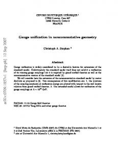
Fig. 1: Feynman rules for Noncommutative U (1) in background field gauge. In the calculation of section 2, we use Feynman gauge, α = 1.
We can compute Γ[0, A] by summing one-particle irreducible Feynman diagrams with classical fields Aµ on external legs and quantum fields Qµ appearing only in internal lines. The Feynman rules for conventional non-Abelian gauge theory in the background field gauge are given in [34]. The Feynman rules for the noncommutative U (1) theory can be obtained from [34] by simply replacing the structure constants fabc by sin( 21 pµ θ µν kν ), where p, k are the momenta of two of the gluons entering the vertex. The Feynman rules relevant for the calculations of this paper are shown in fig. 1. 4
The explicit gauge invariance of Γ[0, A] simplifies computations in the gauge theory. The bare field strength, when expressed in terms of the renormalized coupling and gauge field, is 1/2
1/2
bare Fµν = ZA (∂µ Aν − ∂ν Aµ − igZg ZA [Aµ , Aν ]),
(2.10)
where the Zg , ZA are the coupling constant and field renormalizations 1/2
g bare = Zg g, Abare = ZA Abare . µ µ −1/2
Gauge invariance of (2.10) implies that ZA
(2.11)
= Zg . This means that the β-function can
be computed from ZA , which only requires knowledge of the two-point function of the theory. The background field gauge is also very useful for comparing field theory amplitudes with the zero slope limit of string theory amplitudes. Ref. [35] derived the β-function of Yang-Mills theory by calculating the effective action of strings in a background magnetic field. Ref. [36] pointed out a correspondence between loop amplitudes in the background field gauge and loops calculated using string motivated rules.
More recently, [37][38][39]
calculated two, three and four point gauge boson amplitudes in open bosonic string theory. Using a suitable prescription for continuing the amplitudes off-shell, the renormalization constants obtained from the zero slope limit of the string theory amplitudes were observed to respect the background field gauge Ward identities. We will see below that the low energy limit of the string theory amplitudes in our D-brane construction reproduce the field theory loop amplitudes calculated in the background field gauge. In fig. 2 we show the one loop diagrams for the two-point function in U(1) noncommutative gauge theory. In ordinary gauge theory the tadpole diagrams give vanishing contributions because
Z
dd p =0 p2
(2.12)
in dimensional regularization. However, in the noncommutative theory these graphs are nonvanishing and must be included to obtain a gauge invariant answer. The sum of the diagrams of Fig. 1 is Πµν =2g
2
Z
�� � � dd q ˜q 8(p2 Gµν − pµ pν ) 2Gµν (p + 2q)µ (p + 2q)ν 2 p , sin ( ) + (d − 2) − 2 (2π)d 2 q 2 (p + q)2 q 2 (p + q)2 q (2.13)
where p˜µ = θ µν pν . Using the identity sin2 (x) = 12 (1 − cos(2x)) the field theory expression
separates into two parts, one independent of θ and one with a cos(˜ pq) in the integrand. The 5
�� A ��
�� �� A A �� ��
�� A ��
�� A ��
�� �� A A ����
�� A ��
Fig. 2: One loop contributions to the two-point function.
term independent of θ corresponds to the planar diagrams [10], and gives an expression identical to ordinary Yang-Mills theory with the usual group theory factor facd fbcd = N δab replaced by 2. This piece is divergent in four dimensions and gives a 1/ǫ pole. From this term one can extract the β-function of the noncommutative theory [21][14][13]. The term with the cos(˜ pq) corresponds to the nonplanar graphs and is ultraviolet finite. To compare with the string theory calculation in section 3 it is best to combine the propagators using Feynman parameters and then do the momentum integral via the method of Schwinger parameters. The contribution of the planar graphs is ΠP µν
ig 2 µ4−d 2 (p Gµν −pµ pν ) = (4π)d/2
Z
0
∞
dt
Z
1
2
dx t1−d/2 e−p
tx(1−x)
(8−(d−2)(1−2x)2 ). (2.14)
0
The contribution from the nonplanar graphs is ΠNP µν =
ig 2 − (4π)2
Z
0
Z dt
∞
1
dx t
�
−1 −p2 tx(1−x)−˜ p2 /4t
e
0
� 2 (p Gµν− pµ pν )(8 − 2(1 − 2x) ) − 2 p˜µ p˜ν t (2.15) 2
2
where since these diagrams are finite we have set d = 4. The planar diagrams are ultraviolet divergent and to regulate this divergence we take 6
d = 4 − 2ǫ. The result of evaluating the integral in (2.14) is ΠP µν
�� � �−ǫ i2g 2 2 −p2 Γ[ǫ]Γ[1 − ǫ]2 11 − 7ǫ = (p G − p p ) µν µ ν (4π)2 3 − 2ǫ 4πµ2 Γ[2 − 2ǫ] � � � � 1 −p2 ig 2 22 2 (p Gµν − pµ pν ) − ln + ... , = (4π)2 3 ǫ µ2
(2.16)
where ... is a constant. The nonplanar diagrams evaluate to ΠNP µν
Z 1 h p ig 2 2 2 =− dx 2(p G − p p )(8 − 2(1 − 2x) )K (p˜ p x(1 − x)) µν µ ν 0 (4π)2 0 � p p˜µ p˜ν 2 2 , p x(1 − x)) −16 4 p p˜ x(1 − x)K2 (p˜ p˜ � � � � � ig 2 22 p˜µ p˜ν 2 2 2 =− (p Gµν − pµ pν ) − ln p p˜ + ... − 32 4 + ... (4π)2 3 p˜
(2.17)
where we have expanded in p2 p˜2 to lowest order and kept the most infrared singular terms. The nonplanar graphs give rise to ln(p2 p˜2 ), as first observed in [26], as well as the correction to the photon polarization tensor of the form p˜µ p˜ν /˜ p4 , observed in [28][30]. This last term is interesting since it modifies the photon dispersion relation. We will see in the next section that the zero slope limit of the one loop string theory amplitude exactly reproduces the field theory answer (2.14)(2.15). The Schwinger parameter t in the field theory calculation is proportional to the modulus of the string world sheet while the Feynman parameter x is related to the separation of the vertex operators on the worldsheet.
3. The String Theory Calculation In this section we reproduce the field theory results of section 2 using string theory. We will find a simple realization of the noncommutative U(1) gauge theory using D3-branes in bosonic string theory and perform a one loop string calculation which will yield, in the massless open string boundary of moduli space, the results of the previous section. A four dimensional pure U(1) gauge theory can be realized by taking the low energy limit of the theory on a single D3-brane of bosonic string theory stuck at an R22 /Z2 orbifold singularity. This can be accomplished [31][32] by choosing the action of the orbifold group on the Chan-Paton factors to be represented by either of the two one-dimensional 7
representations of Z2 . The projection equation projects out the transverse scalars and we are left with only a gauge field. The noncommutative version of the pure U(1) gauge theory can be obtained by applying a constant magnetic field along the D-brane worldvolume. The quantum effective action of this gauge theory is encoded in the string theory effective action. An appropriate truncation of a string loop diagram should provide, in the low energy limit, the field theory answer. We will explicitly verify at the one loop level that the planar and non-planar two-point amplitudes for the photon on the cylinder in a background magnetic field reproduce the corresponding computations in the noncommutative gauge theory in the background field gauge. The correlation function of the photon field vertex operators on the disk shows that the low energy classical action on the brane is a noncommutative gauge theory with the usual replacement of conventional products by ⋆-products [9]. Comparison between the string theory calculation and the field theory fixes the normalization of the photon vertex operator to be V (z, k) = ig
Z
∂Σ
ds e · ∂s Xeik·X ,
(3.1)
where g is the tree level Yang-Mills coupling constant, eµ is the polarization of the photon, s is the coordinate on the worldsheet boundary ∂Σ and indices are contracted with the Gµν metric. The worldsheet topology of the one-loop diagram is a cylinder, which we represent in the complex z-plane as a rectangle of width π and height 2πit – where 0 ≤ t ≤ ∞ is the modulus of the cylinder – and with the edges y = 0 and y = 2πit identified: z = x + iy
0≤x≤π
y ≃ y + 2πt
0 ≤ y ≤ 2πt.
(3.2)
Open string vertex operators must be inserted on the boundaries of the cylinder at either x = 0 or x = π, with the positions given by w = iy and w = π + iy respectively. The full two-point function is obtained by summing over the planar (two vertex operators on the same boundary) and non-planar (each vertex operator on a different boundary) diagrams. These diagrams are given by A=
Z
0
∞
dt 2t
Z
0
2πt
dy1
Z
0
2πt
dy2 Z(t) < V (y1 , k1 )V (y2 , k2 ) >≡ eµ1 eν2 Πµν ,
(3.3)
where one should keep in mind when computing < . . . > if the diagram is planar or nonplanar. The different terms in (3.3) are easily understood. The 1/2t factor arises from 8
explicitly gauge fixing the path integral and dividing by the conformal Killing volume of the cylinder (which allows all vertex operators to be unfixed). Z(t) is the open string partition function of the vacuum under consideration, which in our case is that of an open string ending on D3-brane of bosonic string theory stuck at an orbifold singularity and in a background magnetic field. The correlator < . . . > is computed by contracting the fields using the Green’s function on the cylinder with boundary conditions modified by the background magnetic field. The open string partition function is a key ingredient in the measure of the correlation function (3.3). Worldsheet consistency conditions require projecting the open string spectrum onto states invariant under the action of the orbifold group. For our Z2 orbifold this is reflected in the partition function Z(t) = Tr(
1 + g −2tHo e ) = Z1 (t) + Zg (t), 2
(3.4)
where Ho is the open string Hamiltonian and g is the Z2 generator. The Z2 action on the endpoints of the string corresponding to a stuck D3-brane just multiplies (3.4) by unity [31][32][40]. It is straightforward to show that p+1 Vp+1 (8π 2 α′ t)− 2 η(it)−24 2 p+1 p−25 27−3p 25−p Vp+1 (8π 2 α′ t)− 2 ϑ2 (0, it) 2 η(it) 2 , Zg (t) = idet(g + 2πα′ F )2 2 2
Z1 (t) = idet(g + 2πα′ F )
(3.5)
where we have left explicit the dimensionality of the brane (which will turn out to be useful when comparing to the field theory results from section 2). Fµν are the components of the background magnetic field. In order to compute the correlation function (3.3) we must solve for the Green’s function of the worldsheet scalars on the cylinder. The background magnetic field along the brane does not modify the equations of motion of the open strings ending on it, but it does change the boundary conditions on the worldsheet fields. Worldsheet coordinates along the brane satisfy the following boundary conditions2 : gµν ∂n X + 2πiα Fµν ∂s X ν
′
ν
∂Σ
= 0.
(3.6)
Here gµν is the closed string metric (the metric that appears in the string sigma model action). The operators ∂n and ∂s are derivatives normal and tangential to the worldsheet 2
The coordinates transverse to the brane are projected out by the orbifold quotient.
9
boundaries ∂Σ. The correlation function of vertex operators < . . . > on a given worldsheet is computed from the propagators of the worldsheet fields, which can be found by solving the worldsheet wave equation while taking into account the boundary conditions (3.6). On the cylinder, the wave equation to be solved is 2 1 ρσ ∂w ∂w¯ Gρσ (w, w′ ) = −2πδ 2 (w − w′ )g ρσ + g . ′ α 2πt
(3.7)
The last term, which is proportional to the inverse area of the cylinder, is included in order to satisfy Gauss’ law and is compatible with the boundary conditions (3.6). The propagator we are interested in should solve (3.7), satisfy (3.6) at both boundaries of the cylinder, and respect the identification y ≃ y + 2πt of the cylinder. The solution is given
by
"
w − w′ i w+w ¯ ′ i log ϑ1 ( G (w, w ) ≡< X (w)X (w ) >= −α g | ) − log ϑ1 ( | ) 2πit t 2πit t !# 2 w+w ¯′ i ′ µν | ) ϑ ( w + w ¯ θ i Re2 (w + w ¯ ′ ) + Re2 (w − w′ ) � 1 2πit t + Gµν log ϑ1 ( | ) + log − ∗ w+ − , w ¯′ i 4πt 2πit t 2πα′ ϑ1 ( 2πit |t) (3.8) µν
′
µ
ν
′
′
µν
�
where w and w′ are points on the cylinder.
The propagator on the cylinder has a similar structure to the propagator on the disk. Here Gµν is the open string metric (the metric that defines the dispersion relation for open string fields), and θ µν is the noncommutativity parameter which appears in the definition of the ⋆-product. They are defined by � �µν 1 1 µν G = g g + 2πα′ F g − 2πα′ F �µν � 1 1 µν ′ 2 . F θ = −(2πα ) g + 2πα′ F g − 2πα′ F
(3.9)
The noncommutative field theory is obtained by taking the limit α′ ∼ ǫ → 0 and g ∼
ǫ1/2 → 0 , with the magnetic field kept constant [9].
For the two-point function of photon vertex operators we only need the propagator
for points on the boundaries. The correlator is given by = (∂w ∂w′ G µν + kρ kσ ∂w G µρ ∂w′ G σν ) ekρ kσ (G
ρσ
(w,w ′ )− 21 Grρσ (w,w)− 12 Grρσ (w ′ ,w ′ ))
= (−kρ kσ ∂w G ρσ ∂w′ G µν + kρ kσ ∂w G µρ ∂w′ G νσ ) ekρ kσ (G 10
ρσ
(w,w ′ )− 21 Grρσ (w,w)− 12 Grρσ (w ′ ,w ′ ))
(3.10)
where we have integrated the first term by parts. Grmn (w, w) is the renormalized prop-
agator, which regulates the divergences in the self-contractions by subtracting the short distance behaviour of the propagator. The proper renormalized propagator for open string vertex operators is given by Grρσ (w, w′ ) = G ρσ (w, w′ ) + α′ Gρσ (log |w − w′ |2 ),
(3.11)
where w and w′ are points on the same boundary. We will denote the combination in the exponent in (3.10) as 1 1 Geρσ (w, w′ ) ≡ G ρσ (w, w′ ) − Grρσ (w, w) − Grρσ (w′ , w′ ) 2 2
(3.12)
We will now consider in turn the results for the planar and non-planar diagrams. 3.1. Planar Two-point function Geρσ (w, w′ ) differs from G ρσ (w, w′ ) by a term that is independent of the position of the
vertex operators. On the x = 0 boundary it is given by3
ϑ ( i(y−y′ ) , it) 2 (y − y ′ )2 1 2π + i θ ρσ ǫ(y − y ′ ) Geρσ (w, w′ ) = −α′ Gρσ log 2π − ′ ϑ1 (0, it) 2πt 2
(3.13)
i ≡ −α′ Gρσ Γ(y − y ′ ) + θ ρσ ǫ(y − y ′ ), 2
where w = y, w′ = y ′ (or w = π + iy, w′ = π + iy ′ ), Gρσ is the open string metric and ǫ(x) is 1 for x > 0 and -1 for x < 0. On the x = π boundary the sign of the term proportional to θ ρσ changes sign4 . Note that we have used a ϑ-function identity to rewrite the propagator in a form conducive to taking the t → ∞ limit.
Plugging this expression into the correlator (3.10) we see that it has the familiar form
of the vacuum polarization diagram of the photon � ′ 2 < ∂s X µ eik·X (w1 )∂s X ν e−ik·X (w2 ) >= −α′2 k 2 Gµν − k µ k ν (∂y Γ)2 e−α k Γ ,
(3.14)
where k 2 = Gρσ kρ kσ and y = y1 − y2 . 3
Unlike Eq.(3.8) above, this expression is not manifestly periodic. However, it is straightfor-
ward to rewrite this expression in a form in which periodicity is manifest. 4
We thank H. Dorn for correspondence on this point.
11
Combining all the terms in (3.3) one is led to the following expression for the planar two-point function Z Z 2πt Z ∞ � ′ 2 dt 2πt P 2 dy1 dy2 Z(t) α′2 k 2 Gµν − kµ kν (∂y Γ)2 e−α k Γ , Πµν = −g 2t 0 0 0
(3.15)
where Z(t) is given by (3.5) and Γ by (3.13).
The task at hand is to identify in this string computation the noncommutative field theory result. We have to examine (3.15) in the decoupling limit specified in [9], which in particular requires taking the α′ → 0 limit. In this limit we only get contributions from corners of string moduli space. We will now show that we obtain the exact planar field
theory answer from the boundary of moduli space of the cylinder which is dominated by massless open strings5 , which comes from the t → ∞ limit. We therefore need the large t
expression of the integrand in (3.15). The large t expansions of Z(t) and of ∂y Γ are given
by Z(t) ≃ Vp+1 (8π 2 α′ t)−
p+1 2
e2πt + p − 1 + O(e−2πt ) � ∂y Γ ≃ 1 − 2x + 2 e−2πxt − e2πxt e−2πt ,
�
(3.16)
where x = y/2πt. Plugging these expressions into (3.15) and tossing out the contribution due to the tachyon, one gets (with d = p + 1 and g → gµ4−d ) Z 1 Z � −k2 tx(1−x) � ∞ g 2 µ4−d 2 P 1−d/2 2 Πµν = i dx t 8 − (d − 2)(1 − 2x) e , dt k G − k k µν µ ν (4π)d/2 0 0 (3.17) which is precisely the field theory answer (2.14). To obtain this result we rescaled t → t/α′
and y → y/α′ . In these new variables (with α′ → 0) any finite value of t is in the extreme
open string limit of the moduli space. In particular the excited open string corrections in ′
(3.16) become O(e−2πt/α ) which vanish in the decoupling limit. This will be discussed further in Section 4.
3.2. Non-Planar Two-point function The nonplanar propagator with w = π + iy and w′ = y ′ is given by " ϑ ( i(y−y′ ) , it) 2 ′ 2 π θ ρσ (y − y ′ ) (y − y ) 2 2π + + i − Geρσ = − α′ Gρσ log 2π ϑ′1 (0, it) 2t 2πt 2πα′ t # π . − g ρσ 2t 5
(3.18)
Note that since we are using bosonic string theory the field theory result is obtained only after removing by hand the divergence caused by the open string tachyon.
12
As in the planar diagram computation we expand (3.18) in the large t region. The asymptotics of the term proportional to the open string metric Gρσ is the same as for the planar diagram. The important differences are in the terms proportional to the closed string metric g µν and the noncommutativity parameter θ µν . The term proportional to θ µν does not contribute to the exponential in (3.10), but it plays a very important role in the derivative terms. Since this is a non-planar diagram for an oriented string, there is an overall factor of −1 since the ends of the string carry opposite charges. The final answer is given by Z Z 1 2 g 2 µ4−d ∞ ˜2 dt dx t1−d/2 e−k tx(1−x)−k /4t −i d/2 (4π) 0 0 � � � � 2 ˜ν . × k 2 Gµν − kµ kν 8 − (d − 2)(1 − 2x)2 − 2 k˜µ k t
ΠNP µν =
(3.19)
This expression is identical to that obtained from the nonplanar field theory graphs (2.15).
4. Discussion In the previous sections we have seen how the annulus (cylinder) amplitude of string theory in a background F field reproduces, in the decoupling limit of [9], the planar and nonplanar results of noncommutative gauge theory. Let us discuss this in more detail. Schematically the two-point function on the annulus is given in the open string channel by A∼
Z
∞
dt t 0
X
exp (−∆I t).
(4.1)
I
The index I labels all open string states and ∆I , basically the L0 eigenvalue, is the mass squared of state I plus momentum dependence. In the decoupling limit of [9] α′ → 0 and hence the string mass scale is sent to infinity. The oscillator contribution to ∆I is unaffected
by F and hence is just NI /α′ where NI is the total oscillator occupation number. So in the α′ → 0 limit all the excited open string states become much heavier than the massless one
and hence should decouple from the dynamics. The vanishing of the exponential corrections
in (3.17) and (3.19) illustrates this. This is similar to other decoupling limits such as those which show that field theories arise from branes separated by short distances. As pointed out in [26] and further discussed in [27][30]there are peculiar singularities indicating IR/UV mixing in the nonplanar noncommutative gauge theory results. These results have been interpreted to mean [26][27] that some closed string residue remains in the field theory, even 13
in the decoupling limit. So it is important to examine if and how decoupling is breaking down here. Generally, the only way decoupling can fail is for the interactions of the decoupled theory to have bad high energy behavior. If loops of massless open string states are UV divergent, then massive open string states will generally be excited, violating decoupling. If the decoupled field theory is divergent but renormalizable then there will be a mild violation of decoupling, but all the effects of the massive string states can be absorbed in a few “renormalized” couplings. For instance, g 2 ln(−p2 /µ2 ) in (2.16) becomes, in string theory, g 2 (ln(−p2 α′ ) + O(1)).
Now let us examine decoupling in the nonplanar diagrams that display mysterious
UV/IR singularities. We can write a caricature of the string amplitude (3.19) by suppressing the x integral, all numerical factors, and adding back in the effect of the first excited open string state. ANP ∼
Z
dt t1−d/2 e−k
2
˜ 2 /4t t−k
′
(1 + e−2πt/α + . . .).
(4.2)
˜ 2 /4t term in the exponential renders the UV region of the modular inteNote that the k gration (t → 0) completely finite for any nonzero k˜2 . This term is present in the field
theoretic amplitude (2.15) and represents the effect of the rapidly oscillating phases in the noncommutative gauge theory interaction vertices. These phases are enough to render the ˜2 . nonplanar amplitude finite for any nonzero k ˜ 2 . The contribution of the The smallest important value of t in (4.2) is roughly t ∼ k ˜2
′
first excited state is then ∼ e−2π k /α . In the decoupling limit α′ → 0 and this contribution vanishes for any nonzero k˜2 . The decoupled field theory amplitude is UV finite so decoupling cannot fail.
To further investigate this question let us keep α′ finite. There are then two regimes to consider. If k˜2 ≫ α′ then the excited open string state contribution is negligible and the decoupled field theory result is accurate. If k˜2 ≪ α′ , however, the small t region of the integral may be important. This depends on whether the field theory graph without
phase factors is UV divergent. It will be, for instance, if the space-time dimension d is large enough. If there is a small t UV divergence then all the excited open string states will become important. In this case the correct way to analyze the situation is to use channel duality and rewrite the amplitude in terms of closed string states. At small t only the lightest closed string states will contribute, giving a massless propagator 1/k 2 (assuming we drop the closed string tachyon). 14
The region where the closed string description is valid becomes smaller and smaller as we approach the decoupling limit α′ → 0. In this limit the region of validity shrinks to a set of measure zero. For all finite k˜2 the decoupled field theory describing only the lightest open string mode is exact. So the complete structure of the mysterious IR/UV singularities is contained in the open string description. Of course one can formally represent the behavior of the lightest open string in the dual closed string channel. But this requires a sum over closed string states of arbitrarily high mass and does not seem very transparent. This is the usual situation in dualities. A regime that has a simple description in one set of variables typically has a complicated description in the dual variables. To illustrate this point consider (4.2) for general d. The log divergence in d = 4 becomes a 1/k˜d−4 divergence. The massless closed strings will produce a 1/k 2 behavior for any d. To produce the open string behavior will require a sum over all the closed string states. There is at least one situation where decoupled field theory results can be reproduced from the lightest closed string state6 . This is the case where a nonrenormalization theorem exists [41][42][43]. The contribution of excited open string states vanishes, typically because they are in long multiplets of an extended supersymmetry algebra. The exact amplitude is given by the lightest open string state, and so this must also agree with the closed string answer. This mechanism seems to require lots of supersymmetry, and usually applies only to special amplitudes. So it seems questionable whether it will be helpful in giving a general explanation for these mysterious singularities. Note Added In the past week the papers [44][45][46] appeared on the archive. They overlap substantially with ours. Acknowledgments We would like to thank Allan Adams, Sergei Gukov, John McGreevy, Hirosi Ooguri, Maxim Perelstein, John Schwarz, Lenny Susskind, Nick Toumbas and Edward Witten for discussions. We would like to thank Iain Stewart for help making the figures. J.G. and T.M. are supported in part by the DOE under grant no. DE-FG03-92-ER 40701. M.R. is supported by the Caltech Discovery Fund under grant no. RFBR 98-02-16575 and DEFG-05-ER 40219. M.K. is supported by an NSF graduate fellowship. S.S. is partially supported by NSF grant 9870115. 6
This observation is due to Lenny Susskind.
15
References [1] A. Connes, M.R. Douglas and A. Schwarz, “Noncommutative Geometry and Matrix Theory: Compactification on Tori”, JHEP 9802(1998) 003, hep-th/9711162. [2] M.R. Douglas and C. Hull, ”D-branes and the Noncommutative Torus”, JHEP 9802 (1998) 008, hep-th/9711165. [3] B. de Wit, J. Hoppe and H. Nicolai, ”On The Quantum Mechanics of Supermembranes,” Nucl. Phys. B305 (1988) 545. [4] Y.-K. E. Cheung and M. Krogh, ”Noncommutative Geometry From 0-Branes In A Background B Field,” Nucl. Phys. B528 (1998) 185, hep-th/9803031 [5] C.-S. Chu and P.-M. Ho, ”Noncommutative Open String And D-Brane,” Nucl. Phys. 550(1999)151, hep-th/9812219; ”Constrained Quantization of Open String In Back¯ ground B Field and Noncommutative D-brane,” hep-th/9906192. [6] V. Schomerus, ”D-Branes And Deformation Quantization,” JHEP 9906:030 (1999), hep-th/9903205. [7] F. Ardalan, H. Arafei and M. M. Sheikh-Jabbari, ”Mixed Branes and M(atrix) Theory on Noncommutative Torus,” hep-th/980367; ”Noncommutative Geometry From Strings and Branes,” JHEP 02 016 (1999) hep-th/9810072; ”Dirac Quantization of Open Strings and Noncommutativity in Branes,” hep-th/9906161. [8] D. Bigatti and L. Susskind, hep-th/9908056 . [9] N. Seiberg and E. Witten, “ String Theory and Noncommutative Geometry”, JHEP 9909 (1999) 032, hep-th/9908142. [10] T. Filk, ”Divergences in a Field Theory on Quantum Space”, Phys. Lett. B376 53. [11] J.C. Varilly and J.M. Gracia-Bondia, ”On the ultraviolet behaviour of quantum fields over noncommutative manifolds”, Int. J. Mod. Phys. A14 (1999) 1305, hepth/9804001. [12] M. Chaichian, A. Demichev and P. Presnajder, “Quantum Field Theory on Noncommutative Space-times and the Persistence of Ultraviolet Divergences”, hepth/9812180; “Quantum Field Theory on the Noncommutative Plane with E(q)(2) Symmetry”, hep-th/9904132. [13] C.P.Martin, D. Sanchez-Ruiz, “The One-loop UV Divergent Structure of U(1) YangMills Theory on Noncommutative R4 ”, Phys. Rev. Lett. 83 (1999) 476-479,hepth/9903077 [14] M. Sheikh-Jabbari, “Super Yang-Mills Theory on Noncommutative Torus from Open String Interactions”, Phys. Lett. B450 (1999) 119, hep-th/9810179; “One Loop Renormalizability of Supersymmetric Yang-Mills Theories on Noncommutative Torus”, JHEP 06 (1999) 015, hep-th/9903107; “On the Deformation of Λ-Symmetry in B-field Background”, Phys. Lett. B477 (2000) 325, hep-th/9910258; ”Noncommutative Super Yang-Mills Theories with 8 Supercharges and Brane Configurations”, hep-th/0001089. 16
[15] H. Grosse, T. Krajewski and R. Wulkenhaar, ”Perturbative quantum gauge fields on the noncommutative torus”, hep-th/9903187. [16] S. Cho, R. Hinterding, J. Madore and H. Steinacker, “Finite Field Theory on Noncommutative Geometries”, hep-th/9903239. [17] E. Hawkins, “Noncommutative Regularization for Practical Man”, hep-th/9908052. [18] I. Chepelev and R. Roiban, “Renormalization of Quantum Field Theories on Noncommutative Rd , I. Scalars,” hep-th/9911098. [19] G. Arcioni and M. A. Vazquez-Mozo, “Thermal effects in perturbative noncommutative gauge theories”, JHEP 0001 (2000) 028, hep-th/9912140. [20] S. Iso, H. Kawai and Y. Kitazawa, “Bi-local fields in noncommutative field theory”, hep-th/0001027. [21] H. Grosse, T. Krajewski and R. Wulkenhaar, ”Renormalization of noncommutative Yang-Mills theories: A simple example”, hep-th/0001182. [22] I.Ya. Aref´eva, D.M. Belov and A.S. Koshelev, ”Two-Loop Diagrams in Noncommutative φ44 theory”, hep-th/9912075; ”A Note on UV/IR for Noncommutative Complex Scalar Field”, hep-th/0001215. [23] I.Ya. Aref´eva, D.M. Belov, A.S. Koshelev and O.A. Rytchkov, ”UV/IR Mixing for Noncommutative Complex Scalar Field Theory, II (Interaction with Gauge Fields)”, hep-th/0003176. [24] F. Ardalan and N. Sadooghi, ”Axial Anomaly in Non-Commutative QED on R4 ”, hep-th/0002143. [25] J.M. Gracia-Bondia and C.P. Martin, ”Chiral Gauge Anomalies on Noncommutative R4 ”, hep-th/0002171. [26] S. Minwalla, M.V. Raamsdonk and N. Seiberg, “Noncommutative Perturbative Dynamics”, hep-th/9912072. [27] M.V. Raamsdonk and N. Seiberg, “ Comments on Noncommutative Perturbative Dynamics”, hep-th/0002186. [28] M. Hayakawa,“Perturbative analysis on infrared and ultraviolet aspects of noncommutative QED on R4 ,” hep-th/9912167. [29] W. Fischler, E. Gorbatov, A. Kashani-Poor, S. Paban, P. Pouliot and J. Gomis, “Evidence for winding states in noncommutative quantum field theory,” hep-th/0002067. [30] A. Matusis, L. Susskind and N. Toumbas, “The IR/UV connection in the noncommutative gauge theories,” hep-th/0002075. [31] M.R. Douglas, ”Enhanced Gauge Symmetry in M(atrix) Theory”, JHEP 9707 (1997) 004, hep-th/9612126. [32] D.E. Diaconescu, M.R. Douglas and J. Gomis, ”Fractional Branes and Wrapped Branes”, JHEP 9802 (1998) 013, hep-th/9712230. [33] B.S. DeWitt, Phys. Rev. 162 (1967) 1195, 1239; in Dynamic Theory of Groups and Fields (Gordon and Breach, 1965) 17
[34] L. F. Abbot, Nucl. Phys. B185 (1981) 189-203. [35] R.R. Metsaev and A.A. Tseytlin, “One Loop Corrections to String Theory Effective Actions”, Nucl. Phys. B298 109 (1988). [36] Z. Bern and D. C. Dunbar, Nucl. Phys. B379(1992) 567-601. [37] P. Di Vecchia, A. Lerda, L. Magnea, R. Marotta and R. Russo, “String techniques for the calculation of renormalization constants in field theory”, Nucl.Phys. B469 (1996) 235, hep-th/9601143. [38] P. Di Vecchia, A. Lerda, L. Magnea, R. Marotta, “Gauge theory renormalizations from the open bosonic string”, Phys. Lett. B351 (1995) 445, hep-th/9502156. [39] E. Alvarez and C. G´omez, “Ultraviolet and Infrared freedom from string amplitudes”, JHEP 9910 (1999) 018, hep-th/9907205. [40] D.E. Diaconescu and J. Gomis, “Fractional Branes and Boundary States in Orbifold Theories”, hep-th/9906242. [41] M.R. Douglas and M. Li, ”D-Brane Realization Of N=2 Superyang-Mills Theory In Four-Dimensions,” hep-th/9604041. [42] M.R. Douglas, D. Kabat, P. Pouliot and S. H. Shenker, ”D-Branes And Short Distances In String Theory,” Nucl. Phys. B485 85 (1997). [43] C. Bachas and E. Kiritsis, ”F(4) Terms In N=4 String Vacua,” Nucl. Phys. Proc.Suppl. 55B 194(1997). [44] O. Andreev and H. Dorn, ”Diagrams of Noncommutative Φ3 Theory from String Theory”, hep-th/0003113. [45] Y. Kiem and S. Lee, “UV/IR Mixing in Noncommutative Field Theory via Open String Loops”, hep-th/0003145. [46] A. Bilal, C.-S. Chu and R. Russo, “ String Theory and Noncommutative Field Theories at One Loop”, hep-th/0003180. [47] A. Abouelsaood, C.G. Callan, C.R. Nappi and S.A. Yost, ”Open Strings in Background Gauge Fields”, Nucl. Phys. B280 (1987) 599-624.
18