Nonidentical circle packing problem: multiple disks installed in a rotating circular container W. A. Oliveiraa∗, L. L. Salles Netob , A. C. Morettic and E. F. Reisa a Department b Department
of Mathematics, Federal Technological University of Paran´a, PR, Ponta Grossa, Brazil
of Science and Technology, Federal University of S˜ao Paulo, S˜ao Jos´e dos Campos, SP, Brazil c School
of Applied Science, University of Campinas, Limeira, SP, Brazil
E-mail:
[email protected] [Oliveira];
[email protected] [Salles Neto];
[email protected] [Moretti];
[email protected] [Reis]
Abstract In this work we propose a heuristic algorithm for the layout optimization for disks installed in a rotating circular container. This is a unequal circle packing problem with additional balance constraints. It proved to be an NP-hard problem, which justifies heuristic methods for its resolution. The main feature of our heuristic is based on the selection of the next circle to be placed inside the container according to the position of the system’s center of mass. Our approach has been tested on a series of instances up to 55 circles and compared with the literature. Computational results show good performance in terms of solution quality and computational time for the proposed algorithm. Keywords: Layout problem, Nonidentical circle packing, Heuristic.
1
Introduction
We study how to install unequal disks in a rotating circular container [8], which is an adaptation of the model for the two-dimensional (2D) unequal circle packing problem with balance behavioural constraints. This problem arises in some engineering applications: development of satellites and rockets, multiple spindle box, rotating structure and so on. The low cost and high performance of the equipment requires the best internal configuration among different geometric devices. This problem is known as layout optimization problem (LOP), and consists in placing a set of circles in a circular container of minimum envelopment radius without overlap and with minimum imbalance. Each circle is characterized by its radius and mass. There, the original three-dimensional (3D) case (the equipment must rotate around its own axis) is simplified: different two-dimensional circles (see, Figure 1(c)) represent three-dimensional cylindrical objects to be placed inside the circular container. ∗ Corresponding
author
1
Figure 1 illustrates the physical problem. Item (a) shows a rotating cylindrical container. The symbol ω and the arrow illustrates the rotation around the axis of the equipment, ω is the angular velocity. In another viewpoint, item (b) shows the interior of the equipment where distinct circular devices need to be placed. In this example, six cylinders are placed, in which the radii, masses and heights are not necessarily equal. Research on packing circles into a circular container has been documented and used to obtain good solutions. Most of them uses heuristic, metaheuristic and hybrid methods. There are only a few publications discussing the disk problems with balance constraints. This problem was proposed by Teng et al. [8], where is described a series of intuitive algorithms combining the method of constructing the initial objects topo-models with the model-changing iteration method, and numerical tests on two instances of the problem were made. LOP is a combinatorial problem surprisingly difficult and has been reported to be NP-hard [3, 9]. Fei and Teng [2] presented a modified genetic algorithm called decimal coded adaptive genetic algorithm to solve the LOP. Yi-Chun Xu et al. [11] developed a version of genetic algorithm called order-based positioning technique, which orders the inclusion of the circles to be placed in the container. Qian et al. [7] extended the work [2] by introducing a genetic algorithm based on human-computer intervention, in which a human expert examines the locally optimal solution that can be obtained through the loops of many generations and designs new solutions. Methods based on particle swarm optimization (PSO) have been frequently used to solve this problem. Ning et al. [6] developed a PSO method based-mutation operator. This approach can escape from the local minima, maintaining the characteristic of fast speed of convergence. Zhou et al. [12] proposed a hybrid approach based on constraint handling strategy suit for PSO, where improvement is made by using direct search to increase the local search ability of the algorithm. Xiao et al. [10] presented two nature-inspired approaches based on gradient search, the first hybrid with simulated annealing (SA) method and the second hybrid with PSO method. Lei [5] presented an adaptive PSO with a better search performance, which employs multi-adaptive strategies to plan large-scale space global search and refined local search to obtain global optimum. In this paper, we propose a new heuristic to solve the LOP. The basic idea of our approach, called center-of-mass-based placing technique (CMPT), is to place each circle according to the current position of the center of mass of the system. The best results for a selected set of instances are found in [5, 6, 10, 12]. To validate our approach, we compare the results of our heuristic with these instances. Computational results show good performance in terms of solution quality and computational time. The paper is organized as follows. In Section 2, we present a formal definition of the unequal circle packing problem with balance constraints, and some definitions are established. In Section 3, we describe our heuristic. In Section 4, we present and analyze the experimental results, and in Section 5, we conclude the paper.
2
Problem formulation
We consider the following layout optimization for the disks installed in a rotating circular container: given a set of circles (not necessarily equal), find the minimal radius of a circular container so that all circles can be packed into the container without overlap, and the dynamic equilibrium of the system 2
ω (a)
6
r3
3
5
1
�
(c)
2 r
7
(b)
4
Figure 1: Circular devices inside a rotating circular container and a feasible solution should be minimized. The associated decision problem is stated as follows. Consider a circular container of radius r, a set of n circles i of radii ri and mass mi , i ∈ N = {1, . . . , n}. There may be several circles with the same radius or mass. Let (x, y)T be the coorT the center coordinates of the circle i. Let f (z) = r dinates of the container center, and (xi , yi )� 1 � �2 � �2 n n be the first objective function, and f2 (z) = ∑ mi ω2 (xi − x) + ∑ mi ω2 (yi − y) the second i=1
i=1
objective function, which measures the shift in the dynamic equilibrium of the system caused by the rotation of the container. We can consider ω = 1, since this does not affect the optimality of f2 . The problem is to determine if there exist 2n + 3 real numbers stored in the vector of variables z = (r, x, y, x1 , y1 , x2 , y2 , . . . , xn , yn )T that satisfies the following mathematical formulation. (LOP)
Minimize f (z) = λ f1 (z) + β f2 (z) subject to � � � 2 2 r � max ri + (xi − x) + (yi − y) ,
1�i�n (xi − x j )2 + (yi − y j )2 2n+3
z∈R
� (ri + r j )2 , i �= j ∈ N,
(1) (2)
, λ, β ∈ (0, 1).
Constraint (1) states that circle i placed inside the container should not extend outside the container, while constraints (2) require that the circles placed inside the container cannot overlap. Note that any pair of coordinates (x, y) or (xi , yi ) can be chosen and fixed. Figure 1(c) illustrates a typical feasible solution to the LOP. The circles are numbered from 1 to 7, r3 is the radius of the circle 3, there is no overlap between the circles and the seven circles are completely placed into the larger circle of radius r (radius of the container).
2.1
Definitions
We develop a constructive heuristic guided by a simple strategy. A suboptimal solution is reached after gradually placing a circle at a time inside the container. Each circle is placed in an Euclidean coordinates system on the following evaluation criteria: select as the new position of the circle according to the current center of mass of the system; it cannot overlap with the circles placed earlier; one 3
attempts to fill the wasted spaces after placing this circle; and in the end, select as the new coordinates of the container center that completely eliminates the dynamic imbalance of the system. To perform the above criteria we need some notations and definitions.�We denote by X(i) = (xi , yi )T the center coordinates of the circle i, by d(i, j) = d(X(i), X( j)) = (xi − x j )2 + (yi − y j )2 the Euclidean distance between the center coordinates of the circles i and j, and by Γ(i, j) = {(1 − λ)X(i) + λX( j) : 0 � λ � 1} the set of points on the line segment whose endpoints are X(i) and X( j). Figure 3(a) illustrates the set Γ(5, 10). Definition 1 (Contact Pair) If d(i, j) = ri + r j , we say that {i, j} is a Contact Pair of circles. Definition 2 (Layout) A partial Layout, denoted by L, is a partial pattern (layout) formed by a subset of the m � 2 coordinates of the circle centers, which have already been placed inside the container without overlap, and m − n circles that remain to be placed into the container. Assume in addition that the container itself is in L. If m = n, then L is a complete solution. Figure 2(b) illustrates a partial Layout formed by 16 circles placed inside the container. Among others, {10, 5} and {8, 15} are Contact Pairs. Definition 3 (Placed Cyclic Order) Let C = i1 i2 · · · it−1 it , i p ∈ N, p = 1, . . . ,t, be a cyclic order of circles, which have already been placed inside the container without overlap. In addition, the intersection of any two sets Γ(i p , iq ), where i p , iq are in C, have only one of its endpoints in common. We say that C is a Placed Cyclic Order. Definition 4 (Contact Cyclic Order) Let C be a Placed Cyclic Order. If the circles are two by two Contact Pairs in C, we say that C is a Contact Cyclic Order. Given a C = i1 i2 · · · i p−1 i p i p+1 · · · it−1 it , we say that the circles i1 , i2 , · · · , i p−1 are in counterclockwise order in relation to circle i p and the circles i p+1 , · · · , it−1 it are in clockwise order in relation to circle i p . Definition 5 (Main Area) Let C be a Placed Cyclic Order. We say that the area bounded by the union of the line segments Γ(i p , iq ), where i p , iq are in C, is the Main Area of C, which is denoted by A(C). Figure 2(a) illustrates a Contact Cyclic Order C¯ formed by 12 circles placed inside the container. ¯ it is illustrated a Note that all {i, j} in C¯ are two by two Contact Pairs. In item (b), in addition to C, Contact Cyclic Order C formed by 4 circles. Note that all circles in C (dashed lines) are completely ¯ This is a feature of our approach, since several Contact Cyclic Order are obtained placed on A(C). by circling each other. This approach is an important requirement, since it can yield a more compact layout. Let N¯ ⊂ N be a subset of circles placed inside the container. We denote the centroid of N¯ by the 1 coordinates XC = |N| ¯ ∑ X(i). i∈N¯
Definition 6 (Border) Let L be a partial Layout and C be a Contact Cyclic Order. If the center of each circle in L belongs to A(C), we say in addition that C is the Border of the partial Layout L.
4
L
12 •
12 •
6• 10 •
11 •
6•
15 •
10 •
11 •
15 •
4• 5•
•
2•
8
5• 1•
9•
•
•
XCM
•
•
16
3 9•
•
7
8
•
16
•
14
•
7
•
•
14
13 •
13
C = 5|9|13|7|14|16|8|15|11|6|12|10
C = 1|3|2|4 C = 5|9|13|7|14|16|8|15|11|6|12|10
(a)
(b)
Figure 2: Two Contact Cyclic Orders and a partial Layout
Figure 2(b) illustrates the Border C¯ (12 circles) of the partial Layout L (16 circles). Note that ¯ On the other hand, C = 1|3|2|4 is not a Border of L, since all circle centers in L belong to A(C). X(5) ∈ / A(C). We consider two cases of inclusion for placing circles. In the first case, we require that the circle k to be included must touch at least two previously placed circles. After this, in the second case, we require that another circle � to be included occupies the wasted spaces after placing the circle k. This is a reasonable requirement, since it will generally yield a more compact layout than one defined by separate circles. These two cases of inclusion can be explained by a partial Layout of the LOP example with seven existing circles illustrated in Figure 3. In item (a), it is shown the first case of inclusion. There are two positions to place the circle 9 (dashed lines) touching the Contact Pair {1, 7}, and two positions to place the circle 6 (dashed lines) touching the Contact Pair {2, 3}. Each position can be obtained by the solutions of the following particular case of the problems of Apolonio [1]. � (x − xi )2 + (y − yi )2 = rk + ri p p p � (3) (x − xi )2 + (y − yi )2 = rk + ri q q q
We denote by St(k, i p , iq ) the coordinates of the solution of the System (3) which does not belong to A(C). Note that the System (3) has two real solutions whenever d(i p , iq ) � ri p + riq + 2rk . In Figure 3(a), by choosing St(9, 7, 1) as the coordinates of the circle 9, we obtain a feasible layout. However, it is not enough to choose St(6, 2, 3) as the coordinates of the circle 6, because the circle 6 overlaps the circles 1 and 5. In our approach, we always select the coordinates St(k, i p , iq ) ∈ / A(C) in order to place the new circle k touching the Contact Pair {i p , iq } in the Border C (in Figure 3(a), we have k = 6 and {i p , iq } = {2, 3}), but due to the potentially large differences in the radii, it is possible to occur overlap with the circles in the Border C. As it is illustrated in Figure 3(a), we get around this situation by repositioning the circle k to the coordinates of the solution of new System (3) for k, i p¯ and iq¯ , where now the circle 5
k touches the circles i p¯ and iq¯ (in Figure 3(b), we have k = 6, i p¯ = 1 and iq¯ = 5). This first case of inclusion and the possible reposition defines the following placement approach. Definition 7 (External Placement) Let L be a partial Layout and C be the Border of L. An External Placement is the placement of a circle k inside the container, so that there is no overlap, its center does not belong to A(C), and it becomes Contact Pair with at least two circles in C. We denoted an External Placement by pE (k). The External Placement is always selected outside A(C), however if there is overlap on C, the repositioning of the new circle k (as explained above) is done in the following routine. Procedure 1: External Placement routine Input: a circle k, a Contact Pair {i p , iq }, a Partial Layout L and the Border C Output: an External Placement pE (k), p and q Step 1. Calculate St(k, i p , iq ) by System (3) and pE (k) ← St(k, i p , iq ). If the circle k does not overlap any circles in C stop, otherwise go to Step 2. Step 2. While there is overlap between the circle k and the circles in C repeat. If the circle k overlaps the circle i p¯ furthest with respect to the counterclockwise order of the Border C, p ← p, ¯ and if the ¯ and circle k overlaps the circle iq¯ furthest with respect to the clockwise order of the Border C, q ← q, choose pE (k) as the solution of the System (3) that is furthest from the centroid of the circles in L with respect to the Euclidean distance. First, if the new circle k does not overlap any circles in Border C, the External Placement routine selects pE (k) = St(k, i p , iq ). In our approach, this case is the most convenient way to place the next circle. However, if there is overlap, in Step 2 the routine identifies such circles (i p¯ and iq¯ ) in order to reposition the circle k further from the centroid of the Partial Layout, eventully avoiding any kind of overlap. To obtain a more compact layout, after including the circle k, it is checked the possibility of including another circle to occupy the wasted spaces after placing the circle k. We check among the remaining circles outside the container (preferably the largest one) if there is a circle � that can be placed into the container in a centralized position without overlap. Each centralized position is the centroid coordinates of a certain set of circles which includes the circle k and the two circles touching the circle k. Figure 3(b) illustrates the second case of inclusion, which we can investigate the possibility of positioning a circle in the wasted space after placing the circle 9 touching the Contact Pair {1, 7} (centroid XˆC of the circles {1, 7, 9}), and in the wasted space after placing the circle 6 touching the circles 1 and 5 (centroid X¯C of the circles {1, 2, 3, 4, 5, 6}). Definition 8 (Internal Placement) Let L be a partial Layout, C be the Border of L, and {i p , k}, {k, iq } be Contact Pairs in C, where k is the previous circle included. An Internal Placement is the placement of a circle � inside the container, so that its center belongs to A(C), � does not overlap with any other ¯ where {k, i p , iq } ⊆ N. ¯ circle, and the center of � is placed at the centroid coordinates of the subset N, 6
6•
6•
9•
Γ(5, 10) • 5 •
•
(a)
•
2
5• •
7• 9
10
6•
1
•
•
9•
4
� X C
•
6•
•
•
2
4
•
3
A(C) C = · · · |7|1|2|3|4|5|10| · · ·
10
XC
7•
•
3
•
1•
A(C) C = · · · |7|9|1|6|5|10| · · ·
(b)
Figure 3: Two cases of inclusion: (a) External Placement and (b) Internal Placement
¯ �), meaning that � is to be placed at the centroid coordiWe denote an Internal Placement by pI (N, ¯ nates XC of N. Let L be a partial Layout and C be the Border of L. In our algorithm, each positioning in the first case of inclusion is always done by looking at the Contact Pairs in the Border C. Suppose that the remaining circle k is selected to be placed touching the Contact Pair {i p , iq } in C. The placement of the circle k causes the addition of one element in L and one index in C, and perhaps the removal of some indices from C. This will be represented by the following operation. O+ − (k, i p , i p+s )(C) = C + {k} − {i p+1 , . . . , i p+s−1 } = i1 i2 · · · i p k i p+s · · · it−1 it , where 1 � s � �(t − 2)/2�. With this choice for s there are fewer indices between p and p + s than p + s and p. The operation O+ − (k, i p , i p+s )(C) applied to C means that the circle k was placed inside the container touching the circles i p and i p+s without overlap. Then the index k is added to C, the subset of indices {i p+1 , . . . , i p+s−1 } between p and p + s is removed from C, and the coordinates X(k) are added to the partial Layout L. Note that if s = 1 there is no removal of indices from C, and the index k is inserted in C between the indices i p and i p+1 . The possible placement of the circle � after the placement of the circle k only causes the possible addition of the coordinates X(�) to the partial Layout L. In our approach, we require the imbalance of the system be zero. It seems intuitive that this requirement may result in a good solution. However, this requirement � is easy to achieve.�We denote n
the center of mass of the system by XCM = (yCM , yCM ) = (1/ ∑ mi ) i=1
n
n
i=1
i=1
∑ mi xi , ∑ mi yi , then one
can shift the center of the rotating circular container to the center of mass of the system to have zero imbalance. This shift is made at each outer iteration and at the end of the algorithm. Thus, if the Layout L represents a complete solution of the LOP, we denote the radius r of the container by r = R(L) ≡ max {rik + d(XCM , X(ik ))}. Moreover, the index where R(L) is reached is denoted by 1�k�t
kmax ≡ arg(R(L)).
7
A postoptimization is performed after the algorithm builds a complete solution (represented by Layout L), which contemplates improvements via circle repositioning at the Border C of L. This postoptimization process causes changes in C, where an index is removed and then it is repositioned in C by operation O+ − . The removal of the index from C will be represented by the following operation. D(i p )(C) = i1 i2 · · · i p−1 i p+1 · · · it−1 it . The operation D(i p )(C) applied to C means that the circle i p is deleted from its position. We delete the current X(i p ) from the Layout L, and we test if a new position pE (i p ) for i p improves the radius R(L) of the container.
3
Center-of-mass-based placing technique (CMPT)
We present a new placing technique which yields compact layouts and quality solutions in an efficient manner. Let α = (α(1), α(2), . . . , α(n)) be a permutation of (1, 2, . . . , n). We place the circles in the partial Layout L one by one according to the order defined by this permutation and their radii. Given a order of inclusion, the first circles α(1), α(2), α(3) and α(4) must be positioned as follows. Procedure 2: Initial layout routine Input: the circles α(1), α(2), α(3) and α(4) Output: an initial Layout L and the initial Border C Place the circle α(1) at coordinates X(α(1)) = (0, 0). Choose an arbitrary angle θ, 0 � θ < 2π, and place the circle α(2) at coordinates X(α(2)) = ((rα(1) + rα(2) ) cos θ, (rα(1) + rα(2) ) sin θ). For each circle α(3) and α(4), solve the System (3) and place them at coordinates X(α(3)) = (xα(3) , yα(3) ) = St(α(2), α(1), α(2)) and X(α(4)) = St(α(4), α(1), α(2)) without overlap. L = {X(α(1)), X(α(2)), X(α(3)), X(α(4))} and C ← α(1)α(3)α(2)α(4). Figure 2(b) illustrates the initial L = {X(1), X(2), X(3), X(4)} and the initial Border C = 1|3|2|4. Suppose we have already placed the circles (α(1), α(2), . . . , α(k − 1)), we describe our approach for placing the circle α(k), and after that, we verify the possibility of placing another circle α(�), k < � � n. When we place the circle α(k) (where k > 4, see Procedure 2), we require that the circle touches at least two previously placed circles (see Figure 3(a) and Procedure 4). This will generally yield a more compact layout. However, we can increase the compactness of the layout if the wasted spaces after placing the circle α(k) can be occupied by another circle α(�) (see Figure3(b) and Procedure 4). We observe that for each additional circle, the envelopment radius of a layout is generally enlarged. In order to minimize the rate of growth of this radius during inclusions, we must properly choose a new position for circle α(k) which yields a smaller envelopment radius. Our strategy CMPT attempts to reduce the rate of growth of the envelopment radius by including every circle around the coordinates of the center of mass of the system, which is updated during each outer iteration.
8
α(k) •
12 •
α(k)
12 •
•
6•
6•
10 •
10 •
11 •
Q2
•
XCM
•
8
1•
Q3
•
3 •
•
7
16
•
XCM
8
•
3 •
•
7
•
•
13
•
9•
14
•
Q1
2• 5•
1• (0, 0) 9•
15 •
4•
2• 5•
11 •
15 •
4•
α(k)
•
Q4
•
14 •
13
C = 5|9|13|7|14|16|8|15|11|6|12|10
16
α(k) C = 5|9|13|7|14|16|8|15|11|6|12|10
(a)
(b)
Figure 4: Example of the CMPT routine
This strategy consists of shifting the origin of the Euclidean plane to the current center of mass of the system. Then we require that the circle α(k) touches the circles of a Contact Pair arbitrarily chosen among the elements of the Border C, taking into consideration the quadrants of the Euclidean plane. This approach is performed according to the following routine. Procedure 3: CMPT routine Input: a partial Layout L and the Border C Output: the sets Q1 , Q2 , Q3 and Q4 Step 1. Calculate the coordinates of the center of mass XCM of the circles in L, and translate the origin of the Euclidean plane to XCM . Step 2. Include each Contact Pair {i p , i p+1 } of C in the set Qh if the center of i p belongs to the quadrant h of the Euclidean plane, for h = 1, 2, 3, 4. Given the Border C, the Procedure 3 only separates the Contact Pairs in C according to the quadrants of the Euclidean plane with origin shifted to the current center of mass of the system. Figure 4 illustrates the Procedure 3. In item (a) we observe that the coordinates of the center of mass XCM of the system do not coincide with the coordinates of the origin X(α(1)) = (0, 0). We wish to place the next circle α(k) around the coordinates XCM in order to mitigate the growth of the envelopment radius. We see in item (b) that if we position each new circle α(k) at a different quadrant of the Euclidean plane (with the origin shifted to XCM ), then the layout is more evenly distributed. The choice of different quadrants (a Contact Pair in Qh (h = 1, 2, 3, 4)) to position the next circle α(k), and the operation O+ − on the Border C lead to a updated Border C more similar to a circular shape. This will generally yield a more compact layout, because the wasted space between the Main Area A(C) and envelopment radius is minimized (see the example in Figure 5). 9
Next we describe the two cases of inclusion in the following routine. Procedure 4: Inclusion routine Input: a circle α(k), a permutation α, the sets Qh , h = 1, 2, 3, 4, a Contact Pair {i p , iq } in a set Qh , a partial Layout L and the Border C Output: a partial Layout L, the Border C and the sets Qh , h = 1, 2, 3, 4 Step 1. Obtain an External Placement pE (α(k)) and the new values for p and q by Procedure 1. If there are fewer indices in the Border C between q and p than those between p and q, then p¯ ← p, p ← q and q ← p. ¯
� Step 2. C ← O�+ − (α(k), i p , iq )(C), X(α(k)) ← pE (α(k)), L ← L∪{X(α(k))} and Qh ← Qh \ {i p , i p+1 }, . . . , {iq−1 , iq } , h = 1, 2, 3, 4 (note that q = p + s, where 1 � s � �(t − 2)/2�).
¯ α(�)) for the set N¯ = {α(k), i p , i p+1 , Step 3. If it is possible to obtain an Internal Placement pI (N, . . . , iq−1 , iq } and a circle α(�) (preferably the largest) in the permutation α, k < � � n, then X(α(�)) ← ¯ α(�)), L ← L ∪ {X(α(�))}, and exclude α(�) from α. pI (N,
The Inclusion routine attempts to place the new circles in a more compact layout. First, it computes an External Placement for the next circle α(k) by Procedure 1 and updates the values for p and q in order to obtain fewer indices between p and q than those between q and p. In Step 2, the Border C is updated by the operation O+ − , where the indices between p and q are removed from C and α(k) is added to C. The circle α(k) is placed inside the container and all Contact Pairs between p and q (including {i p , i p+1 } and {iq−1 , iq }) are removed from the sets Qh , h = 1, 2, 3, 4. Finally, a search to place another circle α(�) (Internal Placement) is performed. We choose to position each circle inside the container according to the following main procedure.
10
Main routine Input: a permutation α = (α(1), α(2), . . . , α(n)) Output: a Layout L (complete solution) Step 1. (Initialization) Obtain the initial Layout L and the initial Border C by Procedure 2, k ← 5. Step 2. (CMPT) Obtain the sets Qh , h = 1, 2, 3, 4 by Procedure 3. Step 3. (Layout construction) While there are Contact Pairs in any Qh and circles outside the container, repeat for each h = 1, 2, 3, 4. / choose an arbitrary {i p , iq } ∈ Qh and include the circle α(k) and the possible circle If Qh �= 0, α(�), k < � � n, by Procedure 4 and k ← k + 1. Step 4. If there are circles outside the container, return to Step 2. Otherwise, go to Step 5. ¯ compute kmax in C¯ and k ← kmax . Step 5. (Postoptimization) L¯ ← L, C¯ ← C, r¯ ← R(L), Step 5.1. (x, ¯ y) ¯ ← X(ik ), delete the current X(ik ) and repeat Step 5.2. for each Contact Pair {i p , iq } of ¯ C, excluding {ik−1 , ik } and {ik , ik+1 }. Step 5.2. Obtain an External Placement pE (ik ) and the new values for p and q by Procedure 1, and ¯ C¯ ← O+ ¯ X(ik ) ← pE (ik ). If the radius of the container is improved, then C¯ ← D(ik )(C), − (ik , i p , iq )(C), ¯ ¯ L ← L, C ← C and return to Step 5. ¯ whose container Step 5.3. X(ik ) ← (x, ¯ y) ¯ and finish the routine with the complete solution L ← L, center is the center of mass of the system. Given a permutation α, the Main routine builds an initial Layout L in Step 1 by placing the first four circles as in Procedure 2. Next, in Step 2 the main aspect of our approach is performed by Procedure 3 (CMPT routine), where the Euclidean plane is divided into four parts and the subsets Qh (h = 1, 2, 3, 4) of Contact Pairs are obtained. Next, Step 3 is repeated by looking at each subset Qh and while there are circles remaining to be placed. In this step, an arbitrary Contact Pair in Qh is chosen and the two cases of inclusions are performed by Procedure 4. After we finish placing all circles inside the container, we obtain a complete solution L and its Border C. Then, in Step 5, a postoptimization is performed via circle repositioning at the Border C, which attempts improvements in the envelopment radius. In the end, the center of the container is shifted to center of mass of the system, which achieves zero imbalance. Order of placement of the circles As previously described, a permutation α = (α(1), α(2), . . . , α(n)) of (1, 2, . . . , n) is used as an input in our algorithm to generate a layout by specifying the order in which the circles are placed. Since there exist n! possible permutations for n circles, we need an appropriate technique in order to 11
search in such a large space. Preliminary tests show that the wasted spaces after placing circles are minimized with greater efficiency when the order of addition of the circles favors those of larger radii. Let α = (α(1), α(2), . . . , α(n)) be a sequence obtained by considering their radii in descending order of the circles, i.e., rα(k) � rα( j) , 1 � k < j � n. Choose an integer b, 1 � b � n and subdivide the terms of the sequence α in � = �n/b� blocks. Thus, it is possible to obtain a subsequence α¯ of α to be used as an input to the algorithm, by permutating the positions of the first α(1), . . . , α(�) elements of α, the α(� + 1), . . . , α(2�) elements of α, and so on, until we permutate the positions of α(b�), . . . , α(n − 1), α(n) last elements of α. With this procedure, several subsequences to place the different circles may be generated. Actually, there are ((�!)b )(n − (b�))! possibilities, so that 1 � ((�!)b )(n − (b�))! � n!. Thus, when b = n, we only obtain the sequence α¯ = α, and when b = 1, we can generate at most n! distinct subsequences. In our numerical experiments, for each instance of dimension greater than or equal to 10 we chose b = 5 to generate such sequences. Complexity The analysis of the real computational time of the Main routine is difficult, because it does not depend only on the number of circles, but also on the diversity of the circle radii and the number of circles in a current Border C, as well as the implementation. Here, we analyze the upper bound of the complexity of the Main routine, when it finds a complete solution L with Border C, such that |C| = λn, where 0 < λ � 1, including the postoptimization process. Recall that, before postoptimization, the circles in Border C are two by two Contact Pair. Given a partial Layout L with m circles already placed inside the container and n − m circles outside. Let |C| be the number of circles in the Border C of the partial Layout L. The strategy CMPT in Procedure 3 checks the position of |C| circles in the Euclidean plane, which is done in O(|C|). When we position the circle ik (where k > 2, see Procedure 2) touching two circles in Border C, |C| existing circles can define 2 × |C| positions, since two existing circles define two possible positions for the third ik . To determine an External Placement for ik , we must check the overlap with A(C) or with any circles in C. This is the same that we check the overlap with each circle in L, that is, m circles (a good implementation can reduce the number of checks). Because we assess 2 × |C| positions when we place the circle ik , each time checking for overlaps m times, then the complexity to obtain an External Placement is about 2 × m × |C|. After placing the circle ik , we must check if there is a circle i� outside the container to be placed in an Internal Placement, then we must check the overlaps among n − m circles and a subset N¯ in C, ¯ × (n − m) � |C| × (n − m). which is done in about |N| In the postoptimization process, we select one circle in C and assess at most (|C| − 2) Contact Pairs in C to try to improve of the envelopment radius by checking at most 2 × (|C| − 2) External Placements, thus the complexity of the postoptimization is bounded by 2 × (n − 1) × (|C| − 2). Therefore the complexity of placing n circles during the Main routine is bounded by O(n2 |C|). After placing the new circle ik , the operation O+ − modifies the Border C. This operation controls the size of C during the iterations. Since |C| � n, the theoretical upper bound is O(n3 ).
12
XCM
1
•
|C1 | = 4
|C2 | = 12
•
ikmax |C3 | = 27
Figure 5: A suboptimal solution: 45 circles inside the container
4
Experimental results
In this section, we measure the quality and performance of our algorithm on a series of instances up to 55 circles from literature. We compare our approach with an alternative genetic algorithm [2], with a series of intuitive heuristics [8], and with a series of hybrid nature-inspired approaches based on particle swarm optimization [5, 6, 10, 12]. These methods both search for the optimal layout by directly evolving the positions of every circle, as well as considering imbalance. We use the benchmark suite of 12 instances of the problem described in Table 1 to test our algorithm. For each instance we present the range for ri and mi . A more detailed description of the instances can be found in [5, 10]. The routines were implemented in MATLAB language, and executed on a PC with an Intel Pentium 3.40 GHz, 2 GB of RAM and Windows operating system. As the smaller instance in our test has 7 circles, we decide to generate 7! = 5040 distinct permutations α as input for the algorithm in each instance, i.e., we fixed in 5040 the number of executions of the Main routine for each instance and the best solution found was selected. This amount of tests proved adequate for our comparisons. The results from the first and second sets of instances are presented in Tables 2 and 3 respectively, where we compare our approach with those described in each indicated reference. The results are shown for the size of the instances, the best radius of the container obtained (first objective function f1 ), the imbalance obtained (second objective function f2 ), and the running time t (in seconds) to find the best layout among 5040 executions. Note in the last line of Table 2 that our approach proved to be competitive. We improve both goals, and the running time can be considered good. Since the center of the rotating circular container is shifted to the center of mass of the system we always have f2 = 0, making our solutions more interesting than the others for this first set of instances. In Table 3 we compare our approach (the last large column) with three other algorithms. The data 13
First set of instances (Lei [5]) Size Radii Mass 7 [8.5, 12] [72.25, 144] 40 [81, 120] [6, 14] Second set of instances (Xiao at el. [10]) Size Radii Mass Size Radii Mass 10 [5, 23] [20, 93] 35 [7, 24] [10, 99] 15 [6, 24] [12, 98] 40 [6, 23] [12, 99] 20 [5, 24] [11, 94] 45 [6, 24] [11, 99] 25 [6, 24] [11, 96] 50 [5, 24] [10, 99] 30 [6, 24] [12, 97] 55 [6, 24] [13, 99] Table 1: Data of each instance
Teng et al. [8] Fei e Teng. [2] Ning et al. [6] Lei [5] Our algorithm
f1 32.837 32.662 31.985 31.924 31.919
7 circles f2 t(sec) 0.102000 1735 0.029000 1002 0.018200 1002 0.000014 427 0 195
f1 870.331 874.830 843.940 769.819 747.831
40 circles f2 t(sec) 0.006000 1358 11.39500 1656 0.003895 2523 0.000325 1724 0 807
Table 2: Numerical results for the first set of instances
in the first large column are from a version of particle swarm optimization (PSO). The data in the second and third large columns are from the same reference, but one of them is a version of simulated annealing (SA), while the other is a version of PSO. Again, our approach proved to be competitive. In relation to the envelopment radius we obtained better results in 7 out of the 10 instances. We only obtained worse results in three cases, but they were on average approximately 0.67% worse than the best results from literature for such instances. This can be seen by comparing the data in the third and fourth large columns and the first three rows in Table 3. Regarding the running time, we note a significant difference. In the first set of instances, the approximate value of our running time is about 60% of the best running time from literature, while the second set of instances is about 50 times faster (1.95% of the best time). We believe that the simple construction of the Borders in addition to the CMPT approach strongly reduce the running time, because the positioning of each circle is made by a local search. For example, in the instance with 55 circles, the running time for each permutation α was approximately 0.2192 seconds (1105/5040). This fact allows us to increase our testing for a much larger number of distinct permutations, resulting in better solutions for the container radius. Unlike other algorithms [4, 11], our approach computes a few coordinates (like External and Internal Placement) to place a new circle, since the CMPT strategy and the two cases of inclusion make local searches, which only depend on the permutation α and radii. Figure 5 illustrates a typical solution obtained by our algorithm for an instance of 45 circles. Note 14
Zhou et al. [12] (PSO) Size
f1
Xiao et al. [10] (SA)
Xiao et al. [10] (PSO)
Our algorithm
f2
t(sec)
f1
f2
t(sec)
f1
f2
t(sec)
f1
f2
t(sec)
3237
59.93
0
2898
59.97
0
227
10
61.32
0.0002
18401
60.96
0
15
76.58
0.0002
31816
68.77
0
8320
67.65
0
8659
68.32
0
295
20
89.15
0.0002
47496
83.09
0
18431
83.06
0
20035
83.86
0
444
25
106.31
0.0002
63201
83.97
0
34032
84.24
0
36815
83.70
0
494
30
136.88
0.0004
87985
99.58
0
54565
99.89
0
62360
98.97
0
571
35
148.39
0.0004
112144
102.86
0
76760
102.71
0
86537
102.48
0
685
40
165.79
0.0004
138030
115.15
0
128112
115.58
0
122390
114.17
0
784
45
172.69
0.0004
202446
120.63
0
167484
119.67
0
153006
118.44
0
869
50
189.89
0.0005
192479
125.82
0
198071
126.19
0
199050
123.56
0
963
55
200.82
0.0003
236835
138.22
0
198071
138.89
0
244171
137.66
0
1105
Table 3: Numerical results for the second set of instances
that the large Border C3 have 27 circles, i.e., 60% of the size, and when we carefully read the CMPT routine, we can see that the initial Border C1 (|C1 | = 4) is iteratively transformed in the Border C2 (|C2 | = 12), and finally the latter is iteratively transformed in the Border C3 . In this example there were only two inclusions by Internal Placement.
5
Conclusions
We have presented a new heuristic called center-of-mass-based placing technique for packing unequal circles into a 2D circular container with additional balance constraints. The main feature of our algorithm is the use of the Euclidean plane with origin in the center of mass of the system to select a new circle to be placed inside the container. We evaluate our approach on a series of instances from the literature and compare with existing algorithms. The computational results show that our approach is competitive and outperforms some of the best published methods for solving this problem, in terms of both solution quality and running time. We conclude that our approach is simple, but with high performance. Future work will focus on the problem of packing spheres. Acknowledgements. The first author wishes to thank CAPES and FAEPEX-UNICAMP, the second author is grateful to FAPESP, the third and fourth authors thank CNPq.
References [1] H. S. M. Coxeter. The problem of Apollonius. The American Mathematical Monthly, 75(1):5– 15, 1968. [2] T. Fei and H. F. Teng. A modified genetic algorithm and its application to layout optimization. Journal of Software (in Chinese), 10:1096–1102, 1999.
15
[3] R. J. Fowler, M. S. Paterson, and S. L. Tanimoto. Optimal packing and covering in the plane are NP-complete. Information Processing Letters, 12(3):133–137, 1981. [4] Wen Qi Huang, Yu Li, Chu Min Li, and Ru Chu Xu. New heuristics for packing unequal circles into a circular container. Computers & Operations Research, 33(8):2125–2142, 2006. [5] K. Lei. Constrained layout optimization based on adaptive particle swarm optimizer. SpringerVerlag Berlin Heidelberg, 1:434–442, 2009. [6] L. Ning, L. Fei, and S. Debao. A study on the particle swarm optimization with mutation operator constrained layout optimization. Chinese Journal of Computers (in Chinese), 27(7):897–903, 2004. [7] Z. Qian, H. Teng, and Z. Sun. Human-computer interactive genetic algorithm and its application to constrained layout optimization. Chinese Journal of Computers, 24(5):553–560, 2001. [8] H. F. Teng, S. Shoulin, and G. Wenhai. Layout optimization for the dishes installed on rotating table. Science in China (Series A), 37(10):1272–1280, 1994. [9] H. Wang, W. Huang, Q. Zhang, and D. Xu. An improved algorithm for the packing of unequal circles within a larger containing circle. European Journal of Operational Research, 141(2):440–453, 2002. [10] R. B. Xiao, Yi C. Xu, and M. Amos. Two hybrid compaction algorithms for the layout optimization problem. BioSystems, 90:560–567, 2006. [11] Yi-Chun Xu, Ren-Bin Xiao, and Martyn Amos. A novel genetic algorithm for the layout optimization problem. In Evolutionary Computation, 2007. CEC 2007. IEEE Congress on, pages 3938–3943. IEEE, 2007. [12] C. Zhou, L. Gao, and H. Gao. Particle swarm optimization based algorithm for constrained layout optimization. Control an Decision, 20(1):36–40, 2005.
16