Nonlinear Model for Condition Monitoring and Fault Detection Based

Hindawi Shock and Vibration Volume 2018, Article ID 5794513, 16 pages https://doi.org/10.1155/2018/5794513

Research Article Nonlinear Model for Condition Monitoring and Fault Detection Based on Nonlocal Kernel Orthogonal Preserving Embedding Bo She , Fuqing Tian

, Weige Liang, and Gang Zhang

Department of Weaponry Engineering, Naval University of Engineering, Wuhan 430000, China Correspondence should be addressed to Fuqing Tian; [email protected] Received 30 November 2017; Revised 28 April 2018; Accepted 5 May 2018; Published 11 June 2018 Academic Editor: Juan C. G. Prada Copyright © 2018 Bo She et al. This is an open access article distributed under the Creative Commons Attribution License, which permits unrestricted use, distribution, and reproduction in any medium, provided the original work is properly cited. The dimension reduction methods have been proved powerful and practical to extract latent features in the signal for process monitoring. A linear dimension reduction method called nonlocal orthogonal preserving embedding (NLOPE) and its nonlinear form named nonlocal kernel orthogonal preserving embedding (NLKOPE) are proposed and applied for condition monitoring and fault detection. Different from kernel orthogonal neighborhood preserving embedding (KONPE) and kernel principal component analysis (KPCA), the NLOPE and NLKOPE models aim at preserving global and local data structures simultaneously by constructing a dual-objective optimization function. In order to adjust the trade-off between global and local data structures, a weighted parameter is introduced to balance the objective function. Compared with KONPE and KPCA, NLKOPE combines both the advantages of KONPE and KPCA, and NLKOPE is also more powerful in extracting potential useful features in nonlinear data set than NLOPE. For the purpose of condition monitoring and fault detection, monitoring statistics are constructed in feature space. Finally, three case studies on the gearbox and bearing test rig are carried out to demonstrate the effectiveness of the proposed nonlinear fault detection method.

1. Introduction Mechanical equipment is widely used in modern industrial production, but it often suffers from damage during the long time operation, such as the fracture of bearings and the broken tooth of gears; the defect of these parts may cause the performance of the machine to degrade, or even cause security accidents. Therefore, the fault detection of mechanical equipment is of great significance to ensure the safety of the industrial production process and the economic benefits. In recent years, the multivariate statistical process monitoring (MSPM) technique has been developed and used to detect the faults in industrial production process, such as principal component analysis (PCA) [1], partial least squares (PLS) [2], and independent component analysis (ICA) [3]. These classical monitoring methods perform dimension reduction on the process data and extract few components to construct monitoring statistics which can reflect the characteristics of the original data, at this point, the performance of dimension reduction will affect the monitoring effect.

Multivariate data-driven statistical PCA-based monitoring framework is the most frequently employed method in condition monitoring and fault detection field. To overcome the weakness that linear monitoring method may perform poorly in processing the nonlinear monitoring processes, KPCA-based monitoring method is widely investigated and used to detect faults [4, 5]. Although the improved PCAbased monitoring methods can retain latent features of raw data, they only capture the global structure of the data, and the local structure characteristics in the data have been ignored. However, the features extracted from the local structure of the data can also represent the different aspects of the data. The loss of the important information may have impact on dimension reduction and monitoring result [6]. As opposed to the global data structure preserving dimension reduction techniques, manifold learning methods have been developed to preserve the local data structure characteristics, represented by Laplacian eigenmap (LE) [7], local preserving projections (LPP) [8], locally linear embedding (LLE) [9], and neighborhood preserving embedding

2 (NPE) [10]. LPP and NPE both are linear projection methods that can process the testing data conveniently; manifold learning based monitoring methods can overcome some limits of the PCA-based monitoring method. However, these manifold learning methods only consider the neighborhood relationships to preserve local properties among samples and thus may also lose crucial information contained in the global data structure. In order to take both global and local data structure characteristics into account, the methods which unify LPP and PCA have been proposed, and the fault detection performances have proven to be better than LPP and PCA [11, 12]. But these approaches are still linear methods, as they are employed to process the nonlinear process data; these methods have limitations and may obtain a poor monitoring performance. On the other hand, kernel function is usually investigated to extend linear methods to nonlinear methods, by mapping original data from input space into high dimension feature space, and then perform the linear method in feature space. For the purpose of taking full advantages of global and local data structure and processing the nonlinear monitoring problem efficiently, a kernel global-local preserving projections (KGLPP) method [13] based on KLPP and KPCA has been proposed, and the results show that it outperforms the linear global-local preserving projections (GLPP) method [14]. Orthogonal neighborhood preserving embedding (ONPE) is an orthogonal form of conventional NPE algorithm, which adds an additional orthogonal constraint on the projection vectors [15]; thus, ONPE not only inherits the local structure preserving feature, but also can avoid the distortion defects of NPE [16]. Moreover, the orthogonal property is also an advantage for fault detection and fault diagnosis. Firstly, orthogonal transformations can enhance the locality preserving power, which is effective in data reconstruction and computing reconstruction error; it is useful for fault detection. Secondly, the dimension reduction methods considering orthogonal constraint can improve the performance of identification, which is helpful to detect fault effectively [17]. In this paper, a new nonlinear dimension reduction method named nonlocal kernel orthogonal preserving embedding (NLKOPE) is proposed on the basis of a linear dimension reduction method named nonlocal orthogonal preserving embedding (NLOPE). NLOPE takes both advantages of ONPE and PCA into account; NLKOPE is a nonlinear extension of NLOPE. The exponentially weighted moving average (EWMA) statistic is built for condition monitoring and fault detection. To verify the effectiveness of our proposed methods, these methods are employed to detect the faults of gearbox and evaluate the performance degradation of bearing. In order to diagnose the fault type of the bearing, dual-tree complex wavelet packet transform (DTCWPT) is used for noise reduction, and Hilbert transform envelope algorithm is employed to extract the fault characteristic frequency. The rest of the paper is organized as follows. KPCA, ONPE, and KONPE are reviewed and analyzed in Section 2. The proposed NLOPE-based monitoring method is developed in Section 3. The proposed NLKOPE-based monitoring

Shock and Vibration method is developed in Section 4. In Section 5, three cases are used to demonstrate the effectiveness of the proposed methods. Finally, conclusions are drawn in Section 6.

2. Background Techniques 2.1. Kernel Principal Component Analysis. As a multivariate method, PCA is widely used for process monitoring. However, for some complicated cases in industrial processes with nonlinear characteristics, PCA performs poorly as it takes the process data as linear, and some useful nonlinear features may be lost when the PCA is used to reduce the dimension and extract features. KPCA performs a nonlinear PCA that constructs a nonlinear mapping from the input space to the feature space through the kernel function. Given data set {𝑥1 , 𝑥2 , ⋅ ⋅ ⋅ , 𝑥𝑁} ∈ 𝑅𝑚 , where 𝑁 is the number of samples and 𝑚 is the number of variables, the samples in the input space are extended into the feature space by using a nonlinear mapping Φ : 𝑅𝑚 → 𝐹, the covariance matrix in the feature space 𝐹 can be expressed as 𝐶𝐹 =

𝑇 1 𝑁 ∑ Φ (𝑥𝑗 ) Φ (𝑥𝑗 ) 𝑁 𝑗=1

(1)

where it is assumed that the data set {Φ(𝑥1 ), Φ(𝑥2 ), ⋅ ⋅ ⋅ , Φ(𝑥𝑁)} in feature space is centered and ∑𝑁 𝑗=1 Φ(𝑥𝑗 ) = 0. The principal component can be calculated by solving the eigenvalue problem in the feature space. 𝜆V = 𝐶𝐹 V 𝐶𝐹 V =

(2)

𝑇 1 𝑁 ∑ (Φ (𝑥𝑗 ) Φ (𝑥𝑗 ) ) V 𝑁 𝑗=1

1 𝑁 = ∑ ⟨Φ (𝑥𝑗 ) , V⟩ Φ (𝑥𝑗 ) 𝑁 𝑗=1

(3)

where ⟨Φ(𝑥𝑗 ), V⟩ denotes the dot product between Φ(𝑥𝑗 ) and V and 𝜆 denotes eigenvalue and V denotes eigenvector. For 𝜆 ≠ 0, eigenvector V is regarded as a linear combination of {Φ(𝑥1 ), Φ(𝑥2 ), ⋅ ⋅ ⋅ , Φ(𝑥𝑁)} with the coefficients 𝑎1 , 𝑎2 , ⋅ ⋅ ⋅ , 𝑎𝑁, V = ∑𝑁 𝑖=1 𝑎𝑖 Φ(𝑥𝑖 ). Multiplying Φ(𝑥𝑘 ) at both sides of (2), 𝑘 = 1, 2, ⋅ ⋅ ⋅ , 𝑁, we obtain 𝑁

𝜆∑𝑎𝑖 ⟨Φ (𝑥𝑘 ) , Φ (𝑥𝑖 )⟩ 𝑖=1

𝑁 1 𝑁 = ∑𝑎𝑗 ⟨Φ (𝑥𝑘 ) , ∑𝑥𝑗 ⟩ ⟨Φ (𝑥𝑖 ) , Φ (𝑥𝑗 )⟩ 𝑁 𝑖=1 𝑗=1

Defining a 𝑁 × 𝑁 kernel matrix 𝐾 with 𝐾𝑖𝑗 ⟨Φ(𝑥𝑖 ), Φ(𝑥𝑗 )⟩, (4) can be expressed as 𝜆𝛼 =

𝐾 𝛼 𝑁

(4)

=

(5)

where 𝑎 = [𝑎1 , 𝑎2 , ⋅ ⋅ ⋅ , 𝑎𝑁]𝑇, by solving the eigenvalue problem of (5), this yields eigenvectors 𝑎1 , 𝑎2 , ⋅ ⋅ ⋅ , 𝑎𝑁 with

Shock and Vibration

3

the eigenvalues 𝜆 1 ≥ 𝜆 2 ⋅ ⋅ ⋅ ≥ 𝜆 𝑁. The coefficients 𝑎 are normalized to satisfy ‖𝑎𝑘2 ‖ = 1/𝜆 𝑘 and to ensure ‖V2𝑘 ‖ = 1. The projection of a test sample 𝑥 is obtained as follows: 𝑁

𝑡𝑘 = ⟨V𝑘 , Φ (𝑥)⟩ = ∑𝑎𝑖𝑘 ⟨Φ (𝑥𝑖 ) , Φ (𝑥)⟩

(6)

𝑖=1

2.2. Kernel Orthogonal Neighborhood Preserving Embedding 2.2.1. Orthogonal Neighborhood Preserving Embedding. Given a high dimensional data set 𝑋 = {𝑥1 , 𝑥2 , ⋅ ⋅ ⋅ , 𝑥𝑁} ∈ 𝑅𝑚 , as a linear dimension reduction method, ONPE is used to find a transformation matrix 𝐴 = [𝑎1 , 𝑎2 , ⋅ ⋅ ⋅ , 𝑎𝑑 ] ∈ 𝑅𝑚×𝑑 (𝑑 < 𝑚) that maps the high dimensional data set to the low dimensional data set 𝑌 = {𝑦1 , 𝑦2 , ⋅ ⋅ ⋅ , 𝑦𝑁} ∈ 𝑅𝑑 , that is, 𝑌 = 𝐴𝑇 𝑋. In NPE algorithm, in order to preserve the local geometric structure, the adjacency graph is built to reflect the relationship between samples; each sample can be reconstructed by a linear combination of its neighbors with the corresponding weight coefficients. The weight coefficients matrix 𝑊 is computed by minimizing the following objective function: 󵄩󵄩 󵄩󵄩2 󵄩󵄩󵄩 󵄩󵄩 (7) min ∑ 󵄩󵄩󵄩𝑥𝑖 − ∑𝑊𝑖𝑗 𝑥𝑗 󵄩󵄩󵄩󵄩 󵄩󵄩 󵄩󵄩 𝑖 󵄩 𝑗 󵄩 The reconstruction weight coefficients between 𝑥𝑖 and its neighbors are preserved to reconstruct 𝑦𝑖 by using its corresponding neighbors. Then, the low dimensional embedding 𝑌 is obtained by optimizing the error function: 󵄩󵄩󵄩 󵄩󵄩󵄩2 󵄩󵄩 󵄩 (8) min ∑ 󵄩󵄩󵄩𝑦𝑖 − ∑𝑊𝑖𝑗 𝑦𝑗 󵄩󵄩󵄩󵄩 󵄩 󵄩󵄩 𝑖 󵄩 𝑗 󵄩 󵄩 s.t.

𝑌𝑇 𝑌 = 𝐴𝑇 𝑋𝑋𝑇𝐴 = 𝐼

(9)

where ∑𝑘𝑗=1 𝑊𝑖𝑗 = 1, 𝑖 = 1, 2, ⋅ ⋅ ⋅ , 𝑁, 𝑗 = 1, 2, ⋅ ⋅ ⋅ , 𝑘, and 𝑘 is the number of neighbors of 𝑥𝑖 . If 𝑥𝑗 is not the neighbor of 𝑥𝑖 , 𝑊𝑖𝑗 = 0. In ONPE, any high dimensional data can be mapped into the reduced space by the orthogonal projection matrix 𝐴, according to (7)-(8), matrix 𝐴 is obtained by the following formulations: 󵄩󵄩 󵄩󵄩2 󵄩󵄩 󵄩󵄩 𝑎1 = arg min ∑ 󵄩󵄩󵄩󵄩𝑦𝑖 − ∑𝑊𝑖𝑗 𝑦𝑗 󵄩󵄩󵄩󵄩 󵄩󵄩 𝑎 󵄩󵄩 𝑖 󵄩 𝑗 (10) 󵄩 = arg min 𝑎

s.t. 𝑎𝑘 = arg min 𝑎

s.t.

−1

𝑄(𝑘) = {𝐼 − (𝑋𝑋𝑇)

−1

𝑇 𝑇 −1 ⋅ 𝐴(𝑘−1) [(𝐴(𝑘−1) ) (𝑋𝑋𝑇) 𝐴(𝑘−1) ] (𝐴(𝑘−1) ) } (14) −1

⋅ (𝑋𝑋𝑇) 𝑋𝑀𝑋𝑇 where 𝐴(𝑘−1) = [𝑎1 , 𝑎2 , ⋅ ⋅ ⋅ , 𝑎𝑘−1 ]. 2.2.2. Kernel Orthogonal Neighborhood Preserving Embedding. ONPE algorithm has some nonlinear data processing ability, but it is essentially a linear method, the limitations are obvious as it comes to extract the nonlinear features of data. KONPE is a nonlinear extension of ONPE; the original data are mapped into the kernel space that it is feasible to use ONPE to obtain low dimensional nature characteristics. Given a data set 𝑋 = {𝑥1 , 𝑥2 , ⋅ ⋅ ⋅ , 𝑥𝑁} ∈ 𝑅𝑚 , the data are projected on to the high dimensional feature space {Φ(𝑥1 ), Φ(𝑥2 ), ⋅ ⋅ ⋅ , Φ(𝑥𝑁)} by using the nonlinear mapping function Φ, assuming that the data is centered and satisfies ∑𝑁 𝑗=1 Φ(𝑥𝑗 ) = 0. Defining V = [V1 , V2 , ⋅ ⋅ ⋅ , V𝑑 ] be the linear mapping matrix to project the data from feature space Φ(𝑥) to the low dimensional space, the low dimensional embedding 𝑌 = {𝑦1 , 𝑦2 , ⋅ ⋅ ⋅ , 𝑦𝑁} ∈ 𝑅𝑑 are obtained by using matrix V, that is 𝑌 = V𝑇 Φ(𝑥). The matrix V can be expressed as a linear combination of Φ(𝑥) with the coefficients 𝑎𝑙𝑖 (𝑖 = 1, 2, ⋅ ⋅ ⋅ , 𝑁). 𝑁

V𝑙 = ∑𝑎𝑙𝑖 Φ (𝑥𝑖 )

𝑇

(12) 𝑇

where 𝑙 = 1, 2, ⋅ ⋅ ⋅ , 𝑑. According to 𝐾𝑖𝑗 = Φ(𝑥𝑖 )Φ(𝑥𝑗 ), the formulations for calculating the matrix V are as follows: 󵄩󵄩2 󵄩󵄩 󵄩󵄩 󵄩󵄩 𝑇 𝑇 󵄩 V1 = arg min ∑ 󵄩󵄩󵄩V Φ (𝑥𝑖 ) − ∑𝑊𝑖𝑗 V Φ (𝑥𝑗 )󵄩󵄩󵄩󵄩 󵄩󵄩 V 󵄩󵄩 𝑖 󵄩 𝑗 (16) 󵄩

s.t.

𝐴𝑇 𝑋𝑋𝑇𝐴 = 𝐼

V𝑇 Φ (𝑋) Φ (𝑋)𝑇 V = 1

󵄩󵄩2 󵄩󵄩 󵄩󵄩 󵄩󵄩 𝑇 𝑇 󵄩 V𝑘 = arg min ∑ 󵄩󵄩󵄩V Φ (𝑥𝑖 ) − ∑𝑊𝑖𝑗 V Φ (𝑥𝑗 )󵄩󵄩󵄩󵄩 󵄩󵄩 V 󵄩󵄩 𝑖 󵄩 𝑗 󵄩

𝐴 𝑋𝑀𝑋 𝐴

V𝑇 V1 = V𝑇 V2 = ⋅ ⋅ ⋅ = V𝑇 V𝑘−1 = 0

(15)

𝑖=1

= 𝑎𝑇 𝐾𝑇𝑀𝐾𝑎 (11)

󵄩󵄩 󵄩󵄩2 󵄩󵄩 󵄩󵄩 󵄩 ∑ 󵄩󵄩󵄩𝑦𝑖 − ∑𝑊𝑖𝑗 𝑦𝑗 󵄩󵄩󵄩󵄩 󵄩󵄩 󵄩󵄩 𝑖 󵄩 𝑗 󵄩 𝑎

(1) 𝑎1 is the eigenvector corresponding to the smallest eigenvalue of matrix (𝑋𝑋𝑇)−1 𝑋𝑀𝑋𝑇. (2) 𝑎𝑘 is the eigenvector corresponding to the smallest eigenvalue of matrix 𝑄(𝑘) :

𝐴𝑇 𝑋𝑀𝑋𝑇𝐴

𝐴𝑇 𝑋𝑋𝑇𝐴 = 𝐼

= arg min

where 𝑘 = 2, 3, ⋅ ⋅ ⋅ , 𝑑, 𝑀 = (𝐼 − 𝑊)𝑇 (𝐼 − 𝑊). Using the Lagrange multiplier method, the orthogonal vectors 𝐴 is calculated iteratively as follows:

(17)

(18)

= 𝑎𝑇 𝐾𝑇𝑀𝐾𝑎 s.t. (13)

V𝑇 V1 = V𝑇 V2 = ⋅ ⋅ ⋅ = V𝑇 V𝑘−1 = 0 V𝑇 Φ (𝑋) Φ (𝑋)𝑇 V = 1

(19)

4

Shock and Vibration

where 𝑘 = 2, 3, ⋅ ⋅ ⋅ , 𝑑, 𝑀 = (𝐼 − 𝑊)𝑇 (𝐼 − 𝑊). The problem of computing V can be converted to solve the coefficients vectors 𝑎 based on the Lagrange multiplier method. According to (16) and (18), the specific steps are as follows: (1) 𝑎1 is the eigenvector corresponding to the smallest eigenvalue of matrix (𝐾𝐾𝑇 )−1 𝐾𝑀𝐾𝑇. (2) 𝑎𝑘 is the eigenvector corresponding to the smallest eigenvalue of matrix 𝑄(𝑘) :

𝑇

−1

⋅ 𝐾𝑇 𝑎(𝑘−1) [(𝑎(𝑘−1) ) (𝐾𝑇 𝐾) 𝐾𝑇𝑎(𝑘−1) ]

−1

(20)

−1

where 𝑎(𝑘−1) = [𝑎1 , 𝑎2 , ⋅ ⋅ ⋅ , 𝑎𝑘−1 ]; the kernel matrix 𝐾 should be centered by 𝐾 = 𝐾 − 𝐸𝐾 − 𝐾𝐸 + 𝐸𝐾𝐸

(21)

where 𝐸𝑖𝑗 = 1/𝑁 (𝑖, 𝑗 = 1, 2, ⋅ ⋅ ⋅ , 𝑁). Given a test sample 𝑥𝑛𝑒𝑤 , the 𝑘𝑡ℎ variable of the low dimensional sample 𝑦𝑛𝑒𝑤 is obtained by mapping Φ(𝑥𝑛𝑒𝑤 ) into vector V𝑘 in the feature space, 𝑘 = 1, 2, ⋅ ⋅ ⋅ , 𝑑. 𝑁

𝑘 = V𝑘 Φ (𝑥𝑛𝑒𝑤 ) = ∑𝑎𝑘𝑖 (Φ (𝑥𝑖 ) Φ (𝑥𝑘 )) 𝑦𝑛𝑒𝑤 𝑖=1

(22)

𝑁

∑𝑎𝑘𝑖 𝐾𝑛𝑒𝑤 (𝑥𝑖 , 𝑥𝑛𝑒𝑤 ) 𝑖=1

The test kernel matrix should also be centered as follows: 𝐾𝑛𝑒𝑤 = 𝐾𝑛𝑒𝑤 − 𝑒𝐾 − 𝐾𝑛𝑒𝑤 𝐸 + 𝑒𝐾𝐸

(23)

where 𝐾𝑛𝑒𝑤 = Φ(𝑥𝑛𝑒𝑤 )Φ(𝑥), 𝑒 = 1/𝑁[1, ⋅ ⋅ ⋅ , 1] ∈ 𝑅1×𝑁.

3. Nonlocal Orthogonal Preserving Embedding 3.1. Algorithm Description. In order to preserve both the local and global data structures, NLOPE algorithm is proposed to unify the advantages of PCA and ONPE. Given a data set 𝑥 = {𝑥1 , 𝑥2 , ⋅ ⋅ ⋅ , 𝑥𝑁} ∈ 𝑅𝑚×𝑁, the objective function of NLOPE is as follows: 𝐽 (𝑎)𝑁𝐿𝑂𝑃𝐸 = 𝜂𝐽 (𝑎)𝐿𝑜𝑐𝑎𝑙 − (1 − 𝜂) 𝐽 (𝑎)𝐺𝑙𝑜𝑏𝑎𝑙

𝑇

(24)

𝑇

= min 𝑎 (𝜂𝑥𝑀𝑥 − (1 − 𝜂) 𝐶) 𝑎 𝑎 = min 𝑎𝑇 (𝜂𝐿󸀠 − (1 − 𝜂) 𝐶) 𝑎 𝑎 s.t.

𝑎𝑘𝑇𝑎1 = 𝑎𝑘𝑇 𝑎2 = ⋅ ⋅ ⋅ = 𝑎𝑘𝑇𝑎𝑘−1 = 0 𝑎𝑇 [𝜂𝑥𝑥𝑇 + (1 − 𝜂) 𝐼] 𝑎 = 1

−1

𝑇

(26)

where 𝑘 = 2, 3, ⋅ ⋅ ⋅ , 𝑑, 𝑑 is the dimension of samples in NLOPE space, 𝑎(𝑘−1) = [𝑎1 , 𝑎2 , ⋅ ⋅ ⋅ , 𝑎𝑘−1 ], 𝑆 = 𝜂𝑥𝑥𝑇 + (1 − 𝜂)𝐼, and 𝐷 = 𝜂𝑥𝑀𝑥𝑇 − (1 − 𝜂)𝐶. A strict mathematical proof of the projection vector 𝑎 is given in Appendix A. 3.2. Selection of Parameter 𝜂. The parameter 𝜂 describes different roles of global and local data structure preserving in constructing the NLOPE model; it is important to choose an appropriate value of 𝜂, which will affect the extraction of latent variables. As we need to solve a dual-objective optimization problem, usually it is hard to find an absolutely optimal solution which simultaneously optimizes the two subobjectives. However, it is possible to obtain a relatively optimal solution by making balance between them. The parameter 𝜂 is used to balance the matrix 𝐿󸀠 and matrix 𝐶 in (24), and it can be regarded as balancing the energy variations of 𝐿󸀠 and 𝐶. Thus, we choose spectral radius of the matrix to estimate the value of 𝜂. To balance the global and local structure of the data, 𝜂 can be selected as follows [6]: 𝜂𝑆𝐿𝑜𝑐𝑎𝑙 = (1 − 𝜂) 𝑆𝐺𝑙𝑜𝑏𝑎𝑙

(25)

𝑁 𝑇 where 𝐶 = (1/𝑁) ∑𝑁 𝑖=1 (𝑥𝑖 − 𝑥)(𝑥𝑖 − 𝑥) , 𝑥 = (1/𝑁) ∑𝑖=1 𝑥𝑖 .

(27)

where 𝑆𝐺𝑙𝑜𝑏𝑎𝑙 = 𝜌(𝐶) and 𝑆𝐿𝑜𝑐𝑎𝑙 = 𝜌(𝐿󸀠 ) denote the energy variations of 𝐽(𝑎)𝐺𝑙𝑜𝑏𝑎𝑙 and 𝐽(𝑎)𝑙𝑜𝑐𝑎𝑙 . 𝜌(⋅) is the spectral radius of the matrix. 𝐿󸀠 and 𝐶 are defined in (24). Thus, 𝜂 is computed by 𝜂=

= 𝜂 min 𝑎𝑇 𝑥𝑀𝑥𝑇 𝑎 𝑎 𝑎𝑇 𝐶𝑎 − (1 − 𝜂) max 𝑎

𝑇

− (𝑆)−1 𝑎(𝑘−1) [(𝑎(𝑘−1) ) (𝑆)−1 𝑎(𝑘−1) ] (𝑎(𝑘−1) ) } ⋅ 𝑆−1 𝐷

⋅ (𝑎(𝑘−1) ) } (𝐾𝑇 𝐾) 𝐾𝑇𝑀𝐾

=

(1) 𝑎1 is the eigenvector corresponding to the smallest eigenvalue of matrix 𝑆−1 𝐷. (2) 𝑎𝑘 is the eigenvector corresponding to the smallest eigenvalue of matrix 𝑄(𝑘) : 𝑄(𝑘) = {𝐼

−1

𝑄(𝑘) = {𝐼 − (𝐾𝑇𝐾)

𝑇

Using the Lagrange multiplier method, the projection vector 𝑎 can be calculated by solving following eigenvector problems:

𝜌 (𝐶) 𝜌 (𝐿󸀠 ) + 𝜌 (𝐶)

(28)

3.3. Monitoring Model. In PCA-based monitoring method, Hotelling’s 𝑇2 statistic and the squared prediction error 𝑆𝑃𝐸 statistic are often used for fault detection. Similarly, the two monitoring statistics are applied in NLOPE-based model. Hotelling’s 𝑇2 is used to measure the variation in latent variable space and detects a new sample if the variation in the latent variables is greater than the variation explained by the model, which is computed as 𝑇2 = 𝑦𝑇 Λ−1 𝑦

(29)

Shock and Vibration

5

where Λ = 𝑦𝑦𝑇 /(𝑁 − 1) is the covariance matrix of the projection vectors of training samples in the NLOPE subspace. The squared prediction error 𝑆𝑃𝐸 statistic is a measurement of the variation in residual space and is used to measure the goodness of fit of the new sample to the model; it is defined as follows [20]: 𝑆𝑃𝐸 = ⟨𝑥, 𝑥⟩ − ⟨𝑦, 𝑦⟩

(30)

where 𝑦 is the embedding of input sample 𝑥 in NLOPE subspace. As it is hard to estimate the condition of the machine only by the original vibration signal, some features need to be constructed. Time-domain and frequency-domain features can be generated from vibration data and are also widely used to characterize the state of machinery, time-domain features such as kurtosis, crest factor, and impulse factor, i.e., are sensitive to impulsive oscillation, and frequency-domain features can reveal some information that can not be characterized by time-domain features. In this study, 11 time-domain features and 13 frequency-domain features [21] were extracted from each sample to construct the high dimensional feature sample. For the purpose of condition monitoring and fault detection, it is critical to extract the most useful information hidden in current machine state. Therefore, the dimension reduction methods can be employed to extract latent features effectively. In order to detect the incipient fault of mechanical equipment more accurately and reliability, the exponentially weighted moving average (EWMA) statistic based on a combined index of 𝑇2 and 𝑆𝑃𝐸 statistics is developed to detect the fault of the mechanical equipment. The combined index 𝑈 is a summation of 𝑇2 and 𝑆𝑃𝐸 statistics as follows: 𝑇2 𝑆𝑃𝐸 𝑈= + 𝐿 𝑇2 𝐿 𝑆𝑃𝐸

The online monitoring procedure is listed as follows: (1) Convert each testing sample into the high dimensional feature sample, and normalize the high dimensional feature samples 𝑥𝑛𝑒𝑤 with the mean and variance of the training feature samples 𝑥. (2) Calculate the projected vectors of testing samples as 𝑦𝑛𝑒𝑤 = 𝑎𝑇𝑥𝑛𝑒𝑤 . (3) Compute EWMA statistics associated with 𝑥𝑛𝑒𝑤 , and monitor if they exceed the control limit 𝐿 𝐸𝑊𝑀𝐴 .

4. Nonlocal Kernel Orthogonal Preserving Embedding 4.1. Algorithm Description. NLKOPE algorithm performs a nonlinear NLOPE by using the kernel trick. Given a data set 𝑥 = {𝑥1 , 𝑥2 , ⋅ ⋅ ⋅ , 𝑥𝑁} ∈ 𝑅𝑚×𝑁, the nonlinear mapping Φ is used to project 𝑥 onto the feature space, the data set Φ(𝑥) = {Φ(𝑥1 ), Φ(𝑥2 ), ⋅ ⋅ ⋅ , Φ(𝑥𝑁)} in the feature space is assumed to be centered, and ∑𝑁 𝑗=1 Φ(𝑥𝑗 ) = 0. The objective function of NLKOPE algorithm is computed as follows: 𝐽 (𝑎)𝑁𝐿𝐾𝑂𝑃𝐸 = 𝜂𝐽 (𝑎)𝐿𝑜𝑐𝑎𝑙 − (1 − 𝜂) 𝐽 (𝑎)𝐺𝑙𝑜𝑏𝑎𝑙 𝑇

= 𝜂 min 𝑎𝑇 𝐾 𝑀𝐾𝑎 𝑎 − (1 − 𝜂) max 𝑎𝑇 𝑎

(31)

where 𝐿 𝑇2 and 𝐿 𝑆𝑃𝐸 are the control limits of 𝑇2 and 𝑆𝑃𝐸 statistics, they can be computed by kernel density estimation (KDE) algorithm, the values of 𝑇2 /𝐿 𝑇2 statistic should be normalized between 0 and 1 by using the maximal value and minimum value of 𝑇2 /𝐿 𝑇2 , and the values of 𝑆𝑃𝐸/𝐿 𝑆𝑃𝐸 statistic should be normalized, too. The 𝐸𝑊𝑀𝐴 statistic is computed as follows: 𝑊𝑡 = (1 − 𝛾) 𝑊𝑡−1 + 𝛾𝑈𝑡

(2) Use (26) to calculate the projection matrix 𝑎, and calculate the projected vectors of the training samples in the NLOPE subspace. (3) Compute 𝑇2 and 𝑆𝑃𝐸 statistics of all training samples, and calculate the control limits 𝐿 𝑇2 and 𝐿 𝑆𝑃𝐸 , and then obtain the EWMA statistics and the control limit 𝐿 𝐸𝑊𝑀𝐴 .

𝑇

= min 𝑎𝑇 (𝜂𝐾 𝑀𝐾 − (1 − 𝜂) 𝑎

(1) The healthy samples are used to be the training samples, convert each original training sample into the high dimensional feature sample, and then normalize the high dimensional feature samples 𝑥 to zero mean and unit variance.

(33) 𝑇

𝐾 𝐾 )𝑎 𝑁

= min 𝑎𝑇 (𝜂𝐿󸀠 − (1 − 𝜂) 𝐿) 𝑎 𝑎 𝑇

V𝑇 V1 = ⋅ ⋅ ⋅ = V𝑇 V𝑘−1 = 𝑎𝑇𝐾 𝑎𝑘−1 = 0

s.t.

𝑇

V𝑇 Φ (𝑋) Φ (𝑋)𝑇 V = 𝑎𝑇𝐾 𝐾𝑎 = 1

(32)

where 𝑊𝑡 is calculated by the average of preliminary data and 𝛾 is a smoothing constant between 0 and 1. While 𝛾 is large, the value of 𝑊𝑡 puts more weight on the current statistic 𝑈𝑡 than on the historic statistic. Calculate the control limit 𝐿 𝐸𝑊𝑀𝐴 for 𝐸𝑊𝑀𝐴 statistic by KDE method, too. In this study, the value of 𝛾 is set to 0.2. The offline modeling procedure is listed as follows:

𝑇

𝐾 𝐾 𝑎 𝑁

(34)

V𝑇 V = 𝑎𝑇 𝐾𝑎 = 1

According to (33), computing V is reduced to obtain the coefficients vectors 𝑎, using the Lagrange multiplier method, the formulation is converted as follows: 𝑇

𝐾 𝐾 𝑎 [𝜂𝐾 𝑀𝐾 − (1 − 𝜂) ]𝑎 𝑁 𝑇

𝑇

𝑇

− 𝜆 {𝑎𝑇 [𝜂 (𝐾 𝐾 + 𝐾) + (1 − 𝜂) 𝐼] 𝑎 − 1} 𝑘

𝑇

− ∑𝑢𝑖 𝑎𝑘𝑇 𝐾 𝑎𝑖 = 0 𝑖=1

(35)

6

Shock and Vibration The coefficients vectors 𝑎 are obtained as

The offline modeling procedure is listed as follows:

(1) 𝑎1 is the eigenvector corresponding to the smallest eigenvalue of matrix 𝑄(1) :

(1) The healthy samples are used to be the training samples, convert each original training sample into the high dimensional feature sample, and then normalize the high dimensional feature samples 𝑥 to zero mean and unit variance.

𝑄(1) = 𝑆−1 𝐷

(36)

(2) 𝑎𝑘 is the eigenvector corresponding to the smallest eigenvalue of matrix 𝑄(𝑘) : 𝑇

𝑇

𝑇

𝑄(𝑘) = {𝐼 − 𝑆−1 𝐾 𝑎(𝑘−1) [(𝑎(𝑘−1) ) 𝑆−1 𝐾 𝑎(𝑘−1) ]

(3) Obtain the projection matrix V by calculating the eigenvector problem of (36)-(37).

−1

(37) 𝑇

⋅ (𝑎(𝑘−1) ) } 𝑆−1 𝐷 where 𝑘 = 2, 3, ⋅ ⋅ ⋅ , 𝑑, 𝑑 is the dimension of samples in 𝑇

NLKOPE space, 𝑎(𝑘−1) = [𝑎1 , 𝑎2 , ⋅ ⋅ ⋅ , 𝑎𝑘−1 ], 𝑆 = 𝜂(𝐾 𝐾 + 𝐾) + 𝑇 𝑇 (1 − 𝜂)𝐼, 𝐷 = 𝜂𝐾 𝑀𝐾 − (1 − 𝜂)𝐾 𝐾/𝑁, and 𝐾 is the centered kernel matrix of 𝑥 obtained by (21). A strict mathematical proof of the coefficients vectors 𝑎 is given in Appendix B. 4.2. Selection of Parameter 𝜂. The method to choose the parameter 𝜂 in NLKOPE model is same as in the NLOPE model, while the values of spectral radius are different, and 𝜂 is set as 𝜌 (𝐿) 𝜂= 𝜌 (𝐿󸀠 ) + 𝜌 (𝐿) 𝑇

(38)

𝑇

where 𝐿 = 𝐾 𝐾/𝑁, 𝐿󸀠 = 𝐾 𝑀𝐾. 4.3. Monitoring Model. Hotelling’s 𝑇2 statistic and the squared prediction error 𝑆𝑃𝐸 statistic are also used in NLKOPE-based model to monitor the abnormal variations. The 𝑇2 statistic defines as 𝑇2 = 𝑦𝑇Λ−1 𝑦

(39)

𝑇

where Λ = 𝑦𝑦 /(𝑁 − 1) is the covariance matrix of the projection vectors in the training samples. The 𝑆𝑃𝐸 statistic defines as [22] 𝑆𝑃𝐸 = ⟨Φ (𝑥) , Φ (𝑥)⟩ − ⟨𝑦, 𝑦⟩ = 𝑘 (𝑥, 𝑥) −

2 𝑁 1 𝑁 𝑁 ∑𝑘 (𝑥𝑖 , 𝑥) + 2 ∑ ∑𝑘 (𝑥𝑖 , 𝑥𝑗 ) 𝑁 𝑖=1 𝑁 𝑖=1𝑗=1

− 𝑦𝑇 𝑦 =1−

(40)

1 𝑁 𝑁 2 𝑁 ∑𝑘 (𝑥𝑖 , 𝑥) + 2 ∑∑𝑘 (𝑥𝑖 , 𝑥𝑗 ) − 𝑦𝑇 𝑦 𝑁 𝑖=1 𝑁 𝑖=1𝑗=1

𝑦𝑛𝑒𝑤 = 𝑎𝑇𝐾𝑛𝑒𝑤 (𝑥, 𝑥𝑛𝑒𝑤 )

(2) Compute the kernel matrix 𝐾 by selecting a kernel function, and center the kernel matrix 𝐾 via (21).

(41)

where 𝐾𝑛𝑒𝑤 (𝑥, 𝑥𝑛𝑒𝑤 ) is the centered kernel vector of 𝑥𝑛𝑒𝑤 obtained via (23).

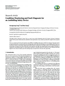
(4) Compute 𝑇2 and 𝑆𝑃𝐸 statistics of all training samples, and calculate the control limits 𝐿 𝑇2 and 𝐿 𝑆𝑃𝐸 , and then obtain the EWMA statistics and the control limit 𝐿 𝐸𝑊𝑀𝐴 . The online monitoring procedure is listed as follows: (1) Convert each testing sample into the high dimensional feature sample, and normalize the high dimensional feature samples 𝑥𝑛𝑒𝑤 with the mean and variance of the training feature samples 𝑥.. (2) Compute the kernel vector 𝐾𝑛𝑒𝑤 (𝑥, 𝑥𝑛𝑒𝑤 ) and center it to get 𝐾𝑛𝑒𝑤 (𝑥, 𝑥𝑛𝑒𝑤 ) via (23). (3) Calculate the projected vectors of testing samples 𝑦𝑛𝑒𝑤 via (41). (4) Compute EWMA statistics associated with 𝑥𝑛𝑒𝑤 , and judge whether they exceed the control limit 𝐿 𝐸𝑊𝑀𝐴 . The procedure of condition monitoring and fault detection by the method of NLKOPE is shown in Figure 1. The healthy vibration signals are collected to implement NLKOPE and construct the offline model, and then the model will be employed to implement online condition monitoring, fault detection, and performance degradation assessment.

5. Case Studies and Result Analysis 5.1. Fault Detection of Gearboxes. The 2009 PHM gearbox fault data [18] is a representative of generic industrial gearbox data; we use it to evaluate the proposed methods. The gearbox contains 4 gears, 6 bearings, and 3 shafts, the measured signals consist of two accelerometer signals and a tachometer signal with a sampling frequency of 66.67 kHz, and the schematic and overview of the gearbox are shown in Figure 2. In this study, 3 different health conditions of the helical gearbox under low load and 30 Hz speed are used to test the effect of fault detection, and the detailed description of the data and pattern is shown in Table 1. In the pattern of health, all the mechanical elements in the gearbox are normal. In the pattern of fault 1, the gear with 24 teeth on the idler shaft is chipped. In the pattern of fault 2, the gear with 24 teeth on the idler shaft is broken, and the bearing at output side of the idler shaft also has inner race defect. In this case, 1024 sampling points are selected as a sample, and we extract 30 samples for each pattern. The first 30 samples from the pattern of health are used as training samples, and the remaining 60 samples from pattern of fault 1

Shock and Vibration

7

Healthy vibration signals Training

Signal processing

Monitoring model: NLKOPE-EWMA

Offline model

Testing Vibration signals

High dimensional feature samples

Signal processing

Fault detection High dimensional feature samples

EWMA Degradation assessment

Online monitoring

Figure 1: Procedure of condition monitoring and fault detection.

Figure 2: Schematic and overview of the gearbox used in PHM 2009 Challenge Data [18].

Table 1: Pattern description of the gearbox: IS=input shaft;:IS=input side; ID=idler shaft;:OS=output Side; OS=output shaft. Pattern Health Fault 1 Fault 2

Gear 16T Good Good Good

48T Good Good Good

24T Good Chipped Broken

40T Good Good Good

IS:IS Good Good Good

ID:IS Good Good Good

Bearing OS:IS IS:OS Good Good Good Good Good Good

ID:OS Good Good Inner

OS:OS Good Good Good

Input Good Good Good

Shaft Output Good Good Good

8

Shock and Vibration Table 2: Fault detection rates of five methods.

FDR(%)

KPCA 90

KONPE 96.67

NLOPE 98.33

KGLPP [13] 98.33

Table 3: The clustering degree of different reduction algorithms. NLKOPE 100

and fault 2 are collected as testing samples. In other words, we use these 90 samples to detect whether the gearbox is faulty, and actually the gearbox starts to fail at 31st sample. For the purpose of comparison, five monitoring methods based on KPCA, KONPE, NLOPE, KGLPP [13], and NLKOPE are presented to detect the fault of gearbox respectively. The embedding dimension in each model is set to 3, and the number of nearest neighbors is set to 20 in KONPE, NLOPE, KGLPP, and NLKOPE models. The 99% confidence limit is used for 𝑇2 , 𝑆𝑃𝐸, and EWMA statistics. In order to compare the results more clearly, the indicator of fault detection rate (FDR) is applied in this case. Monitoring charts of five methods are shown in Figure 3, and the detailed fault detection results of these monitoring methods are listed in Table 2. Obviously, gearbox starts to fail at 33rd sample that detected by KPCA monitoring model as shown in Figure 3(a), and 35th, 36th, 37th, 38th samples are all under the control limit, that means the failure of detection at these samples. Figure 3(b) illustrates that gearbox starts to fail at 33rd sample that detected by KONPE, that means the failure of detection at 31st and 32nd samples. As shown in Figures 3(c)-3(d), gearbox starts to fail at 32nd sample that detected by NLOPE and KGLPP, but in fact, gearbox starts to fail at 31st sample. The detection result of NLKOPE monitoring model is shown in Figure 3(e); the EWMA statistic can work well and detect the fault of gearbox accurately. Besides, as shown in Table 2, the fault detection rates of NLOPE, KGLPP, and NLKOPE are higher than KPCA and KONPE which only consider the global or local data structure, although NLOPE has considered the global-local data information; the ability to process nonlinear data is not prominent when compared to NLKOPE. The results indicate that the NLKOPE-based monitoring method outperforms KPCA, KONPE, NLOPE, and KGLPP-based monitoring method. 5.2. Dimension Reduction Performance Assessment. In this case, the experimental data from Case Western Reserve University [23] are used to evaluate the dimension reduction performance of the proposed methods. The bearings used at the drive end are the deep groove ball bearing 6205-2RS JEM SKF. Data was collected with 12kHz sampling frequency at the rotating speed of 1797 rpm and 0HP load. The sample sets include 7 different severity conditions, i.e., health, inner race faults with faulty sizes 0.007, 0.014, 0.021, and 0.028, respectively, outer race, and ball fault with faulty size 0.014, respectively. We select 1024 sampling points as a sample, and extract 70 samples for each severity condition. Furthermore, the first 35 samples of each severity condition are collected as training samples, then the remaining 35 samples are used as testing samples. The purpose of dimension reduction is to make the intraclass low dimensional samples clustering and interclass

J

KPCA 0.0198

KONPE 0.0182

NLOPE 0.0185

KGLPP [13] 0.0102

NLKOPE 0.0088

separation, which will be helpful to improve the performance of fault classification. Thus, the clustering degree is used as a quantification index to evaluate the dimension reduction performance; it defines as follows: 𝐽= 𝑆𝑤 =

𝑆𝑤 𝑆𝑏

(42)

1 𝐶 𝑇 ∑ ∑ (𝑦 − 𝑚𝑖 ) (𝑦 − 𝑚𝑖 ) 𝑛𝑖 𝑖=1 𝑦∈𝐴 𝑖

𝐶

(43)

𝑇

𝑆𝑏 = ∑ (𝑚𝑖 − 𝑚) (𝑚𝑖 − 𝑚) 𝑖=1

where 𝐶 is the number of fault types, 𝑛𝑖 is the sample size of the 𝑖th fault type, 𝑦 is the low dimension embedded 𝑛 coordinate, 𝐴 𝑖 = (𝑦𝑖1 , ⋅ ⋅ ⋅ , 𝑦𝑖 𝑖 ), 𝑚𝑖 is the mean value of embedded coordinates of the 𝑖th fault type, and 𝑚 is the mean value of all low dimension embedded coordinates. 11 time-domain features and 13 frequency-domain features [21] are extracted from each sample to be the variations and make up the high dimensional sample, and in order to visualize clearly, the embedding dimension is set to 3. For the purpose of comparison, five methods including KPCA, KONPE, NLOPE, KGLPP [13], and NLKOPE are presented to obtain the dimension reduction results on the training and testing samples, respectively; scatter plots of three features are as shown in Figure 4. Furthermore, Health, Fault1, Fault2, Fault3, Fault4, Fault5, and Fault6 in Figure 4 represent 7 different fault types which contain health, four inner race faults with faulty sizes 0.007, 0.014, 0.021, and 0.028 in, outer race, and ball fault with faulty size 0.014 in, respectively, and x, y, z indicate three-dimensional representation based on the three features extracted from the training and testing samples by the proposed methods. Figure 4 illustrates the classification abilities of five methods for the 3D-clusters samples, where samples in the same fault types are marked in the same color. The distribution of the same fault type of samples is dispersed in Figure 4(a), and the different fault types of samples gather together as shown in Figure 4(b), both of these two situations may increase the probability of misclassification. The clustering degree is calculated as shown in Table 3, the clustering degree value of KGLPP is close to NLKOPE, and the result of dimension reduction based on NLKOPE has the minimum clustering degree, which is beneficial to improve the accuracy of fault classification. 5.3. Condition Monitoring and Performance Degradation Assessment of Bearing. In this case, the aim is to implement condition monitoring and evaluate the performance degradation of bearing, and the degradation index is important to assess the state of bearing. Thus, we hope to identify the

9

0.8

0.8

0.7

0.7

0.6

0.6

0.5

0.5

0.4

EWMA

EWMA

Shock and Vibration

number of fault start: 33

0.4

0.3

0.3

0.2

0.2

0.1

0.1

0

20

40

60

number of fault start: 33

0

80

20

40 Samples

Samples (a) Fault detection result using KPCA

60

80

(b) Fault detection result using KONPE

0.5

0.35 0.3

0.4

EWMA

0.3

0.2 number of fault start: 32

0.2 number of fault start: 32 0.15 0.1

0.1 0.05 0

20

40 Samples

60

0

80

20

(c) Fault detection result using NLOPE

40 Samples

60

(d) Fault detection result using KGLPP

0.5

0.4

EWMA

EWMA

0.25

0.3

0.2 number of fault start: 31 0.1

0

20

40 Samples

60

80

(e) Fault detection result using NLKOPE

Figure 3: Monitoring charts: (a) KPCA, (b) KONPE, (c) NLOPE, (d) KGLPP, and (e) NLKOPE.

80

10

Shock and Vibration

1

5

z

z

0.5 0

0 −0.5 1

−5 10

1 y

0 0

−1 −0.5 Health Fault1 Fault2 Fault3

5

0.5

5 y

x

0

0 −5

Health Fault1 Fault2 Fault3

Fault4 Fault5 Fault6 Testing samples

Fault4 Fault5 Fault6 Testing samples (b)

4

1.5

2

1

0

0.5

z

z

(a)

−2

0

−4 5

−0.5 4 y

0

0

2

2

−2

−5 −4 Health Fault1 Fault2 Fault3

x

−5

y x

Fault4 Fault5 Fault6 Testing samples

0 −2

−4

x

Fault4 Fault5 Fault6 Testing samples

Health Fault1 Fault2 Fault3

(c)

−2

0

(d)

2

z

0 −2 −4 5 y

5

0

0 −5 −5

Health Fault1 Fault2 Fault3

x

Fault4 Fault5 Fault6 Testing samples (e)

Figure 4: Three-dimensional representation based on the three features extracted from the training and testing samples by (a) KPCA, (b) KONPE, (c) NLOPE, (d) KGLPP, and (e) NLKOPE.

Shock and Vibration

11 1.4 severe degradation 1.2 1797

EWMA

1 weak degradation beginning

0.8 0.6 0.4 0.2 0

500

1000 Samples

1500

2000

Figure 6: Monitoring chart by KPCA.

1.4 severe degradation 1.2 1

Figure 5: Bearing test rig [19]. Figure 5 is reproduced from H. Qiu et al. (2006).

EWMA

1797 0.8 weak degradation beginning

0.6 0.4

degradation at an early stage to avoid continuous deterioration of the state and minimize machine downtime. The bearing experimental data were generated from the runto-failure test [19, 24]. Figure 5 illustrates the bearing test rig. The rotation speed was kept constant at 2000 rpm, and each sample consists of 20480 points with the sampling rate set at 20kHz. The structural parameters and kinematical parameters (shaft frequency 𝑓𝑟 , inner-race fault frequency 𝑓𝑖 , rolling element fault frequency 𝑓𝑏 , and outer-race fault frequency 𝑓𝑜 ) of the experiment bearing are listed in Table 4, and the detailed information about the experiments have been introduced in the literature [19]. One bearing (i.e., the bearing 3 of testing 1) with inner race defect is used to verify the performance of the proposed algorithm. We extract 2100 sets of test-to-fail samples recorded for the bearing 3, the first 500 samples are used as the training samples, and the rest are generated as the testing samples. For the purpose of comparison, five monitoring methods based on KPCA, KONPE, NLOPE, KGLPP [13], and NLKOPE are presented to explain the bearing performance state, respectively. The 99% confidence limit is used for 𝑇2 , 𝑆𝑃𝐸, and EWMA statistics. In this case, we extracted 2100 test-to-fail samples, and the 1790th sample was regarded as the initial weak degradation point based on the research in literature [25]. As shown in Figures 6 and 7, the EWMA statistic has presented the state of the bearing, and the 1797th sample is considered to be the initial weak degradation point where the performance of the bearing begins to degrade. As the

0.2 0

500

1000 Samples

1500

2000

Figure 7: Monitoring chart by KONPE.

samples were recorded every ten minutes, it is 70 minutes late to detect the failure by KPCA or KONPE-based monitoring method when compared with the result in literature [25], and the KPCA-EWMA statistic with large fluctuations is not suitable for condition monitoring. Figures 8–10 illustrate the detection results of NLOPE, KGLPP, and NLKOPEbased monitoring methods, and they all obtain the initial weak degradation point of the bearing at the 1789th sample, which is 10 minutes earlier than the result in literature [25], and the statistics after 1789th sample all exceed the control limits, but LPP-EWMA statistics [25] between 1950th sample and 2150th sample are below the control limit, that means the failure of detection in these interval. Though the fault detection accuracy of NLOPE-based monitoring method outperforms KPCA and KONPE, this advantage of NLOPE is not prominent, since the EWMA statistic after the initial weak degradation point has a relative big fluctuation as shown in Figure 8, which is not conducive to evaluating the bearing performance state. The performance degradation assessment of KGLPP-based monitoring method is slightly

12

Shock and Vibration Table 4: Structural parameters and kinematical parameters of the experiment bearing.

Number of rolling elements 16 𝑓𝑟 (Hz) Characteristic frequency 33 Bearing designation

Diameter of the pitch (in.) 2.815 𝑓𝑖 (Hz) 296.9

0.35

Contact angle 15.17∘ 𝑓𝑏 (Hz) 279.8

Diameter of the rolling element (in.) 0.331 𝑓0 (Hz) 236.4

0.01

0.3 0.008

0.2

EWMA

EWMA

0.25

0.15 0.1

1789

0.006

0.004

1789

0.002

weak degradation beginning

0.05 0

500

1000 Samples

1500

0 1650

2000

1700

(a)

1750 Samples

1800

1850

(b)

Figure 8: Monitoring charts by NLOPE: (a) EWMA statistic; (b) local enlargement of (a).

1.4

1.5

severe degradation

severe degradation

1.2 1 1789 EWMA

EWMA

1 1789

0.8 0.6

weak degradation beginning

weak degradation beginning

0.5

0.4 0.2 0

500

1000 Samples

1500

2000

0

500

1000

1500

2000

Samples

Figure 9: Monitoring chart by KGLPP.

Figure 10: Monitoring chart by NLKOPE.

inferior to the performance of NLKOPE-based monitoring method, because NLKOPE-EWMA statistic can reflect the damage degree of the bearing from the severe degradation occurrence of incipient defect to final failure, as shown in Figure 10, the EWMA statistic continues to grow from severe degradation to final failure stage, which is consistent with actual bearing degradation. Thus we can draw the conclusion that the NLKOPE-based monitoring model which considers the global and local data structure together will obtain better monitoring performance than the model considering only the global structure or local structure of data.

The above results have shown that the proposed method can be effectively used for the task of bearing fault detection. The next step is to diagnose the fault type of the bearing. We extract the 1789th sample to analysis, the signal is complex and messy that contains lots of noise as shown in Figure 11, and thus it is hard to diagnose whether the bearing is faulty only by the time waveform of the vibration signal, as the features have been submerged by the strong noise. In order to extract useful features for diagnosis, it is necessary to eliminate the noise in the original vibration signal. Dualtree complex wavelet packet transform (DTCWPT) is a

13

0.6

0.4

0.4

0.3

0.2

0.2 Amplitude[m/Ｍ2 ]

Amplitude[m/Ｍ2 ]

Shock and Vibration

0 −0.2 −0.4

0.1 0 −0.1

−0.6

−0.2

−0.8

−0.3

−1

0

0.02

0.04

0.06 Time[s]

0.08

−0.4

0.1

0

0.02

0.06

0.08

0.1

Time[s]

Figure 11: Time waveform of vibration signal.

Figure 12: Time waveform of denoised vibration signal.

0.014

＠Ｌ

0.012

3＠ Ｌ 2＠ Ｌ

0.01 Amplitude[/]

multiscale method with such attractive properties as nearly shift-invariance and reduced aliasing, which has been widely used in signal processing [26]. In this study, DTCWPT is employed to denoise the original vibration signal combined with the threshold method, and Hilbert transform envelope algorithm is applied to extract the fault characteristic frequency. As shown in Figure 12, the noise in vibration signal has been greatly reduced, and transient periodicity can be found because of the impacts produced by the bearing defect. The envelop spectrum of denoised vibration signal is presented in Figure 13, we can find the shaft frequency 𝑓𝑟 and its harmonics, the fault characteristic frequency 𝑓𝑖 and its harmonics are all quite effectively extracted, and there are also side bands 𝑓1 and 𝑓2 on both sides of the fault characteristic frequency 𝑓𝑖 . Therefore, the bearing inner race can be judged to be faulty, which is also in line with the actual condition of the bearing.

0.04

＠1

0.008

＠i

＠2 2＠ i 3＠ i

0.006 0.004 0.002 0

0

200

400 600 Frequency[Hz]

800

1000

Figure 13: Envelop spectrum of denoised vibration signal.

6. Conclusions In this paper, a linear dimension reduction method called nonlocal orthogonal preserving embedding is proposed, and the nonlinear form of NLOPE named nonlocal kernel orthogonal preserving embedding is also presented. In order to retain the geometric of the latent manifold, NLOPE and NLKOPE both take global and local data structures into account, and a tradeoff parameter is introduced to balance the global preserving and local preserving. Hence, compared to KPCA and KONPE, NLKOPE is more general and flexible, and it is also more powerful to extract latent information from nonlinear data than NLOPE. Based on the results of three cases, the dimension reduction performance of NLKOPE is the best, which is beneficial to improve the accuracy of fault classification, and NLKOPE-based monitoring method has higher fault detection rate, it is also more sensitive and effective to evaluate the performance degradation of bearing in comparison with KPCA, KONPE, and NLOPEbased monitoring method.

Appendix A. To obtain the result of 𝑎1 , we construct the Lagrange function of 𝐿(𝑎1 ) based on (24) 𝐿 (𝑎1 ) = 𝑎1𝑇 [𝜂𝑥𝑀𝑥𝑇 − (1 − 𝜂) 𝐶] 𝑎1 − 𝜆 {𝑎1𝑇 [𝜂𝑥𝑥𝑇 + (1 − 𝜂) 𝐼] 𝑎1 − 1}

(A.1)

Let 𝑆 = 𝜂𝑥𝑥𝑇 + (1 − 𝜂)𝐼, 𝐷 = 𝜂𝑥𝑀𝑥𝑇 − (1 − 𝜂)𝐶, set the partial derivative of 𝐿(𝑎1 ) with respect to 𝑎1 to be zero, and we get 𝜕𝐿 (𝑎1 ) = 2𝐷𝑎1 − 2𝜆𝑆𝑎1 = 0 𝜕𝑎1

(A.2)

Thus, 𝑎1 is the eigenvector corresponding to the smallest eigenvalue of matrix 𝑆−1 𝐷.

14

Shock and Vibration

To obtain the result of 𝑎𝑘 , we construct the Lagrange function of 𝐿(𝑎𝑘 ) based on (24) 𝐿 (𝑎𝑘 ) = 𝑎𝑘𝑇 [𝜂𝑥𝑀𝑥𝑇 − (1 − 𝜂) 𝐶] 𝑎𝑘 − 𝜆 {𝑎𝑘𝑇 [𝜂𝑥𝑥𝑇 + (1 − 𝜂) 𝐼] 𝑎𝑘 − 1}

(A.3)

B. To obtain the result of 𝑎1 , we construct the Lagrange function of 𝐿(𝑎1 ) based on (31) 𝐿 (𝑎1 ) =

𝑇 𝑎1𝑇 [𝜂𝐾 𝑀𝐾

𝑘−1

− ∑ 𝑢𝑖 𝑎𝑘𝑇 𝑎𝑖

−

𝑖=1

𝑘−1

𝐿 (𝑎𝑘 ) = 𝑎𝑘𝑇 𝐷𝑎𝑘 − 𝜆 (𝑎𝑘𝑇 𝑆𝑎𝑘 − 1) − ∑ 𝑢𝑖 𝑎𝑘𝑇𝑎𝑖

(A.4)

𝑖=1

Set the partial derivative of 𝐿(𝑎𝑘 ) with respect to 𝑎𝑘 to be zero 𝑘−1 𝜕𝐿 (𝑎𝑘 ) = 2𝐷𝑎𝑘 − 2𝜆𝑆𝑎𝑘 − ∑ 𝑢𝑖 𝑎𝑖 = 0 𝜕𝑎𝑘 𝑖=1

(A.5)

Multiplying the left side of (A.4) by 𝑎𝑖𝑇𝑆−1 , we have 𝑎𝑖𝑇 𝑆−1 ∑ 𝑢𝑖 𝑎𝑖 = 2𝑎𝑖𝑇𝑆−1 𝐷𝑎𝑘

(A.6)

𝑖=1

𝑖 = 1, 2, ⋅ ⋅ ⋅ , 𝑘 − 1, (A.6) can be represented as 𝑎1𝑇 𝑢1 [ ] ] [ [ .. ] −1 [ .. ] [ . ] 𝑆 [𝑎1 , ⋅ ⋅ ⋅ , 𝑎𝑘−1 ] [ . ] [ ] ] [ 𝑇 [𝑎𝑘−1 ] [𝑢𝑘−1]

𝜕𝐿 (𝑎1 ) = 2𝐷𝑎1 − 2𝜆𝑆𝑎1 = 0 𝜕𝑎1

(B.2)

Thus, 𝑎1 is the eigenvector corresponding to the smallest eigenvalue of matrix 𝑆−1 𝐷. To obtain the result of 𝑎𝑘 , we construct the Lagrange function of 𝐿(𝑎𝑘 ) based on (31)

=

𝑇 𝑎𝑘𝑇 [𝜂𝐾 𝑀𝐾

𝑇

𝐾 𝐾 ] 𝑎𝑘 − (1 − 𝜂) 𝑁 𝑇

𝑘−1

(B.3)

𝑇

𝑖=1

(A.7)

Substituting 𝑆 and 𝐷 into (B.3) and setting the partial derivative of 𝐿(𝑎𝑘 ) with respect to 𝑎𝑘 to be zero, we obtain 𝑘−1

𝑇

𝐿 (𝑎𝑘 ) = 𝑎𝑘𝑇 𝐷𝑎𝑘 − 𝜆 (𝑎𝑘𝑇𝑆𝑎𝑘 − 1) − ∑ 𝑢𝑖 𝑎𝑘𝑇 𝐾 𝑎𝑖

(B.4)

𝑖=1

Let 𝑢(𝑘−1) = [𝑢1 , 𝑢2 , ⋅ ⋅ ⋅ , 𝑢𝑘−1 ]𝑇, 𝑎(𝑘−1) = [𝑎1 , 𝑎2 , ⋅ ⋅ ⋅ , 𝑎𝑘−1 ], we obtain −1

𝑇

𝑢(𝑘−1) = 2 [(𝑎(𝑘−1) ) 𝑆−1 𝑎(𝑘−1) ] (𝑎(𝑘−1) ) 𝑆−1 𝐷𝑎𝑘

(A.8)

Multiplying (A.4) by 𝑆−1 and substituting (A.8), we obtain −1

(A.9)

⋅ 𝑆−1 𝐷𝑎𝑘 = 𝜆𝑎𝑘 Thus, 𝑎𝑘 is the eigenvector corresponding to the smallest eigenvalue of matrix 𝑄(𝑘) : 𝑄(𝑘) = {𝐼 − (𝑆)−1 𝑎(𝑘−1) [(𝑎(𝑘−1) ) (𝑆)−1 𝑎(𝑘−1) ]

𝑘−1 𝜕𝐿 (𝑎𝑘 ) 𝑇 = 2𝐷𝑎𝑘 − 2𝜆𝑆𝑎𝑘 − ∑ 𝑢𝑖 𝐾 𝑎𝑖 = 0 𝜕𝑎𝑘 𝑖=1

(B.5)

Multiplying the left side of (B.4) by 𝑎𝑖𝑇 𝑆−1 , we have 𝑘−1

𝑇

𝑎𝑖𝑇𝑆−1 ∑ 𝑢𝑖 𝐾 𝑎𝑖 = 2𝑎𝑖𝑇 𝑆−1 𝐷𝑎𝑘

(B.6)

𝑖=1

𝑇

{𝐼 − 𝑆−1 𝑎(𝑘−1) [(𝑎(𝑘−1) ) 𝑆−1 𝑎(𝑘−1) ] (𝑎(𝑘−1) ) }

𝑇

𝑇

Let 𝑆 = 𝜂(𝐾 𝐾 + 𝐾) + (1 − 𝜂)𝐼, 𝐷 = 𝜂𝐾 𝑀𝐾 − (1 − 𝑇 𝜂)𝐾 𝐾/𝑁, set the partial derivative of 𝐿(𝑎1 ) with respect to 𝑎1 to be zero, we get

− 𝜆 {𝑎𝑘𝑇 [𝜂 (𝐾 𝐾 + 𝐾) + (1 − 𝜂) 𝐼] 𝑎𝑘 − 1}

[ ] [ ] = 2 [ ... ] 𝑆−1 𝐷𝑎𝑘 [ ] 𝑇 𝑎 [ 𝑘−1 ]

⋅ (𝑎(𝑘−1) ) } 𝑆−1 𝐷

+ 𝐾) + (1 − 𝜂) 𝐼] 𝑎1 − 1}

− ∑ 𝑢𝑖 𝑎𝑘𝑇 𝐾 𝑎𝑘

𝑎1𝑇

𝑇

(B.1)

𝐿 (𝑎𝑘 )

𝑘−1

𝑇

𝑇 𝜆 {𝑎1𝑇 [𝜂 (𝐾 𝐾 𝑇

Substituting 𝑆 and 𝐷 into (A.3), we get

𝑇

𝑇

𝐾 𝐾 ] 𝑎1 − (1 − 𝜂) 𝑁

−1

𝑖 = 1, 2, ⋅ ⋅ ⋅ , 𝑘 − 1, (B.6) can be represented as 𝑎1𝑇 𝑢1 [ ] ] [ 𝑇 [ .. ] −1 [ . ] [ . ] 𝑆 𝐾 [𝑎1 , ⋅ ⋅ ⋅ , 𝑎𝑘−1 ] [ .. ] [ ] ] [ 𝑇 𝑢 𝑎 [ 𝑘−1 ] [ 𝑘−1 ] 𝑎1𝑇

(A.10)

[ ] [ ] = 2 [ ... ] 𝑆−1 𝐷𝑎𝑘 [ ] 𝑇 [𝑎𝑘−1 ]

(B.7)

Shock and Vibration

15

Let 𝑢(𝑘−1) = [𝑢1 , 𝑢2 , ⋅ ⋅ ⋅ , 𝑢𝑘−1 ]𝑇, 𝑎(𝑘−1) = [𝑎1 , 𝑎2 , ⋅ ⋅ ⋅ , 𝑎𝑘−1 ], and we obtain 𝑢(𝑘−1) 𝑇

𝑇

−1

𝑇

= 2 [(𝑎(𝑘−1) ) 𝑆−1 𝐾 𝑎(𝑘−1) ] (𝑎(𝑘−1) ) 𝑆−1 𝐷𝑎𝑘

(B.8)

Multiplying (B.4) by 𝑆−1 and substituting (B.8), we obtain 𝑇

𝑇

𝑇

{𝐼 − 𝑆−1 𝐾 𝑎(𝑘−1) [(𝑎(𝑘−1) ) 𝑆−1 𝐾 𝑎(𝑘−1) ]

(B.9)

(𝑘−1) 𝑇

⋅ (𝑎

−1

−1

) } 𝑆 𝐷𝑎𝑘 = 𝜆𝑎𝑘

Thus, 𝑎𝑘 is the eigenvector corresponding to the smallest eigenvalue of matrix 𝑄(𝑘) : 𝑇

𝑇

𝑇

𝑄(𝑘) = {𝐼 − 𝑆−1 𝐾 𝑎(𝑘−1) [(𝑎(𝑘−1) ) 𝑆−1 𝐾 𝑎(𝑘−1) ] (𝑘−1) 𝑇

⋅ (𝑎

−1

(B.10) −1

) }𝑆 𝐷

Conflicts of Interest The authors declare that they have no conflicts of interest.

Acknowledgments This research is supported by National Nature Science Foundation of China (nos. 61640308 and 61573364) and Nature Science Foundation of Naval University of Engineering (no. 20161579). The author is also grateful to the 2009 PHM Challenge Competition, Case Western Reserve University, and NSF I/UCR Center for Intelligent Maintenance System, University of Cincinnati, USA, for providing the experimental data.

References [1] Q. Jiang, X. Yan, and B. Huang, “Performance-driven distributed PCA process monitoring based on fault-relevant variable selection and bayesian inference,” IEEE Transactions on Industrial Electronics, vol. 63, no. 1, pp. 377–386, 2016. [2] S. J. Qin, “Survey on data-driven industrial process monitoring and diagnosis,” Annual Reviews in Control, vol. 36, no. 2, pp. 220–234, 2012. [3] Z. Ge, “Review on data-driven modeling and monitoring for plant-wide industrial processes,” Chemometrics and Intelligent Laboratory Systems, vol. 171, pp. 16–25, 2017. [4] Z. Ge, C. Yang, and Z. Song, “Improved kernel PCA-based monitoring approach for nonlinear processes,” Chemical Engineering Science, vol. 64, no. 9, pp. 2245–2255, 2009. [5] M. Yao and H. Wang, “On-line monitoring of batch processes using generalized additive kernel principal component analysis,” Journal of Process Control, vol. 28, pp. 56–72, 2015. [6] M. Zhang, Z. Ge, Z. Song, and R. Fu, “Global–Local Structure Analysis Model and Its Application for Fault Detection and Identification,” Industrial & Engineering Chemistry Research, vol. 50, no. 11, pp. 6837–6848, 2011.

[7] M. Belkin and P. Niyogi, “Laplacian eigenmaps for dimensionality reduction and data representation,” Neural Computation, vol. 15, no. 6, pp. 1373–1396, 2003. [8] X. He and P. Niyogi, “Locality preserving projections,” Advances in Neural Information Processing Systems, vol. 16, pp. 153–160, 2004. [9] S. T. Roweis and L. K. Saul, “Nonlinear dimensionality reduction by locally linear embedding,” Science, vol. 290, no. 5500, pp. 2323–2326, 2000. [10] X. He, D. Cai, S. Yan, and H. Zhang, “Neighborhood preserving embedding,” in Proceedings of the 10th IEEE International Conference on Computer Vision (ICCV ’05), pp. 1208–1213, Beijing, China, October 2005. [11] J. Yu, “Local and global principal component analysis for process monitoring,” Journal of Process Control, vol. 22, no. 7, pp. 1358–1373, 2012. [12] J. Wang, J. Feng, and Z. Y. Han, “Locally preserving PCA method based on manifold learning and its application in fault detection,” Control and Decision, vol. 22, no. 5, pp. 683–687, 2013. [13] L. Luo, S. Bao, J. Mao, and D. Tang, “Nonlinear process monitoring based on kernel global-local preserving projections,” Journal of Process Control, vol. 38, pp. 11–21, 2016. [14] L. J. Luo, “Process Monitoring with Global–Local Preserving Projections,” American Chemical Society, vol. 53, no. 18, pp. 7696–7705, 2014. [15] X. Liu, J. Yin, Z. Feng, J. Dong, and L. Wang, “Orthogonal neighborhood preserving embedding for face recognition,” in Proceedings of the 14th IEEE International Conference on Image Processing, ICIP 2007, pp. I133–I136, usa, September 2007. [16] D. Cai, X. He, J. Han, and H.-J. Zhang, “Orthogonal laplacianfaces for face recognition,” IEEE Transactions on Image Processing, vol. 15, no. 11, pp. 3608–3614, 2006. [17] J.-D. Shao, G. Rong, and J. M. Lee, “Generalized orthogonal locality preserving projections for nonlinear fault detection and diagnosis,” Chemometrics and Intelligent Laboratory Systems, vol. 96, no. 1, pp. 75–83, 2009. [18] Phm data challenge 2009, http://www.phmsociety.org/competition/PHM/09. [19] H. Qiu, J. Lee, J. Lin, and G. Yu, “Wavelet filter-based weak signature detection method and its application on rolling element bearing prognostics,” Journal of Sound and Vibration, vol. 289, no. 4-5, pp. 1066–1090, 2006. [20] F. He and J. Xu, “A novel process monitoring and fault detection approach based on statistics locality preserving projections,” Journal of Process Control, vol. 37, pp. 46–57, 2016. [21] Y. Lei, Z. He, and Y. Zi, “A new approach to intelligent fault diagnosis of rotating machinery,” Expert Systems with Applications, vol. 35, no. 4, pp. 1593–1600, 2008. [22] J.-H. Cho, J.-M. Lee, S. W. Choi, D. Lee, and I.-B. Lee, “Fault identification for process monitoring using kernel principal component analysis,” Chemical Engineering Science, vol. 60, no. 1, pp. 279–288, 2005. [23] K. A. Loparo, Bearings Vibration Data Set, Case Western Reserve University, 2003, http://csegroups.case.edu/bearingdatacenter/pages/apparatus-procedures. [24] J. Lee, H. Qiu, G. Yu, and J. Lin, Bearing Data Set. IMS, University of Cincinnati. NASA Ames Prognostics Data Repository, NASA Ames, Moffett Field, CA, USA, http://dataacoustics.com/measurements/bearing-faults/bearing-4.

16 [25] J.-B. Yu, “Bearing performance degradation assessment using locality preserving projections,” Expert Systems with Applications, vol. 38, no. 6, pp. 7440–7450, 2011. [26] J. Qu, Z. Zhang, and T. Gong, “A novel intelligent method for mechanical fault diagnosis based on dual-tree complex wavelet packet transform and multiple classifier fusion,” Neurocomputing, vol. 171, no. 1, pp. 837–853, 2016.

Shock and Vibration

International Journal of

Advances in

Rotating Machinery

Engineering Journal of

Hindawi www.hindawi.com

Volume 2018

The Scientific World Journal Hindawi Publishing Corporation http://www.hindawi.com www.hindawi.com

Volume 2018 2013

Multimedia

Journal of

Sensors Hindawi www.hindawi.com

Volume 2018

Hindawi www.hindawi.com

Volume 2018

Hindawi www.hindawi.com

Volume 2018

Journal of

Control Science and Engineering

Advances in

Civil Engineering Hindawi www.hindawi.com

Hindawi www.hindawi.com

Volume 2018

Volume 2018

Submit your manuscripts at www.hindawi.com Journal of

Journal of

Electrical and Computer Engineering

Robotics Hindawi www.hindawi.com

Hindawi www.hindawi.com

Volume 2018

Volume 2018

VLSI Design Advances in OptoElectronics International Journal of

Navigation and Observation Hindawi www.hindawi.com

Volume 2018

Hindawi www.hindawi.com

Hindawi www.hindawi.com

Chemical Engineering Hindawi www.hindawi.com

Volume 2018

Volume 2018

Active and Passive Electronic Components

Antennas and Propagation Hindawi www.hindawi.com

Aerospace Engineering

Hindawi www.hindawi.com

Volume 2018

Hindawi www.hindawi.com

Volume 2018

Volume 2018

International Journal of

International Journal of

International Journal of

Modelling & Simulation in Engineering

Volume 2018

Hindawi www.hindawi.com

Volume 2018

Shock and Vibration Hindawi www.hindawi.com

Volume 2018

Advances in

Acoustics and Vibration Hindawi www.hindawi.com

Volume 2018