Chen J.C.: Measured Performance of 5-GHz 802.11a Wireless LAN Systems, Atheros. Communications white paper, 2001. 6. Williams H.P.: Model building in ...
Nonlinear Optimization of IEEE 802.11 Mesh Networks Enrique Costa-Montenegro, Francisco J. Gonz´ alez-Casta˜ no, Pedro S. Rodr´ıguez-Hern´andez, and Juan C. Burguillo-Rial Departamento de Ingenier´ıa Telem´ atica, Universidad de Vigo, Spain {kike,javier,pedro,jrial}@det.uvigo.es http://www-gti.det.uvigo.es
Abstract. In this paper, we propose a novel optimization model to plan IEEE 802.11 broadband access networks. From a formal point of view, it is a mixed integer non-linear optimization model that considers both co-channel and inter-channel interference in the same compact formulation. It may serve as a planning tool by itself or to provide a performance bound to validate simpler planning models such as those in [3]. Keywords: IEEE 802.11, mesh networks, rooftop, planning.
1
Introduction
In this paper, we propose an optimization model to generate IEEE 802.11 resource-sharing broadband access meshes, which users themselves often manage [1]. Resource-sharing wireless networks based on IEEE 802.11 are not new [2]. In our model, a basic node is composed by a cable/xDSL router, an 802.11 access point and two 802.11 cards for interworking purposes. Basic nodes may serve a LAN (covering a building, for example). This model may represent user-managed rooftop networks linking building LANs, to share a pool of cable/xDSL accesses. Our proposal relies on a set of rules to generate topologies with low co-channel and inter-channel interference. From them, in a previous paper [3] we derived two mesh deployment algorithms: a distributed one, to be executed by infrastructure nodes themselves, and a centralized one via a mixed integer linear optimization model. In this paper we enrich the centralized version, by adding co-channel and inter-channel interference estimates that yield a mixed integer non-linear optimization model. The new model may serve as a planning tool or to provide a performance bound to validate previous planning models. Our study is based on IEEE 802.11b because it has been the most extended legal 802.11 substandard in the EU for a long time. It is straightforward to extend the results of this work to other substandards like IEEE 802.11a or 802.11g. This paper is organized as follows: section 2 reviews the work in [3]. Section 3 describes the new proposal, a mixed integer non-linear optimization model satisfying the deployment rules in [3]. Section 4 presents numerical tests on a realistic scenario –a sector in Vigo, Spain–. Section 5 concludes. Y. Shi et al. (Eds.): ICCS 2007, Part IV, LNCS 4490, pp. 466–473, 2007. c Springer-Verlag Berlin Heidelberg 2007 �
Nonlinear Optimization of IEEE 802.11 Mesh Networks
2
467
Distributed IEEE 802.11 Deployment Algorithm
A single access point per basic node is a natural choice, since it can manage connections from several wireless cards. Multiple access points per basic node would compromise cell planning, due to the few channels available. According to our previous work, two wireless cards per basic node yield satisfactory performance and ensure network diversity and survivability. 2.1
IEEE 802.11b Channel Assignment
IEEE 802.11b has 13 DSSS (Direct Sequence Spread Spectrum) overlapping channels. We wish to minimize co-channel and inter-channel interference in wireless infrastructure deployment. There is co-channel interference when two access points (AP) employ the same channel, and inter-channel interference when APs or wireless cards (WLCs) with overlapping channels transmit simultaneously. We adopt the classic cellular planning algorithm in [4] to generate a channel grid (Figure 1). We assign AP channels according to the cells they belong to. The maximum legal range (without boosting equipment) of card-to-access point connections is 170 meters (using a D-Link DWL-1000 AP and D-Link DWL-650 WLCs). IEEE 802.11b co-channel interference is negligible at distances over 50 m [5]. To mitigate co-channel and inter-channel interference, we allow a single fully active basic node per cell (the rest become partially active, by disabling the AP and one of the WLCs) and set cell edge length to 50 meters.
Fig. 1. Frequency pattern and cell grid
If there are several basic nodes in a cell, we need to decide which one is active. We achieved the lowest interference level when the active node is close to the cell center. Note that all basic nodes in a cell but the active one could be WLCs to reduce costs. However, this solution restricts network evolution (basic nodes can appear and disappear). Also, note that the cost per user is very low if the basic node serves a LAN. 2.2
Setting Wireless Links
As soon as a basic node is active, its WLCs look for the closest AP (in signal strength), i.e. the local one. The basic nodes filter the MAC addresses of their
468
E. Costa-Montenegro et al.
own WLCs. However, once a WLC in basic node A is connected to the AP in basic node B, the latter must block the second card in A, since (i) overall capacity is the same due to AP sharing and (ii) there would be less diversity otherwise. It is possible to detect and avoid this one-way dual connection establishment problem because both WLCs in A belong to the same addressing range. When a WLC wants to join the AP in a remote basic node, the latter must check if any of its WLCs have previously set a link in the opposite direction. The requesting WLC must notify its IP range, and the remote basic node can check if any of its own WLCs already belongs to that range (two-way dual connection establishment problem). If so, it will deny the connection. In zones with many basic nodes, another connection establishment problem arises when some of them handle many connections. However, it is possible to limit the number of connections per AP at IEEE 802.11b MAC level by blocking association request frames from WLCs once the connection counter reaches the limit, keeping a reasonable throughput per connection. This has a second beneficial effect, because it favors network expansion at its edges. We now consider co-channel and inter-channel interference. The former is presumably low due to cellular planning and cell size, specially if inter-cell links are short. Regarding inter-channel interference, if two physically adjacent IEEE 802.11b sources transmit with a two-channel separation, throughput drops to 50%, whereas a three-channel separation is practically enough to avoid interchannel interference. It may be quite common in our case. Thus, we consider an inter-channel interference mitigation rule. If implemented, all elements in a basic node (WLCs and AP) only set connections with mutual frequency separation of at least three channels. This drastically reduces inter-channel interference. 2.3
Performance of the Distributed Deployment Algorithm
In [3], we simulated the distributed deployment algorithm on a realistic scenario with a significant number of basic nodes (≈ 50), corresponding to Vigo, Spain. We observed that most WLCs got connected and the resulting mesh had link diversity. Figure 2(a) shows the resulting network: black icons represent fully active basic nodes, and “×” icons denote partially active ones (6 out of 46). Access point degree is low: 2.11. At the solution, there are some unconnected APs and WLCs. This is not evident in figure 2(a), because the corresponding basic nodes are not isolated. This does not imply a waste of network resources, since those cases are mainly located at mesh edges, and thus they allow future growth. Also, over 50% APs have at most two connections, which implies a high throughput per connection. Practically all WLCs set connections (97.8%). The percentage of highest-rate links (11 Mbps) is close to 90%.
3
Improved IEEE 802.11 Deployment Algorithm
In [3], we proposed a centralized deployment algorithm based on a mixed integer linear program. Now we present a new mesh planning model that adds explicit counter-interference constraints, which is a mixed integer non-linear program.
Nonlinear Optimization of IEEE 802.11 Mesh Networks
469
Fig. 2. Vigo: (a) Network example, (b) New algorithm with 25% frozen connections
Due to the complexity of this nonlinear model, our solver could not handle it on a Pentium IV desktop. So we decided to break it to solve it iteratively, as explained in section 4. In the next subsections we describe our model. 3.1
Sets and Constants
The main set BN contains N basic nodes bi , i = 0, . . . , N − 1. This set is divided into two disjoint subsets, BNf (fully active basic nodes) and BNp (partially active basic nodes). Thus, BNp ∩BNf = ∅ and BN = BNp ∪BNf . Let dij indicate the distance between bi and bj , kij the capacity of the corresponding link, and ch api the channel of the AP in node bi . If it is partially active, ch api =0. If it is fully active, ch api is the channel index of bi plus two. Consequently, ch api is 0 or an integer in [3, 15]. 3.2
Variables
Let i, j = 0, . . . , N − 1. The variables in the model are: – c1ij , c2ij : Boolean variables. They equal 1 if WLCs #1 or #2 in bi are connected to the AP in bj , respectively. They equal 0 otherwise. – ch w1i , ch w2i : real variables indicating the channels that WLCs #1 and #2 in bi acquire once connected. The optimization model ensures that they will take integer values (see condition C6 and remark 1). – δi : Boolean variable. If WLC #1 in bi is not connected, it equals 1 to set ch w1i to dummy channel 18. Dummy channel 18 allows to set constraints (7)-(9) representing the inter-channel interference rule (remark 2). – ei , fi : Boolean variables, to define linear constraints (8) and (9) that enforce the inter-channel interference mitigation rule in a fully active node bi (remark 2). – conex api : real variable, number of connections received by bi . Values in [0,4]. – capi : real variable, aggregated capacity of the connections received by basic node i. – cap poni : real variable, average capacity of the connections bond to the AP in bi . – degrki : real variable, degradation in bi due to links transmitting in channels with mutual distance k. – perc dki : real variable, indicating the percentage of capacity waste due to interference in basic node i by channels with mutual distance k.
470
3.3
E. Costa-Montenegro et al.
Conditions
From mesh design specifications, we impose a series of conditions on model variables. The optimization tools take advantage of these conditions to reduce model size and execution time drastically. Let bi , bj be basic nodes in BN . Let bp be a basic node in BNp . Then: c1ip , c2ip = 0, since partially active nodes do not have APs. c2pi = 0, since WLC #2 is disabled in partially active nodes. kij = 0 ⇒ c1ij , c2ij = 0: no connections between nodes that are far apart. c1ii , c2ii = 0, connections are forbidden within the same basic node. | ch api − ch apj | < 3 ⇒ c1ij , c2ij = 0, due to the inter-channel interference mitigation rule. To understand this, suppose that | ch api − ch apj | < 3 and c1ij = 1 or c2ij = 1 . If so, one of the WLCs in bi is connected to the AP in bj . Consequently, at least one WLC transmitting in channel ch apj is physically adjacent to bi , whose AP transmits in ch api . Thus, there are overlapping transmissions. C6 ch w2p = conex app = capp = degrkp = cap ponp = 0 & perc dkp = 1: partially active nodes have no AP (so no degradation) and no WLC #2.
C1 C2 C3 C4 C5
3.4
Constraints
1. c1ij + c2ij + c1ji + c2ji ≤ 1, i, j = 0, . . . , N − 1. One-way and two-way dual connection avoidance rules. � 2. j c1ij + δi = 1, i = 0, . . . , N − 1. WLC #1 in node bi can set one connection at most. If the WLC is disconnected δi = 1, and δi = 0 otherwise. � 3. j c2ij ≤ 1, i = 0, . . . , N − 1. WLC #2 in node bi can set one connection at most. � 4. i (c1ij + c2ij ) ≤ 4, j = 0, . . . , N − 1. Basic node bj can accept four WLC connections � at most. 5. ch w1i = j (c1ij × ch apj ) + 18δi , i = 0, . . . , N − 1. WLC #1 in node bi acquires the channel � of the AP it joins, or dummy channel 18 if not connected. 6. ch w2i = j (c2ij × ch apj ), bi ∈ BNf . WLC #2 in node bi acquires the channel of the AP it joins, or dummy channel 0 in partially active nodes. 7. ei + fi = 1, bi ∈ BNf . Variables ei and fi take complementary values. This helps us define constraints (8) and (9) below. 8. (ch w2i − ch w1i ) ≥ 3ei − 18fi , bi ∈ BNf . This constraint enforces the interchannel interference mitigation rule when (i) WLCs #1 and #2 in bi ∈ BNf are connected and (ii) ch w2i > ch w1i . w1i ) ≤ −3f 9. (ch w2i − ch � �i + 12ei , bi ∈ BNf . Same case, when ch w2i < ch w1i . 10. conex api = j c1ji + j c2ji , bi ∈ BNf . Connections received by a fully active node. � 11. capi = j (kji × (c1ji + c2ji )), bi ∈ BNf . Aggregated capacity of fully active nodes. � 1−c1ji 1−c2ji + 1+1000(ch ap −ch 12.1 degr0i 1 = j [ 1+1000(ch ap −ch w1j )10 w2j )10 i i + (1 if (ch api − ch apj ) = 0, 0 otherwise)], where bj ∈ BN, i �= j and dij ≤ 50. � � (c1 −c1jk )2 1−c1ij 12.2 degr0i 2 = j [ 1+1000(ch ap −ch + k 2(1+1000(chik w1 −ch + w1i )10 w1i )10 ) j j � (c1ik −c2jk )2 k 2(1+1000(ch w2 −ch w1 )10 ) ], where bj ∈ BN, i �= j and dij ≤ 50. j
i
Nonlinear Optimization of IEEE 802.11 Mesh Networks
471
� � (c2 −c1jk )2 1−c2ij + k 2(1+1000(chik w1 −ch + 12.3 degr0i 3 = j [ 1+1000(ch ap −ch w2i )10 w2i )10 ) j j � (c2ik −c2jk )2 k 2(1+1000(ch w2j −ch w2i )10 ) ], where bj ∈ BN, i �= j and dij ≤ 50. 12. degr0i = degr0i 1 + degr0i 2 + degr0i 3. Variables degr1i and degr2i are similarly defined for interference distances 1 and 2, respectively, with a slightly 1 1 , perc d1i = 1+0.75×degr1 , perc d2i = higher complexity. Let perc d0i = 1+degr0i i 1 , b ∈ BN . Variable perc d0 represents wasted capacity due to coi i f 1+0.5×degr2i channel interference. For no co-channel interference (degr0i = 0), perc d0i = 1, i.e. there is no loss. For a single interfering element, perc d0i = 0.5, and so on. Weights 0.75 and 0.5 in perc d1i and perc d2i represent a lower capacity loss as a result of distances 1 and 2. capi , bi ∈ BNf . The average capacity of the connections bond 13. cap poni = conex api to the AP in basic node i.
Remark 1. Although ch w1i and ch w2i are declared as continuous real variables, their feasible values are integer due to constraints (5) and (6). Remark 2: Constraints (7)-(9) are extremely important because they are equivalent to the reverse convex constraint | ch w2i − ch w1i | ≥ 3, which induces a disjoint feasible region. Note that ei = 1 implies ch w2i − ch w1i ≥ 3 and inequality (9) holds trivially. On the other hand, ei = 0 implies ch w1i −ch w2i > 3 and inequality (8) holds trivially. Note the importance of dummy channel 18 for WLC #1: if we represented the disconnected state of both WLCs by dummy channel 0, constraints (8) and (9) could not be jointly feasible. The interested reader can obtain more information on modeling disjoint regions in [6] (chapters 9 and 10). Remark 3: Due the complexity of variable degr0i , bi ∈ BNf , we decided to split it in three parts (12.1 to 12.3). Part 12.1 considers the elements causing co-channel interference at the AP in basic node i (less than 50 m away). The first term considers interfering WLCs #1. If WLC #1 in j joins the AP in i, factor (1−c1ji ) will be zero (the constraints avoid interference). Note that 1 + 1000(ch api − ch w1j )10 will be 1 if ch api = ch w1j (co-channel interference) and it grows exponentially with channel distance. As a denominator, this expression penalizes the first term, which is only significant in case of co-channel interference. Alternative (clearer) formulations were possible, using the absolute value, sign or scalar functions, but the solver considers them non-smooth or discontinuous functions. The second term counts interfering WLCs #2. Finally, the third term simply counts interfering APs. Part 12.2 considers the co-channel interference events affecting WLC #1 in basic node i (less than 50 m away). The first term represents interfering APs, and it is similar to the second term in (12.1). The second term considers interfering WLCs � #1. Note that, if both WLCs #1 in i and j join the same access point, factor k (c1ik − c1jk )2 will be zero (the constraints avoid interference). However, if the WLCs join different APs, the sum of their contributions multiplied by 1 will be two (which explains the 2 in the common factor 2(1+1000(ch w1 10 j −ch w1i ) )
472
E. Costa-Montenegro et al.
the denominator of the second term). Finally, the third term counts interfering WLCs #2. If a single WLC is connected, the denominators in the second and third terms are so large that they do not contribute to interference. Part 12.3 considers the co-channel interference events affecting WLC #2 in basic node i (less than 50 m away). The first term counts interfering APs, like the third term in (12.1). The second term counts interfering WLCs #1, like the third term in (12.2). Finally, the third term counts interfering WLCs #2. 3.5
Objective Function
The model seeks to maximize infrastructure capacity as follows: 14. Maximize
4
�
i [cap
poni × perc d0i × perc d1i × perc d2i ], bi ∈ BNf .
Numerical Tests
We tested the new model in the Vigo scenario in [3] (Figure 2(a)). The complexity of the full MINLP (Mixed Integer Non-Linear Programming model) problem is enormous. We tried to solve its GAMS 21.4 model. The solver did not succeed on a Pentium IV at 2.4 GHz with 512 MB RAM. Even after GAMS compilation, the size of the full MINLP is 2804 rows, 4840 columns, and 32874 non-zeroes. Thus, we developed an iterative approach that considered the three interference distances (0,1,2). First we solve the linear model in [3] to get an initial value for the second step. In it, the model only considers co-channel interference (perc d0i contributions). Then, we freeze a subset of connections without inter-channel interference, to define a new starting point for the third step, which considers interference between adjacent channels (distance one). The fourth step is defined accordingly, by considering distance-two interference. From the resulting point we start again by only taking co-channel interference into account. The algorithm should stop when most connections are fixed, yielding as a final result the intermediate solution with maximum objective function value (comprising co-channel and interchannel interferences at distances one and two). However, we obtained results of practical interest with a single run of the first two steps. The size of the resulting compiled MINLP is 2524 rows, 4554 columns, and 25326 non-zeroes. Apparently the size is the same, but we mainly eliminate non-linear constraints. Table 1 shows objective function (14) values at algorithm termination. We observe an improvement over [3] in all cases studied. The results are very similar when we freeze connections. This is possibly because we consider co-channel interference in first place and, since it is the most troublesome, the best connections are frozen early at the beginning. However, as we could expect beforehand, elapsed time drops drastically with the number of frozen connections. Table 1 also shows interference events associated to the objective function values (x − y − z: x distance 0 interference events, y distance 1 ones, z distance 2 ones). We observe an improvement in all instances of the new mathematical model. In some cases, we completely eliminate co-channel interference. In Figure 2(b) we plot the resulting network for the instance with 25% frozen connections. It is still fully connected. The average node degree is 2.74.
Nonlinear Optimization of IEEE 802.11 Mesh Networks
473
Table 1. Objective function (14) & improvement in interference Test/ frozen Distributed Mathematical connections algorithm model in [3] 183.3792 248.8336 Test 1 (0%) 6 - 34 - 56 6 - 38 - 34 198.2935 241.9191 Test 2 (10%) 8 - 28 - 50 8 - 38 - 40 183.7588 250.528 Test 3 (25%) 6 - 32 - 42 10 - 34 - 32 160.3011 252.2052 Test 4 (50%) 6 - 38 - 44 6 - 38 - 34
5
New math. New math. model model elapsed time 259.6676 3600 0 - 34 - 44 (time limit) 261.6800 3600 6 - 20 - 42 (time limit) 274.1521 239 2 - 24 - 36 265.3527 183.74 0 - 34 - 46
Conclusions
We have presented a new wireless mesh planning algorithm (a mixed integer nonlinear programming optimization model comprising interference constraints), which we compare with the simpler deployment algorithms in [3]. Although the new approach clearly produces better results in terms of interference minimization, it also allows us to validate the faster methods in [3]. Our algorithms do not completely eliminate interference (there is a trade-off between interference and connectivity). However, according to our results, both co-channel and inter-channel interference are extremely low at the solution.
References 1. Hubaux J.P., Gross T., Boudec J.Y.L., Vetterli M.: Towards self-organized mobile ad-hoc networks: the terminodes project, IEEE Commun. Mag. 1, pp. 118-124, 2001. 2. MIT Roofnet, http://www.pdos.lcs.mit.edu/roofnet, 2004. 3. Costa-Montenegro E., Gonz´ alez-Casta˜ no F.J., Garc´ıa-Palomares U., Vilas-Paz M., Rodr´ıguez-Hern´ andez P.S.: Distributed and Centralized Algorithms for Large-Scale IEEE 802.11b Infrastructure Planning, Proc. IEEE ISCC, Alexandria, 2004. 4. Box F.: A heuristic technique for assigning frequencies to mobile radio nets, IEEE Trans. Veh. Technol., vol. VT-27, pp. 57-74, 1978. 5. Chen J.C.: Measured Performance of 5-GHz 802.11a Wireless LAN Systems, Atheros Communications white paper, 2001. 6. Williams H.P.: Model building in mathematical programming, Wiley & sons, NY, 1999.