Dec 11, 2008 - posed into an evolution within a threeâdimensional group orbit and a ..... to the semigroup etL: The purely imaginary eigenvalues ±ic and 0 of L ...
Nonlinear Stability of Rotating Patterns Wolf–J¨ urgen Beyn∗ Fakult¨at f¨ ur Mathematik, Postfach 100131 Universit¨at Bielefeld, 33501 Bielefeld Jens Lorenz∗ Department of Mathematics and Statistics UNM, Albuquerque, NM 87131 December 11, 2008
Abstract We consider 2D localized rotating patterns which solve a parabolic system of PDEs on the spatial domain R2 . Under suitable assumptions, we prove nonlinear stability with asymptotic phase with respect to the norm in the Sobolev space H 2 . The stability result is obtained by a combination of energy and resolvent estimates, after the dynamics is decomposed into an evolution within a three–dimensional group orbit and a transversal evolution towards the group orbit. The stability theorem is applied to the quintic–cubic Ginzburg–Landau equation and illustrated by numerical computations.
Key words: rotating patterns, asymptotic stability, nonlinear stability, relative equilibria, group action, Ginzburg–Landau AMS subject classification: 35B35, 35B40, 35K57
∗
Supported by SFB 701 ’Spectral Structures and Topological Methods in Mathematics’, Bielefeld University.
1
Contents 1 Introduction and Main Result 1.1 Rotating Patterns . . . . . . . . . . . . . . . . . . 1.2 Outline and Discussion . . . . . . . . . . . . . . . . 1.3 Relative Equilibria and Group Action . . . . . . . 1.4 Eigenvalues of the Linearized Operator L . . . . . 1.5 Stability Theorem . . . . . . . . . . . . . . . . . . 1.6 Outline of Proof and Functional Analytical Setting 1.7 Remarks on the literature . . . . . . . . . . . . . .
. . . . . . .
2 . 2 . 4 . 4 . 6 . 7 . 9 . 10
. . . .
. . . .
11 11 13 16 17
3 Resolvent Estimates for L∞ 3.1 Formal Derivation of the Resolvent Estimates . . . . . . . . . . . . . . . . . . . . 3.2 Existence in the Scalar Case . . . . . . . . . . . . . . . . . . . . . . . . . . . . . . 3.3 Existence in the Systems Case . . . . . . . . . . . . . . . . . . . . . . . . . . . .
19 20 22 25
4 Fredholm Theory
26
5 Estimates for etL∞ and etL 5.1 Decay Estimates in H n –Norm 5.2 Boundedness of etL∞ from H 2 5.3 Estimates of Dφ u . . . . . . . 5.4 Application of Theorem A.1 .
. . . .
28 29 30 31 31
. . . . .
33 33 34 35 40 40
2 Decomposition of the Dynamics 2.1 Spaces and Norms . . . . . . . . . . 2.2 The Eigenvalues 0 and ±ic of L . . . 2.3 Decomposition of the Solution u(x, t) 2.4 The Decomposed System . . . . . .
. . . . to H 3 . . . . . . . .
6 Proof of Nonlinear Stability 6.1 Integral Equation Formulation 6.2 Estimate of Group Action . . . 6.3 Estimates of Nonlinearities . . 6.4 Gronwall Estimate . . . . . . . 6.5 Proof of Theorem 1.1 . . . . . .
. . . . .
. . . . .
. . . . .
. . . .
. . . . . . . . .
. . . .
. . . . . . . . .
. . . .
. . . . . . . . .
7 Existence and Estimate of Dφ u
. . . .
. . . . . . . . .
. . . .
. . . . . . . . .
. . . .
. . . . . . . . .
. . . .
. . . . . . . . .
. . . .
. . . . . . . . .
. . . . . . . . . . .
. . . . . . . . .
. . . . . . . . . . .
. . . . . . . . .
. . . . . . . . . . .
. . . . . . . . .
. . . . . . . . . . .
. . . . . . . . .
. . . . . . . . . . .
. . . . . . . . .
. . . . . . . . . . .
. . . . . . . . .
. . . . . . . . . . .
. . . . . . . . .
. . . . . . . . . . .
. . . . . . . . .
. . . . . . . . . . .
. . . . . . . . .
. . . . . . . . . . .
. . . . . . . . .
. . . . . . . . . . .
. . . . . . . . .
. . . . . . . . . . .
. . . . . . . . .
. . . . . . . . . . .
. . . . . . . . .
. . . . . . . . . . .
. . . . . . . . .
. . . . . . . . . . .
. . . . . . . . .
. . . . . . . . .
42
8 The Quintic–Cubic Ginzburg–Landau Equation 45 8.1 Spinning Solitons for the QCGL Equation . . . . . . . . . . . . . . . . . . . . . . 45 8.2 On the Essential Spectrum of L . . . . . . . . . . . . . . . . . . . . . . . . . . . . 49 A Perturbation Theorem for C0 -Semigroups 1
53
1
Introduction and Main Result
1.1
Rotating Patterns
Consider a system of reaction–diffusion equations for a vector function U (x, t), Ut = A∆U + f (U ),
x ∈ R2 ,
U (x, t) ∈ Rm ,
(1.1)
where A ∈ Rm×m is a positive definite matrix1 and f : Rm → Rm , f ∈ C 4 , is a smooth nonlinearity. We set � � � � cos θ − sin θ 0 −1 Rθ = , J = Rπ/2 = , sin θ cos θ 1 0 and assume a solution U∗ (x, t) of (1.1) of the form U∗ (x, t) = u∗ (R−ct x)
(1.2)
where c ∈ R, c 6= 0, and u∗ : R2 → Rm is a smooth function. Writing (1.2) in polar coordinates, U∗pol (r, φ, t) = upol ∗ (r, φ − ct) ,
(1.3)
we see that the solution U∗ (x, t) = U∗pol (r, φ, t) given in (1.2) describes a pattern that rotates with angular velocity c about the origin, x = 0. The aim of this paper is to give conditions for the pattern u∗ (x) and the linearization of equation (1.1) about u∗ (x) which guarantee nonlinear stability with asymptotic phase of the rotating pattern under small initial perturbations. A precise stability statement is formulated in Theorem 1.1 below. In Section 8 we apply the stability theorem to the cubic–quintic Ginzburg– Landau equation. An essential assumption is that the pattern u∗ (x) is localized in the following sense: Assumption 1: For some constant vector u∞ ∈ Rm we have 2 sup |u∗ (x) − u∞ | → 0
as
R → ∞,
sup |D α u∗ (x)| → 0
as
R→∞
|x|≥R
|x|≥R
u∗ − u∞ ∈ H 2 (R, Rm ).
(1.4) for
1 ≤ |α| ≤ 2,
(1.5) (1.6)
Remark 1: A class of patterns that are not localized in the above sense are Archimedian spirals. These satisfy |upol ∗ (r, φ) − u∞ (κr + φ)| → 0 as r → ∞ where u∞ (ξ) is a non–constant
P The Euclidean inner–product on Cm and Rm is denoted by hu, vi = u ¯j vj with corresponding norm |u| = 1/2 m×m T 1 hu, ui . The matrix A ∈ R is assumed to satisfy hu, 2 (A + A )ui ≥ 2βA |u|2 for all u ∈ Rm where βA > 0. We then write A ≥ 2βA I > 0. 2 With Dα we denote a partial derivative of order |α|. For the Sobolev spaces used see Section 2.1. 1
2
2π–periodic function. Spectral stability and instability of Archimedean spirals is discussed in [17]. An extension of the nonlinear stability results of the present paper to Archimedian spirals is non–trivial, however, and will be the subject of future work. The following assumption greatly facilitates our stability proof: Assumption 2: Let u∞ ∈ Rm denote the constant asymptotic state of the pattern introduced in Assumption 1. Then the matrix B∞ := f ′ (u∞ ) is negative definite: B∞ ≤ −2βI < 0 . Henceforth we will assume u∞ = 0 for convenience and without loss of generality. Let us transform equation (1.1) to a co–rotating frame: The function U (x, t) = u(R−ct x, t) solves (1.1) if and only if u(x, t) solves ut = A∆u + cDφ u + f (u)
(1.7)
with Dφ = −x2 D1 + x1 D2 ,
Dj = ∂/∂xj .
The function u∗ (x) determining the rotating pattern (1.2) is a time–independent solution of (1.7), i.e., if we define L0 u = A∆u + cDφ u
(1.8)
then L0 u∗ + f (u∗ ) = 0. In other words, u∗ is an equilibrium for equation (1.7). A fundamental and well–recognized difficulty of any stability result of an equilibrium u∗ is that u∗ is not an isolated equilibrium. Besides u∗ , any function u(x) = u∗ (R−θ x) also satisfies A∆u + cDφ u + f (u) = 0 .
(1.9)
It is more important, however, that any solution u∗ of (1.9) gives rise to a three parameter family of solutions U (x, t) of (1.1): If η ∈ R2 and θ ∈ R are arbitray, then U (x, t) = u∗ (R−ct−θ (x − η))
(1.10)
solves (1.1), representing a pattern obtained from U∗ (x, t) = u∗ (R−ct x) by shifting and rotating the x–coordinates. For fixed t, the spatial patterns x → U (x, t) in (1.10) form the three dimensional group orbit of u∗ ; see Section 1.3. For the perturbed dynamics near U∗ (x, t) one must expect different decay behaviour within and towards the group orbit of u∗ , and any stability analysis must take this into account. We remark that the three–parameter family of patterns x → U (x, t) in (1.10) typically do not solve the equilibrium equation (1.9). Nevertheless, under suitable assumptions, the linearization of (1.9) about u∗ has a three dimensional invariant subspace corresponding to three eigenvalues on the imaginary axis; these eigenvalues are 0 and ±ic.
3
1.2
Outline and Discussion
The main result of the paper is the Stability Theorem, Theorem 1.1. To motivate and formulate it, we present some background material on group action in Section 1.3. The presentation is specialized to our application, namely to take the 3–dimensional group orbit of u∗ into account. A major step of the stability analysis is, then, to decompose the perturbed solution u(x, t) into two parts: One part evolves within the 3–dimensional group orbit of u∗ , the other part in a linear complementary subspace W of codimension 3. Roughly speaking, we show that the evolution in W decays exponentially; this allows us, a posteriori, to control the dynamics within the group orbit and to prove that it settles to a precise asymptotic form. To establish exponential decay of the (linearized) dynamics within W turns out to be quite delicate. Our approach to obtain this result may be of some independent interest and is formulated as a theorem on C0 –semigroups in Section A. The issue is the following: Suppose one has established exponential decay for some C0 –semigroup, ketA k ≤ Ce−βt ,
t ≥ 0,
β>0,
and wants to show exponential decay for a semigroup et(A+B) where B is a bounded linear operator. Of course, in general, exponential decay for et(A+B) does not hold. Suppose, however, that Re λ ≤ −β < 0
for all eigenvalues λ of A + B. In general, exponential decay of the semigroup et(A+B) still cannot be concluded since the operator et(A+B) , t > 0, may have continuous spectrum reaching into the right–half plane (see [13] or [12] for an example 3 and [8, Ch.IV] for a recent overview of the problem). However, if we add the assumption that the operators BetA ,
t>0,
are compact, then exponential decay of et(A+B) does follow. We will prove this in Appendix A. Using this abstract result, exponential decay of the linearized dynamics in the complementary space W follows and the Stability Theorem can be proved. We refer to Section 1.7 for a discussion of related techniques in the literature, in particular for proving stability of traveling waves.
1.3
Relative Equilibria and Group Action
We will explain the notions in the context of equation (1.1). The Euclidean Group SE(2). Let 3
e
A
Theorem 16.7.4 of [12] gives an example of an operator A with a value µ 6= 0 in the continuous spectrum of for which all solutions λ of the equation eλ = µ lie in the resolvent of A.
4
SE(2) = R2 ⋉ S 1 denote the Euclidean group consisting of all pairs γ = (η, θ),
η ∈ R2 ,
θ ∈ S1 ,
with group operation ˜ γ ◦ γ˜ = (η, θ) ◦ (˜ η , θ) � � = η + Rθ η˜, θ + θ˜ .
Here S 1 = R/(2π) denotes the circle group. The unit element in SE(2) is denoted by 1 = (0, 0). Group Action. Let u : R2 → Rm denote any function and let γ = (η, θ) ∈ SE(2). One defines the group action by � � (1.11) a(γ)u (x) = u(R−θ (x − η)), x ∈ R2 , γ = (η, θ) . Our analysis below will be carried out in the function space
2 = {u ∈ H 2 : Dφ u ∈ L2 } . HEucl
2 (For definitions of spaces and norms, see Section 2.1.) It is easy to see that u ∈ HEucl implies 2 a(γ)u ∈ HEucl and � � a(γ ◦ γ˜)u = a(˜ γ ) a(γ)u . 2 Let us define the operator F : HEucl 7→ L2 by F (u) = A∆u + f (u). It is well known that F is equivariant with respect to the action of the group, i.e.,
F (a(γ)u) = a(γ)F (u),
γ ∈ SE(2),
2 . u ∈ HEucl
(1.12)
Definition 1.1. A relative equilibrium of the system (1.1) is a solution U∗ (x, t) of the form U∗ (x, t) = [a(γ(t))u∗ ](x),
x ∈ R2 ,
t ≥ 0,
(1.13)
2 and γ ∈ C 1 ([0, ∞), SE(2)). where u∗ ∈ HEucl 2 consists of all functions a(γ)u∗ (·), γ ∈ By definition, the group orbit of a function u∗ ∈ HEucl SE(2). Using this terminology, a relative equilibrium of the system (1.1) is a solution U∗ (x, t) 2 . of (1.1) that moves within the group orbit of some fixed pattern u∗ ∈ HEucl To ensure that the function (1.13) solves (1.1), the motion γ(t) on the group is by no means arbitrary. In fact, it always has the form γ(t) = exp(gt) for some element g in the Lie algebra, but we will not make explicit use of this fact, see [4, Theorem 7.2.4].
5
In our case, assume that the functions ϕ1 = D1 u∗ ,
ϕ2 = D2 u∗ ,
ϕ3 = Dφ u∗
(1.14)
are linearly independent. Then one can show that a relative equilibrium (1.13) is either a rotating wave, U∗ (x, t) = u∗ (R−ct (x − x0 ) + x0 ) or a drifting wave,
for some c 6= 0,
x0 ∈ R2 ,
U∗ (x, t) = u∗ (x − tv0 ) for some v0 ∈ R2 .
(1.15) (1.16)
For the solution (1.15) of (1.1) the point x0 is the center of rotation. For the original solution u∗ (R−ct x) in (1.2), the origin x = 0 is the center of rotation. Perturbing the initial data u∗ (x) will generally excite rotational as well as translational modes of the solution and, in particular, one must expect the center of rotation to move out of the origin. For further details of the perturbed solution, see Theorem 1.1.
1.4
Eigenvalues of the Linearized Operator L
Introduce the linear operator Lv = A∆v + cDφ v + B(x)v
(1.17)
with B(x) = f ′ (u∗ (x)) which is obtained by linearizing the equation L0 u∗ + f (u∗ ) = 0
(1.18)
2 to L2 . (with L0 v = A∆v + cDφ v) about u∗ . We consider L and L0 as operators from HEucl Applying Dφ to the equation (1.18), one finds that Dφ u∗ is an eigenfunction of L to the eigenvalue zero. Also, applying D1 and D2 to (1.18), one finds that L has the invariant subspace
span{D1 u∗ , D2 u∗ }
(1.19)
with corresponding eigenvalues ±ic (see Lemma 2.3). Remark 2: One can obtain these results also by differentiating the equation (A∆ + cDφ )(a(γ)u∗ ) + f (a(γ)u∗ ) = 0 for all γ = (η, θ) ∈ SE(2)
(1.20)
with respect to the group variables θ, η1 , and η2 . Here one should note that the group SE(2) is not Abelian. Under the action of an Abelian Lie group with 3 dimensional Lie algebra, one can expect a zero eigenvalue of multiplicity at least three. We also note that by differentiating (1.11) w.r.t. η1 , η2 , and θ and evaluating at (η, θ) = (0, 0) one obtains that the space 6
Φ := span{D1 u∗ , D2 u∗ , Dφ u∗ } is tangent at u∗ to the group orbit of u∗ . 2 , are nontrivial, and the Assumption 3: The functions D1 u∗ , D2 u∗ , Dφ u∗ lie in HEucl 2 2 corresponding eigenvalues ±ic and 0 of L : HEucl → L are algebraically simple.
As we will show, Assumptions 1-2 guarantee that the operator L from (1.17) has its essential spectrum in the region Re s ≤ −2β. In fact, we will prove that the operator L∞ v = A∆v + cDφ v + B∞ v has resolvent for Re s ≥ −2β; here the assumption B∞ ≤ −2βI < 0 is crucial. A compact–perturbation argument then shows that the essential spectrum of L lies in Re s ≤ −2β. The existence of eigenvalues s of L with Re s ≥ −2β and s ∈ / {ic, −ic, 0} will be excluded explicitly: 2 → L2 (see (1.17)) has no eigenvalue s ∈ C with Assumption 4: The operator L : HEucl Re s ≥ −2β, except for the eigenvalues s1,2 = ±ic and s3 = 0 mentioned in Assumption 3.
1.5
Stability Theorem
Consider the initial value problem ut = A∆u + cDφ u + f (u) = L0 u + f (u),
u(x, 0) = u∗ (x) + v0 (x)
(1.21)
2 where v0 ∈ HEucl is small w.r.t. k · kH 2 . Our main result is the following.
Theorem 1.1. Under the Assumptions 1-4 there exist constants ε > 0 and C > 0 so that the following holds for kv0 kH 2 < ε : 1. the solution u(x, t) of (1.21) exists for all t ≥ 0; 2. the solution u(x, t) can be written in the form � � u(x, t) = u∗ R−θ(t) (x − η(t)) + w(x, t) where
η ∈ C 1 ([0, ∞), R2 ),
(1.22)
θ ∈ C 1 ([0, ∞), S 1 ) ,
3. kw(·, t)kH 2 ≤ Ce−βt kv0 kH 2 ;
(1.23)
4. |η(0)| + |θ(0)| ≤ Ckv0 kH 2 ; 5. there exist η∞ ∈ R2 , θ∞ ∈ S 1 , depending on v0 , such that |η(t) − R−ct η∞ | + |θ(t) − θ∞ | ≤ Ce−βt kv0 kH 2 . 7
(1.24)
Remark 3: The constants η∞ and θ∞ specify the so called asymptotic phase of the perturbed solution. For the original variable U (x, t) = u(R−ct x, t), solving (1.1), one obtains U (x, t) = u∗ (R−θ(t) (R−ct x − η(t))) + w(R−ct x, t) = a(γ(t))u∗ + w(x, ˜ t).
Here, using the group action (1.11) we define γ(t) = (˜ η (t), θ(t) + ct),
η˜(t) = Rct η(t),
w(x, ˜ t) = w(R−ct x, t).
(1.25)
Then the estimates (1.23) and (1.24) can be written as follows: |˜ η (t) − η∞ | + |θ(t) − θ∞ | + kU (·, t) − a(γ(t))u∗ kH 2 ≤ Ce−βt kU (·, 0) − u∗ kH 2 . That is, U (·, t) approaches, in H 2 -norm, a pattern a(γ(t))u∗ similar to the unperturbed pattern u∗ (R−ct x), but the perturbed pattern rotates about the center η∞ and has a phase shift θ∞ . The angular velocity c is the same for the unperturbed solution u∗ (R−ct x) and the asymptotic solution a(γ(t))u∗ . The decay of the error term, w(·, ˜ t), to zero and the approach of the group variables θ(t) and η˜(t) to their limit values θ∞ and η∞ is exponential as t → ∞. Remark 4: In Theorem 1.1 we have left the notion of a solution imprecise. In fact, to prove the theorem, we will use an integral formulation and a contraction argument w.r.t. k·kH 2 , leading to a mild solution of (1.21). This is a function � � � � u ∈ C 1 [0, ∞), L2 ∩ C [0, ∞), H 2
satisfying the integral version of (1.21), tL0
u(·, t) = e
(u∗ + v0 ) +
Z
t
e(t−τ )L0 f (u(·, τ )) dτ .
(1.26)
0
Because of the simple structure of the nonlinearity, the contraction argument does neither need 2 nor provide any control of kDφ u(·, t)kL2 . However, using the assumption v0 ∈ HEucl , one can show, a posteriori, that kDφ u(·, t)kL2 exists and grows at most exponentially in time. In fact, the constructed solution u(x, t) is a classical solution of (1.7) and, for all t ≥ 0, we have ut (·, t), ∆u(·, t), Dφ u(·, t) ∈ L2 (R2 , Rm ) . See Section 7 for details. Remark 5: We believe that, using Assumption 2, one can show that the equilibrium pattern u∗ (x) and the solution u(x, t) of (1.7) decay exponentially as |x| → ∞. Moreover, we expect that (1.5) can be deduced from (1.4) under Assumption 2. However, we have not carried out detailed arguments.
8
1.6
Outline of Proof and Functional Analytical Setting
We will use the linear operators Lv = A∆v + cDφ v + B(x)v,
L0 v = A∆v + cDφ v
L∞ v = A∆v + cDφ v + B∞ v,
B(x) = f ′ (u∗ (x))
(1.27) (1.28)
′
′
B∞ = f (u∞ ) = f (0)
(1.29)
with Dφ v = −x2 D1 v + x1 D2 v .
2 into L2 . Since the operator Dφ has We consider L, L0 , and L∞ as operators from HEucl unbounded coefficients, some of the results derived below do not seem to follow directly from standard theorems. In Section 3 we consider the resolvent equation
L∞ v − sv = h,
h ∈ L2 ,
Re s ≥ −β ,
2 and construct a solution v ∈ HEucl . For Re s ≥ −β we also show the resolvent estimates
k(L∞ − s)−1 hk2H 2
Eucl
k(L∞ − s)−1 hkL2
� � ≤ C 1 + |Im s|2 khk2L2 ,
≤
1 khkL2 . 2β + Re s
2 2 is dense in L2 one ⊂ L2 → L2 is a closed operator. Since HEucl These imply that L∞ : HEucl obtains existence of the C0 –semigroup etL∞ : L2 → L2 and for the generator the domain of definition 2 D(L∞ ) = HEucl .
The operator Lv = L∞ v + (B(x) − B∞ )v
differs form L∞ by a term which is a bounded operator from L2 into L2 . One obtains the semigroup etL : L2 → L2 . More generally, we show that the same results hold for Sobolev n+2 2 . spaces H n , n ≥ 1, with H n , HEucl replacing L2 , HEucl Using the energy technique, we will show exponential decay estimates for the semigroup etL∞ in H 2 in Section 5. A main difficulty is to extend these decay estimates for etL∞ partially to the semigroup etL : The purely imaginary eigenvalues ±ic and 0 of L must be taken into account. To do this we decompose the space H 2 as � � (1.30) H 2 = Φ ⊕ H 2 ∩ Ψ⊥ 9
where Φ is the 3–dimensional space (1.19), corresponding to the eigenvalues ±ic and 0 of L, and Ψ is the corresponding space for L∗ . Here the adjoint L∗ and the orthogonal complement Ψ⊥ are taken w.r.t. the L2 inner product. In Section 4 we justify the application of Fredholm theory. In (1.30) the space H 2 is decomposed into invariant subspaces for L and we show the decay estimate ketL w0 kH 2 ≤ Ce−βt kw0 kH 2 ,
w0 ∈ H 2 ∩ Ψ⊥ ,
(1.31)
in Section 5. A corresponding estimate holds for k · kH 2 but we will not use this. Eucl 2 ⊥ Using the projector P from L onto Ψ along Φ and an implicit–function argument, we decompose the solution u(x, t) in the form (1.22) and derive (coupled) evolution equations for the group variable γ(t) = (η(t), θ(t)) and the error term w(x, t). The evolution equations take the form γ˙ − Ec γ = r [γ] (γ(t), w(·, t))
wt − Lw = r
[w]
(γ(t), w(·, t))
(1.32) (1.33)
with coupling terms r [γ] and r [w]; see Section 2 for details. Here the error term w(x, t) evolves in the space H 2 ∩ Ψ⊥ , and the decay estimate (1.31) can be used for the inhomogeneous equation (1.33). Using an integral formulation of (1.33) (see (6.4)) and careful estimates of the coupling terms r [γ] and r [w], a contraction argument is then used to prove Theorem 1.1. The details are provided in Section 6.
1.7
Remarks on the literature
Structurally, our approach for splitting the dynamics as in (1.32), (1.33) follows Henry’s method [11, Ch.5] for proving stability of traveling waves with asymptotic phase. A few generalizations and variations of this technique have been developed since, and we refer to [18] for a recent survey. Most results use analyticity of the semigroup and prove exponential decay by using the integral representation of the semigroup and resolvent estimates. As noted above, this approach does not apply when the linearized operator generates only a C 0 -semigroup. For this case Bates and Jones [2] set up an invariant manifold theory allowing to decompose the dynamics near a traveling wave into a center manifold (formed by the translates of the wave) and a stable manifold. Exponential decay of the semigroup is obtained in a similar but somewhat more involved way by comparing with a constant coefficient semigroup, see the application to the FitzHugh Nagumo system in [2, Sect.4]. A general abstract principle that allows to reduce the dynamics near a relative equilibrium to a center manifold is derived in [16]. Moreover, using the arguments from [2] the authors prove that the center manifold is exponentially attracting for rotating waves satisfying our assumptions. However, stability with asymptotic phase is not discussed in [16]. 10
Finally, during revision of the manuscript we learnt of the recent work [9] which uses compact perturbation techniques for C 0 -semigroups (see Appendix) for proving nonlinear stability of traveling waves for some combustion problems. Acknowledgement: The authors are particularly grateful to Vera Th¨ ummler for her excellent numerical work on the Ginzburg-Landau equations in Section 8. Not only did her results illustrate the theory at an intermediate stage, they also stimulated completion of the spectral investigations.
2
Decomposition of the Dynamics
In this section, the solution u(x, t) of (1.7) with initial condition u(x, 0) = u∗ (x) + v0 (x) will be decomposed as u(x, t) = u∗ (R−θ(t) (x − η(t))) + w(x, t),
where w(x, t) will be shown to decay exponentially.
2.1
w(·, t) ∈ H 2 ∩ Ψ⊥ ,
Spaces and Norms
On L2 = L2 (R2 , Cm ) we define the inner product Z (u, v)L2 = hu(x), v(x)i dx R2
with
hu, vi =
X
u ¯j vj .
j
For brevity we often write (u, v) = (u, v)L2 . On the Sobolev space H n (R2 , Cm ) we have a semidefinite and a definite inner product: (u, v)H n
=
X n! (D α u, D α v)L2 = α!
|α|=n
((u, v))H n
=
2 X
i1 ,...,in =1
(Di1 · · · Din u, Di1 · · · Din v)L2
n X |α|! X (Dα u, D α v)L2 = (u, v)H k α!
(2.1)
(2.2)
k=0
|α|≤n
with corresponding (semi) norms |u|2H n = (u, u)H n
and
kuk2H n = ((u, u))H n .
A simple calculation shows that the inner products are invariant under orthogonal transformations of the independent variable, i.e., (u, v)H n = (u ◦ Q, v ◦ Q)H n if QT Q = I. Thus we have for all γ ∈ SE(2) and all u, v ∈ H n : (a(γ)u, a(γ)v)H n ((a(γ)u, a(γ)v))H n
= (u, v)H n , = ((u, v))H n , 11
|a(γ)u|H n = |u|H n ,
ka(γ)ukH n = kukH n .
(2.3) (2.4)
Finally, for n ≥ 2 we introduce the space n = {u ∈ H n : Dφ u ∈ H n−2 } HEucl
which is a Hilbert subspace of H n with inner product n = ((u, v))H n + ((Dφ u, Dφ v))H n−2 . (u, v)HEucl
The following lemma generalizes the rule (u, Dφ u) = 0 .
(2.5)
Lemma 2.1. For n ∈ N we have X n! (Dα u, D α Dφ u) = (u, Dφ u)H n = 0 α!
(2.6)
|α|=n
if u, Dφ u ∈ H n (R, Rm ). Proof. From
Dφ u = −x2 D1 u + x1 D2 u we have D1 Dφ = Dφ D1 + D2 and, by induction, D1k Dφ = Dφ D1k + kD1k−1 D2 .
(2.7)
D2l Dφ = Dφ D2l − lD1 D2l−1 .
(2.8)
Similarly, Combining these equations we have D1k D2l Dφ = Dφ D1k D2l + kD1k−1 D2l+1 − lD1k+1 D2l−1 .
(2.9)
From (2.5) and (2.9) we obtain n � � X n! X n α α (D u, D Dφ u) = (D1j D2n−j u, D1j D2n−j Dφ u) = j α!
|α|=n n X j=1
j=0
� � � � n−1 X n n (D1j D2n−j u, D1j+1 D2n−j−1 u). (n − j) (D1j D2n−j u, D1j−1 D2n−j+1 u) − j j j j=0
12
Shifting the index in the second sum we end up with �� � n � � � X n n (D1j D2n−j u, D1j−1 D2n−j+1 u) = 0. − (n − j + 1) j j−1 j j=1
Lemma 2.2. Let u, Dφ u ∈ H n (R2 , Cm ). Then we have X n! Re (D α u, D α Dφ u) = Re (u, Dφ u)H n = 0 . α!
(2.10)
|α|=n
Proof. This follows from the previous lemma since we can write u = u1 + iu2 with uj ∈ H n (R2 , Rm ) and obtain (u, Dφ u)H n = (u1 , Dφ u1 )H n + (u2 , Dφ u2 )H n − i(u2 , Dφ u1 )H n + i(u1 , Dφ u2 )H n .
2.2
The Eigenvalues 0 and ±ic of L
Recall that U∗ (x, t) = u∗ (R−ct x) denotes a solution of (1.1), thus u∗ (x) is a stationary solution of (1.7). The operator obtained by linearizing the stationary equation (1.7) about u∗ is Lv = A∆v + cDφ v + B(x)v,
B(x) = Df (u∗ (x)).
(2.11)
2 , Lemma 2.3. Let U∗ (x, t) = u∗ (R−ct x) denote a rotating pattern solving (1.1) with u∗ ∈ HEucl 2 c 6= 0, and nontrivial functions ϕ1 = D1 u∗ , ϕ2 = D2 u∗ , ϕ3 = Dφ u∗ ∈ HEucl . Then ±ic are eigenvalues of L with eigenfunctions ϕ1 ± iϕ2 , and 0 is an eigenvalue of L with eigenfunction ϕ3 .
Proof. Applying D1 and D2 to the stationary equation (1.18) leads to 0 = L(D1 u∗ ) + cD2 u∗ ,
0 = L(D2 u∗ ) − cD1 u∗ ,
from which the first assertion follows. Similarly, we apply Dφ to (1.18) and, using Dφ ∆ = ∆Dφ , obtain the second assertion. By Assumption 1 we have u∗ (x) → u∞ = 0 as |x| → ∞; therefore, the linear operator L∞ v = A∆v + cDφ v + B∞ v,
B∞ = f ′ (u∞ ) = f ′ (0) ,
(2.12)
also plays a role in our analysis. We consider L0 , L, and L∞ as linear operators defined on 2 taking values in L2 . HEucl
13
The formal adjoint of L is defined by 2 → L2 , L∗ : HEucl
L∗ u = ∆u − cDφ u + B(·)T u,
(2.13)
and satisfies (Lu, v)L2 = (u, L∗ v)L2
for all
2 . u, v ∈ HEucl
(2.14)
(We will see below that the formal adjoint L∗ does, in fact, agree with the abstract adjoint of L as defined, for example, in [19].) The following lemma summarizes important properties of the operator L. Lemma 2.4. For all complex s with Re s > −2β the operator 2 L∞ − s : (HEucl , || · ||H 2
Eucl
) → (L2 , || · ||L2 )
is a linear homeomorphism and the operator 2 , || · ||H 2 L − s : (HEucl
Eucl
) → (L2 , || · ||L2 )
2 is Fredholm of index 0. Moreover, there exist adjoint eigenfunctions ψ1 , ψ2 , ψ3 ∈ HEucl (R2 , Rm ) with L∗ (ψ1 ± iψ2 ) = ∓ic(ψ1 ± iψ2 ), (2.15) L∗ ψ3 = 0.
For s1 = ic, s2 = −ic, s3 = 0 the inhomogeneous equation (L − sj )u = h,
h ∈ L2 , j = 1, 2, 3 ,
(2.16)
2 if and only if has a solution u ∈ HEucl
(ψ1 + iψ2 , h)L2
= 0,
j = 1,
(ψ1 − iψ2 , h)L2
= 0,
j = 2,
= 0,
j = 3.
(ψ3 , h)L2
If the orthogonality condition is satisfied, then one can select a solution u of (2.16) with
where C does not depend on h ∈ L2 .
||u||H 2 ≤ C||h||L2
Proof. Resolvent estimates for L∞ are shown in Section 3. Based on these, the Fredholm property of L − s follows essentially from the Riesz–Fr´echet–Kolmogorov compactness criterion; see Section 4 for details.
14
Lemma 2.4 is written in spaces of complex valued functions. Since we have real differential operators we can express the same results in terms of real-valued functions. If necessary we write the corresponding real function spaces as LR2 , HR2 , HR2 ,Eucl . Lemma 2.4 can be used to decompose the spaces L2R , HR2 and HR2 ,Eucl as follows. First, define Φ = span{ϕ1 , ϕ2 , ϕ3 },
Ψ = span{ψ1 , ψ2 , ψ3 },
W = Ψ⊥ ,
(2.17)
where the orthogonal complement of Ψ is taken in LR2 . Then, for n ≥ 2, introduce the subspaces W n = H n ∩ W,
n n WEucl = HEucl ∩ W.
(2.18)
With these settings we have L2R = Φ ⊕ W
and HR2 = Φ ⊕ W 2 ,
2 . HR2 ,Eucl = Φ ⊕ WEucl
(2.19)
2 → L2 in the sense that The decompositions (2.19) are compatible with the operator L : HEucl
L(Φ) ⊂ Φ
2 and L(WEucl )⊂W .
(2.20)
We can carry this argument further to show that 4 HR4 ,Eucl = Φ ⊕ WEucl
and
4 L(WEucl ) ⊂ W 2.
(2.21)
Note that Φ ⊂ HR4 ,Eucl follows by Theorem 3.2 from L∞ ϕj = sj ϕj + (B∞ − B(·))ϕj
j = 1, 2, 3
and Assumptions 1 and 3. Using the simplicity of the eigenvalues ±ic we have (ψ1 +iψ2 , ϕ1 +iϕ2 )L2 6= 0 and, therefore, may assume (ψ1 + iψ2 , ϕ1 + iϕ2 )L2 = 2. Combined with the orthogonality of left and right eigenfunctions, this implies the normalization (ψj , ϕk )L2 = δj,k
for j, k = 1, 2, 3.
(2.22)
The projector P from L2R onto W along Φ is then given by Pu = u −
3 X
ϕj (ψj , u)L2 .
j=1
n and H n onto W n (n = 2, 4). This projector P also maps HRn,Eucl onto WEucl
15
(2.23)
2.3
Decomposition of the Solution u(x, t)
Let u(x, t) denote the solution of (1.21), i.e., u solves the differential system (1.7) (with stationary solution u∗ (x)), but the initial data are perturbed, u(x, 0) = u∗ (x) + v0 (x). A major step is to decompose u(x, t) into two parts: One part moves within the group orbit of u∗ and the other part, which we call w(x, t), moves within the space W = Ψ⊥ : � � u(x, t) = a(γ(t))u∗ (x) + w(x, t) (2.24) � = u∗ R−θ(t) (x − η(t)) + w(x, t),
where
w(·, t) ∈ W,
γ(t) = (η(t), θ(t)) ∈ SE(2).
This decomposition follows the approach for traveling waves in [11, Ch.5] and corresponds to a transformation to a local coordinate system. The local coordinate system uses the group variables γ = (η, θ) and the subspace W = Ψ⊥ defined above. Note that W is transversal to the space Φ where Φ is the tangent space, at u∗ , to the group orbit of u∗ (cf. the slice theorem in [4]). A rigorous formulation of the change of coordinates uses the derivative of the group action � SE(2) 7→ L2 a(·)u∗ : γ → a(γ)u∗ defined by (1.11). As follows from Assumption 3, this derivative exists and can be evaluated at γ = 1 = (0, 0) as follows: 3 X (2.25) D[a(1)u∗ ]µ = µj ϕj for µ ∈ R3 . j=1
Here we have identified the Lie algebra T1 SE(2) = se(2) with R3 . The following result is then a consequence of the inverse function theorem. Lemma 2.5. Let P denote the projector (2.23). The map � SE(2) 7→ Φ Γ: γ → (I − P )(a(γ)u∗ − u∗ )
(2.26)
satisfies Γ(1) = 0 and is a local diffeomorphism near γ = 1 with derivative DΓ(1)µ =
3 X
µj ϕj ,
j=1
Moreover, the transformation � SE(2) × W T : (γ, w)
µ ∈ R3 .
7→ L2 → T (γ, w) = a(γ)u∗ − u∗ + w 16
(2.27)
(2.28)
is a local diffeomorphism near (1, 0). The solution of T (γ, w) = v is given by γ = Γ−1 ((I − P )v),
w = v + u∗ − a(γ)u∗ .
(2.29)
Proof. It suffices to note that the map (µ, w) → DT (1, 0)(µ, w) = D[a(1)u∗ ]µ + w is a linear homeomorphism from R3 × W onto L2 and that T (γ, w) = v and w ∈ W imply (I − P )(a(γ)u∗ − u∗ ) = (I − P )v; hence we have γ = Γ−1 ((I − P )v) by the first part of the lemma.
2.4
The Decomposed System
Consider a solution u(·, t) of (1.21) for a time interval 0 ≤ t < t∞ where t∞ is chosen so that u(·, t) lies completely in a neighborhood of u∗ where the transformation T (see (2.28)) can be inverted, i.e., (2.24) can be re-written as u(·, t) − u∗ (·) = T (γ(t), w(·, t)),
0 ≤ t < t∞ .
(2.30)
(The time interval 0 ≤ t < t∞ may equal 0 ≤ t < ∞; in fact, our arguments will show that the choice t∞ = ∞ can be made if the initial perturbation is small enough.) We derive differential equations and initial conditions for γ(t) and w(·, t) ∈ W . At t = 0 we have u(·, 0) = u∗ + v0 = a(γ(0))u∗ + w(·, 0), hence by Lemma 2.5
γ(0) = γ0 := Γ−1 ((I − P )v0 )
w(·, 0) = w0 := v0 + u∗ − a(γ0 )u∗ .
In the following, we use the abbreviation
γ(t)x = R−θ(t) (x − η(t))
if
γ(t) = (η(t), θ(t)) .
Insert u(·, t) from (2.24) into (1.21) and obtain for 0 ≤ t < t∞ : d (a(γ(t)u∗ )) + wt (·, t) − A ∆ (a(γ(t))u∗ ) − A ∆w(·, t) dt � � − cDφ (a(γ(t))u∗ ) − cDφ w(·, t) − f a(γ(t))u∗ + w(·, t) h i ˙ − R−θ(t) η(t) = Du∗ (γ(t)x) −R π2 −θ(t) (x − η(t))θ(t) ˙
0 =
− A∆u∗ (γ(t)x) + wt (·, t) − A ∆w(·, t) − cDφ w(·, t) − f (a(γ(t))u∗ + w(·, t)) − cDu∗ (γ(t)x)R−θ(t)+ π2 x.
Now we use that � Du∗ (γ(t)x)R−θ(t)+ π2 x = Du∗ (γ(t)x)R π2 γ(t)x + R−θ(t) η(t) 17
(2.31)
and evaluate (1.20) at γ = γ(t) to obtain −A ∆u∗ (γ(t)x) = cDu∗ (γ(t)x)R π2 γ(t)x + f (a(γ(t))u∗ ). Therefore, i h ˙ 0 = −Du∗ (γ(t)x) R−θ(t) (η(t) ˙ + cR π2 η(t)) − Dφ u∗ (γ(t)x)θ(t) + wt (·, t) − A ∆w(·, t) − cDφ w(·, t) − B(x)w(·, t)
− [f (u∗ (γ(t)x) + w(·, t)) − f (u∗ (γ(t)x)) − Df (u∗ (x))w(·, t)] . Introducing the remainder r [f ] (γ, w) = f (a(γ)u∗ + w) − f (a(γ)u∗ ) − Df (u∗ (·))w
(2.32)
we finally arrive at the equation wt (·, t) = Lw(·, t) + r [f ] (γ(t), w(·, t)) h i ˙ ˙ + cR π2 η(t) + Dφ u∗ (γ(t)·)θ(t). + Du∗ (γ(t)·)R−θ(t) η(t)
For γ ∈ SE(2) we define the linear mapping 3 R 7→ Φ � � � � S(γ) : µ1 . + Dφ u∗ (γ ·)µ3 µ → (I − P ) Du∗ (γ ·) µ2
(2.33)
(2.34)
Since S(1) agrees with DΓ(1) from (2.27) we find that the inverse S(γ)−1 : Φ → R3 exists and depends smoothly on γ in a neighborhood of 1. Applying I − P to (2.33) and using the inverse of S(γ(t)), 0 ≤ t < t∞ , we obtain the following differential equation for γ(t) = (η(t), θ(t)): � η˙ + cR π2 η = r [γ] (γ, w), γ˙ − Ec γ ≡ θ˙ � � Rθ 0 [γ] r (γ, w) = − S(γ)−1 (I − P )r [f ] (γ, w), 0 1 �
Ec =
�
−cR π2 0
� 0 . 0
In the next step we apply the projector P to (2.33) to obtain the w-equation: � � wt − Lw = P − P Du∗ (γ ·) Dφ u∗ (γ ·) S(γ)−1 (I − P ) r [f ] (γ, w) =: r [w](γ, w).
(2.35)
(2.36)
Together with initial conditions (2.31), equations (2.35) and (2.36) constitute the transformed system. Working the way backwards, we see that any solution (γ(t), w(·, t)) of the transformed system that stays in a neighborhood of (1, 0) leads to a solution of (1.22) via the transformation (2.24). In Section 6 we will show that both remainders r [w] and r [γ] are Lipschitz bounded with respect to kwkH 2 with Lipschitz constants that become small as γ → 1 and kwkH 2 → 0. This will lead to the proof of nonlinear stability. 18
3
Resolvent Estimates for L∞
Recall the definition L∞ v = A∆v + cDφ v + B∞ v,
where A, B∞ ∈ Rm×m are constant matrices satisfying hu, Aui ≥ 2βA |u|2 ,
2 v ∈ HEucl ,
hu, B∞ ui ≤ −2β|u|2
for all
(3.1)
u ∈ Rm
(3.2)
and βA > 0,
c ∈ R,
β > 0,
c 6= 0 .
Theorem 3.1. Let s = s1 + is2 ∈ C with sj ∈ R and s1 ≥ −β. Then, for every h ∈ L2 , the equation
2 has a unique solution v ∈ HEucl and
L∞ v − sv = h
1 khkL2 2β + s1 ≤ C(1 + s22 )khk2L2 .
≤
kvkL2 kvk2H 2 + c2 kDφ vk2L2
(3.3) (3.4)
The constant C depends only on βA , β, and |B∞ |, |A|. The theorem is proved in three steps. First, in the next section, we give a formal derivation of the resolvent estimate (3.4), assuming existence of v. In Section 3.2 we prove existence of a solution for a scalar equation like (3.1). The proof uses Fourier expansion in φ and the solution of inhomogeneous Bessel equations. In Section 3.3 we generalize the existence argument from the scalar case to the case of a system (3.1). If h ∈ H n (instead of h ∈ L2 ) one can extend the estimates of the previous theorem to higher derivatives of v where v is the solution of the resolvent equation A∆v + cDφ v + B∞ v − sv = h .
(3.5)
Note that this extension is not completely trivial since the term Dφ v has variable, unbounded coefficients. 2 Theorem 3.2. Let s = s1 + is2 ∈ C with sj ∈ R and s1 ≥ −β. Let h ∈ H n and let v ∈ HEucl n+2 denote the solution of (3.5) of Theorem 3.1. Then v ∈ HEucl and
1 |h|H n 2β + s1 kvk2H n+2 + c2 kDφ vk2H n
|v|H n ≤
19
(3.6) ≤ C(1 + s22 )khk2H n .
(3.7)
Remark: We found it instructive to derive detailed resolvent estimates via the energy method. In Section 5 we use the resolvent estimates to construct the corresponding semigroup etL∞ . An alternative approach is to start with the known semigroups generated by ∆ + B∞ and Dφ and to use their commutativity to construct and estimate etL∞ . Then R ∞ resolvent estimates for L∞ can be obtained from the integral representation (L∞ − s)−1 = 0 exp(t(L∞ − s))dt.
3.1
Formal Derivation of the Resolvent Estimates
We first note a generalization of the estimates (3.2) to complex vectors. If u = u1 +iu2 , uj ∈ Rm , then we have hu1 + iu2 , A(u1 + iu2 )i = hu1 , Au1 i + hu2 , Au2 i − ihu2 , Au1 i + ihu1 , Au2 i . Therefore, taking real parts, Re hu, Aui ≥ 2βA |u|2
for all
u ∈ Cm .
Formal Derivation of the Estimates of Theorem 3.1: Taking the L2 –inner product of A∆v + cDφ v + B∞ v − sv = h
(3.8)
with v one obtains (v, A∆v)L2 + c(v, Dφ v)L2 + (v, B∞ v)L2 − skvk2L2 = (v, h)L2 . Integrating by parts and taking real parts yields −2βA |v|2H 1 − 2βkvk2L2 − s1 kvk2L2 ≥ Re (v, h)L2 . Taking absolute values one obtains 2βA |v|2H 1 + (2β + s1 )kvk2L2 ≤ kvkL2 khkL2 which yields (3.3). Since β + s1 ≥ 0 one also obtains 2βA |v|2H 1 + βkvk2L2 ≤ kvkL2 khkL2 . This implies that |v|2H 1 + kvk2L2 ≤ Ckhk2L2 ,
C = C(βA , β) .
Next, take the L2 –inner product of (3.8) with ∆v, (∆v, A∆v)L2 + c(∆v, Dφ v)L2 + (∆v, B∞ v)L2 − s(∆v, v)L2 = (∆v, h)L2 . Taking real parts and using Lemma 2.1 yields
20
(3.9)
X 1 Re (Dj v, B∞ Dj v)L2 + s1 |v|2H 1 = Re (∆v, h)L2 . (∆v, (A + AT )∆v)L2 − 2 j
Here
−Re (Dj v, B∞ Dj v)L2 ≥ 2βkDj vk2 ,
and one finds that
2βA k∆vk2L2 + (2β + s1 )|v|2H 1 ≤ k∆vkL2 khkL2 .
Since β + s1 ≥ 0 one obtains
2βA k∆vkL2 ≤ khkL2 .
Finally, to estimate kDφ vkL2 we take the
L2 –inner
(3.10)
product of (3.8) with Dφ v:
(Dφ v, A∆v)L2 + ckDφ vk2L2 + (Dφ v, B∞ v)L2 − s(Dφ v, v)L2 = (Dφ v, h)L2 .
(3.11)
Here (Dφ v, v)L2 is purely imaginary. Therefore, taking real parts in (3.11) and then taking absolute values yields � � |c|kDφ vk2L2 ≤ |B∞ | + |s2 | kDφ vkL2 kvkL2 + |A|kDφ vkL2 k∆vkL2 + kDφ vkL2 khkL2 .
Divide by kDφ vkL2 and use the estimates (3.10) and kvkL2 ≤ CkhkL2 to obtain � � |c|kDφ vkL2 ≤ C 1 + |s2 | khkL2 . This completes the formal derivation of the resolvent estimate (3.4).
Formal Derivation of the Estimates of Theorem 3.2: Take the H n –inner product of the resolvent equation (3.8) with v to obtain (v, A∆v)H n + c(v, Dφ v)H n + (v, B∞ v)H n − s|v|2H n = (v, h)H n .
Then take the real part of the resulting equation and note that Re (v, Dφ v)H n = 0 by Lemma 2.2. One finds that
−2βA |v|2H n+1 − 2β|v|2H n − s1 |v|2H n ≥ Re (v, h)H n .
(3.12)
2βA |∆v|H n ≤ |h|H n .
(3.13)
Taking absolute values the estimate (3.6) follows. Similarly, taking the H n –inner product of (3.8) with ∆v the estimate (3.10) generalizes to
Finally, taking the H n –inner product of (3.8) with Dφ v leads to (3.7). 21
3.2
Existence in the Scalar Case
Consider a scalar equation ∆v + cDφ v − (2β + s)v = h
(3.14)
where h is a given complex valued function in the plane and c ∈ R,
c 6= 0,
β > 0,
s = s1 + is2 ,
s1 ≥ −β .
To show solubility of the equation, we may put strong assumptions on h because we can derive estimates of the solution v in terms of h and then can make an approximation argument. If written in Cartesian coordinates, we will assume that h ∈ C0∞ (R2 \ {0}) ,
i.e., h is a C ∞ function compactly supported in R2 \ {0}. The set of these functions h is dense in L2 . To show solubility of (3.14) we will treat the equation in polar coordinates. For simplicity of notation, we simply write h = h(r, φ) for the right–hand side and v = v(r, φ) for the solution to be constructed. Using Fourier expansion in φ we write h(r, φ) = and obtain, formally, vn′′ +
X
hn (r)einφ ,
v(r, φ) =
X
vn (r)einφ
n2 1 ′ vn − 2 vn − (2β + s − icn)vn = hn (r), r r
r > 0,
n∈Z.
(3.15)
Note that khk2L2 If we abbreviate
= 2π
XZ
∞
r|hn (r)|2 dr .
0
q 2 = 2β + s − icn = 2β + s1 + is2 − icn then Re q 2 = 2β + s1 ≥ β > 0,
Re q > 0 .
We will prove: Lemma 3.1. Consider the ODE 1 n2 (rvn′ )′ − 2 vn − q 2 vn = hn (r) r r and assume 22
(3.16)
Re q 2 ≥ β > 0,
Re q > 0,
hn ∈ C0∞ (0, ∞) .
The ODE has a unique solution vn ∈ C ∞ [0, ∞) which decays exponentially as r → ∞. This solution satisfies |vn (r)| = O(r |n|)
as
and satisfies the estimates Z ∞ Z r|vn′ |2 dr + n2 0
r→0
∞ 0
1
|vn (r)| ≤ e− 2 Re qr
and
1 |vn |2 dr + r
Z
∞ 0
r|vn |2 dr ≤ Cβ
Z
as
∞ 0
r→∞
(3.17)
r|hn |2 dr .
(3.18)
Proof: Estimate and Uniqueness. First assume existence of a solution vn of (3.16), (3.17). Multiply (3.16) by r¯ vn and integrate by parts to obtain Z ∞ Z ∞ Z ∞ Z ∞ 1 r|vn′ |2 dr − n2 − |vn |2 dr − q 2 r¯ vn hn dr . r|vn |2 dr = r 0 0 0 0
Taking real parts and using that Re q 2 ≥ β > 0 the estimate (3.18) follows. Existence. First consider the homogeneous equation r 2 vn′′ + rvn′ − q 2 r 2 vn − n2 vn = 0 .
(3.19)
Setting vn (r) = y(iqr) one obtains Bessel’s equations of order n: z 2 y ′′ (z) + zy ′ (z) + (z 2 − n2 )y(z) = 0,
z = iqr .
The function vn(1) (r) = Jn (iqr),
r≥0,
solves (3.19) and satisfies |vn(1) (r)| = O(r |n| ) as
r→0.
Write (3.19) in the form n2 1 vn′′ + vn′ − q 2 vn − 2 vn = 0 . r r For large r one obtains the constant coefficient approximation vn′′ − q 2 vn = 0
which has the decaying solution e−qr , Re q > 0. A perturbation argument shows that (3.19) has a nontrivial, exponentially decaying solution vn(2) (r)
1
with |vn(2) (r)| ≤ Ce− 2 Re qr , r ≥ 1 . 23
(1)
(2)
(1)
The two solutions vn and vn of (3.19) are linearly independent since otherwise vn ≡ 0 by (3.18). A solution vn of (3.16), (3.17) can be constructed as follows. Assuming that the right–hand side hn (r) is supported in 0 < a < r < b, let vn,par (r) denote the particular solution of (3.16) with ′ vn,par (a) = vn,par (a) = 0 ,
thus vn,par (r) = 0 for
0≤r≤a.
We construct vn in the form vn (r) = vn,par (r) + αvn(1) (r) for suitable α. In fact, consider the boundary operator Rb vn = γ1 vn (b) + γ2 vn′ (b) (2)
where (γ1 , γ2 ) 6= (0, 0) is chosen so that Rb vn = 0. Then choose α so that 0 = Rb vn = Rb vn,par + αRb vn(1) . (1)
(1)
(2)
(Note that Rb vn 6= 0 since vn , vn are linearly independent.) With this choice of α, the (1) (2) function vn = vn,par + αvn is a multiple of vn for r ≥ b. Consequently, (3.17) holds. ⋄. P inφ is a finite Fourier approximation of h(r, φ), we obtain the If h(N ) (r, φ) = N n=−N hn (r)e corresponding solution v (N ) (r, φ) =
N X
vn (r)einφ
n=−N
of (3.14) with right–hand side
h(N ) .
The estimate (3.18) yields
|v (N ) |2H 1 + kv (N ) k2L2 ≤ Ckhk2L2 . Clearly, the full estimate corresponding to (3.4), which we have derived formally in Section 3.1, 2 is valid for the finite Fourier sum v (N ) . For N → ∞ we obtain the solution v ∈ HEucl of (3.14) and the estimate (3.4).
24
3.3
Existence in the Systems Case
Consider the equation L∞ v − sv = h under the assumptions specified in Theorem 3.1 but assume h ∈ C0∞ (R2 \ {0}). As in the scalar case, we write h(r, φ) =
X
hn (r)einφ ,
v(r, φ) =
and obtain, for each integer n, the second order system
X
vn (r)einφ ,
1 n2 A(vn′′ + vn′ − 2 vn ) − P vn = hn (r), r r
r>0,
(3.20)
with P = −B∞ − icnI + sI . Lemma 3.2. All eigenvalues µ of A−1 P lie in
C \ (−∞, 0] . Proof: If A−1 P u = µu, u 6= 0, then µAu = P u = −B∞ u + s1 u + i(s2 − cn)u , thus Re (µhu, Aui) = −Re hu, B∞ ui + s1 |u|2 ≥ β|u|2 > 0 .
Since Re hu, Aui > 0, it is not possible that µ ∈ (−∞, 0]. ⋄
To solve (3.20) let us first assume that A−1 P is diagonalizable, T −1 A−1 P T = D = diag(µ1 , . . . , µm ) .
Then, if vn = T wn , the system (3.20) transforms to 1 n2 wn′′ + wn′ − 2 wn − Dwn = T −1 hn (r), r r The above system consists of n scalar equations of the form n2 1 α′′ + α′ − 2 α − µα = g(r), r r Here µ ∈ C \ (−∞, 0] and we can write µ = q2 ,
r>0,
(3.21)
g ∈ C0∞ (0, ∞) .
(3.22)
Re q > 0 . 25
We cannot directly apply Lemma 3.1 since we do not know if Re µ = Re (q 2 ) > 0. However, we know from the scalar case that (3.21) has two nontrivial solutions α(1) (r),
α(2) (r) ,
where α(1) (r) = O(r |n| ) for r → 0 and where α(2) (r) decays exponentially as r → ∞. If the function α(2) (r) would be a multiple of α(1) (r) then we would obtain a nontrivial, exponentially decaying solution vn (r) of the homogeneous system (3.20) with vn (r) = O(r |n| ). This would contradict an energy estimate that one can derive for (3.20) as in the scalar case. Thus, we conclude that the two functions α(1) (r) and α(2) (r) are linearly independent. We can then construct an exponentially decaying solution of the inhomogeneous equation (3.22) as in the proof of Lemma 3.1. These arguments show the existence of an exponentially decaying solution vn ∈ C ∞ [0, ∞) of the system (3.20) under the assumption that A−1 P is diagonalizable. 2 of the equation L∞ v − sv = h. By summing the Fourier series, we obtain a solution v ∈ HEucl −1 If A P is not diagonalizable, we approximate A and P by Aε and Pε so that A−1 ε Pε is diagonalizable. Since the estimates do not depend on ε, we can make a small perturbation argument and obtain a solution also in the case where A−1 P is not diagonalizable. This completes the proof of Theorem 3.1.
4
Fredholm Theory
Recall the definition Lv = A∆v + cDφ v + B(x)v,
2 . v ∈ HEucl
We show the Fredholm property for L using the Riesz–Fr´echet–Kolmogorov Theorem (see, for example, [1, Ch.2], [20, Ch. X]). Theorem 4.1. (Riesz–Fr´echet–Kolmogorov) A set V ⊂ L2 (Rd ) is precompact with respect to the L2 -norm if and only if the following three conditions hold: 1. lim sup
R→∞ v∈V
Z
|x|≥R
|v(x)|2 dx = 0 ;
2. sup kvkL2 < ∞ ;
v∈V
3. lim sup
ξ→0 v∈V
Z
Rd
|v(x + ξ) − v(x)|2 dx = 0 .
Lemma 4.1. Let k ≥ 0 and let M : Rd 7→ Rm×m be a matrix valued C k -function satisfying sup |Dγ M (x)| → 0
|x|≥R
as R → ∞, |γ| ≤ k. 26
(4.1)
Then the operator of multiplication � k+1 d m H (R , R ) 7→ H k (Rd , Rm ) ˜ M: u(·) 7→ M (·)u(·)
(4.2)
is compact. Proof. Consider first the case k = 0 and apply Theorem 4.1 to the set V = {M u : u ∈ H 1 , ||u||H 1 ≤ 1}. From (4.1) we have Z
|x|≥R
|M (x)u(x)|2 dx ≤ sup{|M (x)| : |x| ≥ R}||u||2L2 ≤ sup{|M (x)| : |x| ≥ R} → 0 as R → ∞.
Clearly, V is bounded in L2 . For all ||u||H 1 ≤ 1 and ξ ∈ Rd we have Z
2
Rd
|u(x + ξ) − u(x)| dx = ≤ = =
2 Du(x + sξ)ds ξ dx R 0 Z 1 Z 2 |ξ| |Du(x + sξ)|2 dsdx Rd 0 Z 1Z |ξ|2 |Du(x + sξ)|2 dxds d Z0 R 2 |Du(x)|2 dx ≤ |ξ|2 ||u||2H 1 . |ξ|
Z
Z d
1
Rd
Therefore we can estimate for |ξ| ≤ 1, ||u||H 1 ≤ 1 Z |M (x + ξ)u(x + ξ) − M (x)u(x)|2 dx d RZ � � |M (x + ξ)|2 |u(x + ξ)|2 + |M (x)|2 |u(x)|2 dx ≤ 2 |x|≥R Z � � |M (x + ξ) − M (x)|2 |u(x + ξ)|2 + |M (x)|2 |u(x + ξ) − u(x)|2 dx + 2 |x|≤R
≤ 4 sup |M (x)|2 + 2 sup |M (x + ξ) − M (x)|2 |x|≥R−1
+ 2||M (·)||L∞
|x|≤R
Z
Rd
|u(x + ξ) − u(x)|2 dx.
Given ε > 0, choose R large so that the first term is ≤ ε and then choose |ξ| small such that the last two terms are ≤ ε. The proof for general k uses the first step and the Leibniz rule for D γ (M (x)u(x)). 27
We proceed with the 2 → L2 is established in Section 3. Proof. of Lemma 2.4 The homeomorphism L∞ − s : HEucl Then we can write
L − s = L∞ − s + B(·) − B∞ = (I + (B − B∞ )(L∞ − s)−1 )(L∞ − s).
(4.3)
By classical Fredholm theory (see, for example, [19, Ch.IV13]) it is sufficient to show that the operator (B − B∞ )(L∞ − s)−1 is compact in L2 . But this follows from Lemma 4.1 using 2 ⊂ H 1. Assumption 1 and the fact that (L∞ − s)−1 maps L2 into HEucl Since the Fredholm index of L − sj is 0 we infer that codimR(L − sj ) = 1 for all three eigenvalues sj , see (2.16). Moreover, the relations dim(N (L∗ − sj )) = 1, j = 1, 2, 3 and the Fredholm alternative for (2.16) follow from [19, Ch.IV11] provided we show that the abstract 2 7→ L2 adjoint L∗ : D(L∗ ) ⊂ L2 7→ L2 , defined there, coincides with the formal adjoint L∗ : HEucl defined in (2.13). Recall that 2 }, D(L∗ ) = {v ∈ L2 : ∃w ∈ L2 s.t. (Lu, v)L2 = (u, w)L2 ∀u ∈ D(L) = HEucl
(4.4)
2 ⊂ D(L∗ ) and that L∗ where L∗ v is defined as w given by (4.4). Then (2.14) implies that HEucl ∗ 2 7→ L2 is a is an extension of L . By Lemma 2.4 and Assumption 4 we have that L − s : HEucl homeomorphism for all s > 0. Applying the same theory to the differential operator L∗ (note 2 ∗ 2 T satisfies Assumption 2 as well) we find for s > ||B T || that B∞ ∞ that L − s : HEucl 7→ L is 2 2 also a homeomorphism. Now take v ∈ D(L∗ ) with w = L∗ v ∈ L as in (4.4) and let v˜ ∈ HEucl 2 be the unique solution of (L∗ − s)˜ v = w − sv. Then we obtain for all u ∈ HEucl
v )L2 = ((L − s)u, v˜)L2 . ((L − s)u, v)L2 = −s(u, v)L2 + (u, w)L2 = (u, (L∗ − s)˜ 2 and hence D(L∗ ) = D(L∗ ). Since L − s is onto, we conclude v = v˜ ∈ HEucl
Estimates for etL∞ and etL
5
Recall the definition L∞ u = A∆u + cDφ u + B∞ u,
2 . u ∈ HEucl
Here B∞ ≤ −2βI,
β>0,
and A ≥ 2βA I,
βA > 0 .
The operator L∞ has constant coefficients, except for the term Dφ u which reads Dφ u = −x2 D1 u + x1 D2 u . 28
(4.5)
In Sections 5.1–5.3 we consider the Cauchy problem ut = L∞ u,
u(x, 0) = u0 (x) ,
and denote the solution by u(·, t) = etL∞ u0 . The proofs given below are formal in the sense that we assume u to be sufficiently regular and to have sufficient decay as |x| → ∞. Note that in this section we work with real valued functions only. Recall the norms and spaces from Section 2.1, and for brevity let (u, v) = (u, v)L2 .
5.1
Decay Estimates in H n –Norm
Using Lemmas 2.1 and 2.2 we obtain the decay from energy estimates. Theorem 5.1. For n ∈ N we have 1 d |u(·, t)|2H n ≤ −2βA |u(·, t)|2H n+1 − 2β|u(·, t)|2H n . 2 dt
(5.1)
Proof. For n = 0 this is the usual energy estimate: 1d kuk2 = (u, ut ) 2 dt = (u, A∆u) + c(u, Dφ u) + (u, B∞ u) ≤ −2βA |u|2H 1 − 2βkuk2 where we have used that (u, Dφ u) = 0. For n ≥ 1 the proof proceeds in the same way using Lemma 2.1. Clearly, the previous theorem implies 1d ku(·, t)k2H 2 ≤ −2βku(·, t)k2H 2 . 2 dt
(5.2)
ketL∞ kH 2 →H 2 ≤ e−2βt .
(5.3)
This yields the decay estimate
The same estimate holds if we replace the H 2 –norm by the H 1 –norm or by the L2 –norm.
29
5.2
Boundedness of etL∞ from H 2 to H 3
Theorem 5.2. There is a constant C > 0 so that for any t > 0: C |u0 |2H 2 . t
|u(·, t)|2H 3 ≤
(5.4)
Proof. First integrate (5.1) for n = 2 to obtain |u(·, t)|2H 2
−
|u0 |2H 2
+ 4βA
thus Z
t
0
Consider
Z
|u(·, s)|2H 3 ds ≤
t 0
|u(·, s)|2H 3 ds ≤ 0 ,
1 |u0 |2H 2 . 4βA
� d� d t|u(·, t)|2H 3 = |u(·, t)|2H 3 + t |u(·, t)|2H 3 . dt dt From Theorem 5.1 with n = 3 we obtain
(5.5)
(5.6)
d |u(·, t)|2H 3 ≤ 0 . dt Using this in (5.6) we find
and integration yields
� d� t|u(·, t)|2H 3 ≤ |u(·, t)|2H 3 dt
t|u(·, t)|2H 3
≤ ≤
Z
t
0
|u(·, s)|2H 3 ds
1 |u0 |2H 2 4βA
This proves the theorem. Combining the result of the previous theorem with the decay estimate of ku(·, t)kH 2 we have ku(·, t)k2H 3 ≤ In particular,
C ku0 k2H 2 t
C ketL∞ kH 2 →H 3 ≤ √ t
30
for
for
0 0 and neighborhoods U0 = {γ ∈ SE(2) : d(γ, 1) ≤ ρ0 }
2 : kwkH 2 ≤ ε0 } W0 = {w ∈ HEucl
such that the following estimates hold for all w, w1 , w2 ∈ W0 , γ, γ1 , γ2 ∈ U0 : � � [f ] [f ] kr (γ, w1 ) − r (γ, w2 )kH 2 ≤ C0 d(γ, 1) + max(kw1 kH 2 , kw2 kH 2 ) kw1 − w2 kH 2 ,(6.18) � � kr [f ] (γ, w)kH 2 ≤ C0 d(γ, 1) + kwkH 2 kwkH 2 , (6.19) � � kr [w] (γ, w1 ) − r [w](γ, w2 )kH 2 ≤ C1 d(γ, 1) + max(kw1 kH 2 , kw2 kH 2 ) kw1 − w2 kH 2 ,(6.20) � � (6.21) kr [w] (γ, w)kH 2 ≤ C1 d(γ, 1) + kwkH 2 kwkH 2 , |r [γ] (γ1 , w1 )−r [γ] (γ2 , w2 )|+kr [w] (γ1 , w1 )−r [w] (γ2 , w2 )kH 2 ≤ C2 (d(γ1 , γ2 )+kw1 −w2 kH 2 ). (6.22)
Proof. Since r [f ] (γ, 0) = 0 it is obvious that (6.19) and (6.21) follow from (6.18) and (6.20) by setting w1 = w, w2 = 0. It is useful to introduce the mapping ρ[f ] : SE(2) × Rm × R2 7→ Rm : ρ[f ] (γ, w, x) = f (a(γ)u∗ (x) + w) − f (a(γ)u∗ (x)) − Df (u∗ (x))w.
(6.23)
The corresponding Nemitzky operator from (2.32) is then given by r [f ] (γ, w)(x) = ρ[f ] (γ, w(x), x), x ∈ R2
for γ ∈ SE(2), w ∈ H 2 .
Consider γ ∈ SE(2) and wj ∈ Rm , |wj | ≤ 1, j = 1, 2 and define w = w1 − w2 . Then we obtain from (6.17) Z 1 [f ] [f ] Df (a(γ)u∗ (x) + w2 + tw) − Df (u∗ (x))dtw| |ρ (γ, w1 , x) − ρ (γ, w2 , x)| = | (6.24) 0 ≤ M2 (|a(γ)u∗ (x) − u∗ (x)| + max(|w1 |, |w2 |)) |w|. Similarly, |Dw ρ[f ] (γ, w1 , x) − Dw ρ[f ] (γ, w2 , x)| ≤ M2 |w|
(6.25)
2 [f ] |Dw ρ (γ, w1 , x)| ≤ M2 .
(6.26)
and
36
Consider now w1 , w2 ∈ W0 , let w = w1 − w2 and obtain from (6.24), (6.14) and Lemma 6.1: Z [f ] [f ] 2 kr (γ, w1 ) − r (γ, w2 )k = |r [f ] (γ, w1 ) − r [f ] (γ, w2 )|2 dx Z 2 2 ≤ M2 (ka(γ)u∗ − u∗ k∞ + max(kw1 k∞ , kw2 k∞ )) |w(x)|2 dx ≤ M22 Ce2 (ka(γ)u∗ − u∗ kH 2 + max(kw1 kH 2 , kw2 kH 2 ))2 kwk2
≤ M22 Ce2 Ca2 (d(γ, 1) + max(kw1 kH 2 , kw2 kH 2 ))2 kwk2H 2 . We estimate the derivative D(r [f ] (γ, w1 ) − r [f ] (γ, w2 ))
= (Dw ρ[f ] (γ, w1 , x) − Dw ρ[f ] (γ, w2 , x))Dw1 (x)
+ Dw ρ[f ] (γ, w1 , x)(Dw1 − Dw2 )(x)
+ (Df (a(γ)u∗ + w1 ) − Df (a(γ)u∗ + w2 ))D(a(γ)u∗ − u∗ )(x) Z 1 D2 f (a(γ)u∗ + w2 + tw) − D 2 f (u∗ )dt [Du∗ , w1 − w2 ] + 0
= T1 + T2 + T3 + T4 .
Using (6.25) and Lemma 6.1 the estimates are Z Z |T1 (x)|2 dx ≤ M22 |w(x)|2 |Dw1 (x)|2 dx ≤ M22 Ce2 kwk2H 2 kw1 k2H 2 ,
Z
Z
|T2 (x)|2 dx ≤
Z
|Dw ρ[f ] (γ, w2 , x)|2 |Dw(x)|2 dx
≤ M22 Ce2 kw2 k2H 2 kwk2H 2 , 2
|T3 (x)| dx ≤
M22
Z
|w(x)|2 |D(a(γ)u∗ − u∗ )|2 dx
≤ M22 kwk2∞ ka(γ)u∗ − u∗ k2H 2
≤ M22 Ce2 Ca2 kwk2H 2 d(γ, 1)2 , Z
2
|T4 (x)| dx ≤
Z
M32 (|a(γ)u∗ − u∗ | + max(|w1 |, |w2 |))2 |Du∗ |2 |w|2 dx
≤ M32 Ce4 kDu∗ k2H 2 (ka(γ)u∗ − u∗ kH 2 + max(kw1 kH 2 , kw2 kH 2 ))2 kwk2 �2 ≤ M3 Ce2 Ca (d(γ, 1) + max(kw1 kH 2 , kw2 kH 2 ))kwkH 2 . 37
We evaluate the second derivative 2 [f ] D 2 (r [f ] (γ, w1 )) = Dw ρ (γ, w1 , x)[Dw1 , Dw1 ] + Dw ρ[f ] (γ, w1 , x)D 2 w1
+ 2Dx Dw ρ[f ] (γ, w1 , x)[Dw1 , I] + Dx2 ρ[f ] (γ, w1 , x) = T1 (w1 ) + T2 (w1 ) + T3 (w1 ) + T4 (w1 ). For the first term we use the Gagliardo–Nirenberg estimate Z |Du|4 dx ≤ CG ||u|| ||D 2 u||3 ≤ CG ||u||4H 2 R2
for u ∈ H 2 .
With the abbreviation ·j = (a(γ)u∗ + wj )(x), j = 1, 2 we have T1 (w1 ) − T1 (w2 ) = D2 f (·1 )[Dw, Dw1 ] + D 2 f (·1 )[Dw2 , Dw] + (D 2 f (·1 ) − D2 f (·2 ))[Dw2 , Dw2 ] = T11 + T12 + T13 ,
Z
|T11 (x)|2 dx ≤ M22 ≤
M22
Z
|Dw|2 |Dw1 |2 dx
�Z
4
|Dw| dx
Z
4
|Dw1 | dx
≤ M22 CG kwk2H 2 kw1 k2H 2 .
�1
2
The estimate of T12 is analogous and for T13 we have Z Z 2 2 2 |T13 (x)| dx ≤ M3 kwk∞ |Dw2 |2 dx
≤ M32 Ce2 CG kwk2H 2 kw2 k2H 2 .
Setting ·j = (γ, wj (x), x), j = 1, 2 we find with (6.25) � � T2 (w1 ) − T2 (w2 ) = Dw ρ[f ] (·1 )D 2 w + Dw ρ[f ] (·1 ) − Dw ρ[f ] (·2 ) D2 w2 = T21 + T22 ,
Z
2
|T21 (x)| dx ≤
M22 (ka(γ)u∗
2
− u∗ k∞ + kw1 kH 2 )
Z
kD 2 wk2 dx
≤ M22 Ce2 Ca2 (d(γ, 1) + kw1 kH 2 )2 kwk2H 2 , Z
2
|T22 (x)| dx ≤
M22
Z
|w(x)|2 |Dw2 (x)|2 dx
≤ M22 Ce2 kwk2H 2 kw2 k2H 2 . 38
(6.27)
With t·j = (a(γ)u∗ + twj )(x), j = 1, 2 we write the T3 terms as follows T3 (w1 ) − T3 (w2 ) = Dx (Df (·1 ) − Df (u∗ ))[Dw1 , I] − Dx (Df (·2 ) − Df (u∗ ))[Dw2 , I] Z 1 Z 1 D 3 f (t·2 )dt[Da(γ)u∗ , w2 , Dw2 ]. D 3 f (t·1 )dt[Da(γ)u∗ , w1 , Dw1 ] − = 0
0
Telescoping in the usual way and using f ∈ C 4 and kDa(γ)u∗ k∞ = kDu∗ k∞ ≤ Ce kDu∗ kH 2 ≤ C (cf. Lemma 6.1) we can estimate Z � |T3 (w1 ) − T3 (w2 )|2 dx ≤ C kw1 k2∞ kwk2H 2 + kwk2H 2 kw2 k2H 2 + kwk2∞ kw2 k2∞ kw2 k2H 2 .
Finally, we have Z 1 D 3 (t·1 )dt [Da(γ)u∗ , w1 , D(a(γ)u∗ − u∗ )] T4 (w1 ) = 0 Z 1 Z 1 2 2 D 3 f (t·1 )dt [D(a(γ)u∗ − u∗ ), Du∗ , w1 ] D f (t·1 )dt [w1 , D (a(γ)u∗ − u∗ )] + + 0 0 Z 1 Z 1 � � + D 3 f (t·1 ) − D 3 f (u∗ ) dt [Du∗ , Du∗ , w1 ] + D 2 f (t·1 ) − D 2 f (u∗ ) dt [D 2 u∗ , w1 ] 0
0
= T41 + T42 + T43 + T44 + T45 .
All terms T4j (w1 ) − T4j (w2 ), j = 1, . . . , 5 can be handled by telescoping as before. Note that w-differences are estimated by kw1 − w2 k∞ ≤ Ce kw1 − w2 kH 2 whereas D j (a(γ)u∗ − u∗ ), j = 1, 2 stays under the integral so that Lemma 6.1 applies. We do not give the details. Note that the small Lipschitz estimate (6.18) transfers directly from r [f ] to r [w] . By (2.36) 2 we have for w ∈ HEucl � � r [w](γ, w) = P + P Du∗ (γ ·) Dφ u∗ (γ ·) S(γ)−1 (I − P ) r [f ] (γ, w),
(6.28)
and the assertion follows from the uniform bound of kDa(γ)u∗ kH 2 and of S(γ)−1 for γ ∈ U0 , see (2.34) and Lemma 6.1. Since r [γ] from (2.35) is of a similar structure as r [f ] we get a Lipschitz estimate for r [γ] with respect to w as well. Finally, we obtain a Lipschitz estimate for ρ[f ] with respect to γ from Lemma 6.1 Z 1 [f ] [f ] Df (a(γ1 )u∗ (x) + tw(x)) − Df (a(γ2 )u∗ (x) + tw(x))|dt| |ρ (γ1 , w, x) − ρ (γ2 , w, x)| = | 0
≤ M2 |a(γ1 )u∗ (x) − a(γ2 )u∗ (x)||w|
≤ M2 Ce ka(γ1 )u∗ − a(γ2 )u∗ kH 2 |w| ≤ M2 Ce Ca d(γ1 , γ2 )|w|. Since S(γ)−1 is Lipschitz bounded this leads to (6.22) via equations (6.28) and (2.35).
39
6.4
Gronwall Estimate
The Gronwall–type estimate taylored to our needs is the following. ˜ β˜ be positive constants such that C ≥ 1 and Lemma 6.3. Let ε, C, C, β˜ , ˜ 16CC
ε≤
(6.29)
and let ϕ : [0, t∞ ) 7→ [0, ∞), 0 < t∞ ≤ ∞, be a continuous function satisfying for 0 ≤ t < t∞ Z t � ˜ ˜ e−β(t−τ ) ϕ2 (τ ) + εϕ(τ ) dτ. (6.30) ϕ(t) ≤ Cεe−βt + C˜ 0
Then ϕ satisfies the exponential bound
˜ 3βt 4
ϕ(t) < 2Cεe−
,
0 ≤ t < t∞ .
(6.31)
Proof. First note that (6.31) holds at t = 0. If (6.31) does not hold, let T ∈ (0, t∞ ) denote the smallest time at which equality occurs. Then we have 2Cε exp(−
˜ 3βT ) = ϕ(T ) 4 ˜
≤ Cεe−βT + C˜ ˜ −βT
≤ Cεe
Z
T
˜
e−β(T −τ ) (ϕ2 (τ ) + εϕ(τ ))dτ
0
˜ ˜ βτ βτ ) + exp( )dτ 2 4 0 ! ˜ ˜ ) + exp(− 3βT ) C exp(−βT 4 ! ˜ 8C Cε . + β˜
˜ 2 −βT
˜ e + 2C Cε
˜
˜ 2 ≤ Cεe−βT + 2C Cε < 2Cε exp(−
˜ 3βT ) 4
4 β˜ 1 2
Z
T
2C exp(−
This estimate contradicts (6.29), and the lemma is proved.
6.5
Proof of Theorem 1.1
Let ρ0 > 0 and ε0 > 0 denote constants specifying the neighborhoods in Lemma 6.2. For the initial value v0 from (1.21) we assume kv0 kH 2 ≤ ε1 ,
(6.32)
and we impose several restrictions on ε1 in the sequel. By Lemma 2.5 and Lemma 6.1 the initial values (6.6),(6.5) satisfy for sufficiently small ε1 d(γ0 , 1) = d(Γ−1 (I − P )v0 , Γ−1 (0)) ≤ CΓ kI − P kH 2 7→H 2 ε1 ≤ ρ0 , 40
(6.33)
ˆ a )ε1 ≤ ε0 . kw0 kH 2 ≤ kv0 kH 2 + ku∗ − a(γ0 )u∗ kH 2 ≤ ε1 + Ca d(γ0 , 1) ≤ (1 + CC
where Cˆ = CΓ kI − P kH 2 7→H 2 . Then Lemma 6.2 applies. We also introduce the constants (cf. (2.34)) Cg = CS kI − P kH 2 7→H 2 , where CS = sup |S(γ)−1 |. (6.34) γ∈U0
As usual, the Lipschitz bound (6.22) ensures the existence of a local solution in C([0, t0 ), H 2 ) ˜ Let for the system (6.4),(6.5),(6.6),(6.7). We use (6.3) with β˜ = 43 β and CW = CW (β). ˆ C = CW C1 max(C, 1), where C1 is from Lemma 6.2, and impose the following conditions on ε1 in (6.32) ! ε0 βρ0 β , , ε1 ≤ min . (6.35) ˆ + 2Cg Cε0 (1 + 2C)) 12C1 CW C 4C 2(Cβ Let [0, t∞ ) be the maximal domain of existence for the solution (w(t), γ(t)) in W0 × U0 , cf. Lemma 6.2. From (6.4) and (6.3) we have the estimate −tβ˜
kw(t)kH 2 ≤ CW e
kw0 kH 2 + CW C1
Z
t
0
˜
ˆ 1 + kw(τ )kH 2 )kw(τ ))kH 2 dτ. e−β(t−τ ) (Cε
Lemma 6.3 applies with ε = ε1 , ϕ(t) = kw(t)kH 2 , since condition (6.29) follows from (6.35). From (6.31) we obtain the estimate kw(t)kH 2 ≤ 2Cε1 e−βt ,
0 ≤ t < t∞ .
(6.36)
The condition (6.35) guarantees that w(t) stays in an ε20 ball in H 2 and thus stays away from the boundary of W0 . With (6.36) and (6.19) we obtain from (6.7) the estimate Z
d(γ(t), 1) ≤ d(e
t
γ0 , 1) + |r [γ] (γ(τ ), w(τ )|dτ 0 Z t ≤ d(γ0 , 1) + Cg kr [f ] (γ(τ ), w(τ ))kH 2 dτ 0 Z t ˆ 2Cε1 e−βτ dτ ≤ Cε1 + Cg (ε0 + 2Cε1 ) tEc
0
ρ0 2 ≤ ε1 (Cˆ + Cg Cε0 (1 + 2C)) ≤ , β 2
where the last inequality is a consequence of (6.35). Thus we conclude that t∞ = ∞, and the exponential estimate (6.36) holds for all t ≥ 0. In fact, for any v0 satisfying (6.32) we can repeat the a-priori estimate above with ε2 = kv0 k instead of ε1 . With the same constants we then find (6.37) kw(t)kH 2 ≤ 2Ckv0 kH 2 e−βt , 0 ≤ t < ∞, which proves the w-estimate in Theorem 1.1. The smallness estimate for γ0 = γ(0) = (η0 , θ0 ) follows directly from (6.33). 41
We define the asymptotic phase γ∞ = (η∞ , θ∞ ) by Z ∞ e−τ Ec r [γ] (γ(τ ), w(τ ))dτ. γ∞ = γ0 +
(6.38)
0
Note that the integral exists because of |e−τ Ec | = 1 and the exponential decay shown above, |r [γ] (γ(τ ), w(τ ))| ≤ Cγ e−βτ ,
Cγ = Cg ε0 (1 + 2C)ε1 .
(6.39)
This leads to d(γ∞ , e−tEc γ(t)) = d((η∞ , θ∞ ), (Rct η(t), θ(t))) Z t e−τ Ec r [γ] (γ(τ ), w(τ ))dτ ) ≤ d(γ∞ , γ0 + 0 Z ∞ e−τ Ec r [γ] (γ(τ ), w(τ ))dτ )| ≤ | t
≤ Cγ e−βt .
As before, the value ε1 that appears in Cγ can be replaced by kv0 kH 2 , and this proves the final estimate in Theorem 1.1.
7
Existence and Estimate of Dφu
In this section we denote the L2 –norm on L2 (R2 , Rm ) by k · k. We assume f ∈ C ∞ to avoid counting of derivatives. The arguments in this section are only needed to show existence of and bounds for Dφ u. The results of Section 6 yield existence of a solution u(x, t) in � � � � C 1 [0, ∞), L2 ∩ C [0, ∞), H 2 of the integral equation
u(t) = etL0 u0 + if
Z
t
e(t−τ )L0 f (u(τ )) dτ
0
u0 = u∗ + v0 ∈ H 2 and kv0 kH 2 is small. 2 2 for all t ≥ 0 and then u(t) ∈ HEucl Theorem 7.1. If u0 ∈ HEucl
kDφ u(t)k ≤ Ceγt kDφ u0 k where C and γ are independent of t. 42
(7.1)
2 Proof. 1. We know that L0 : HEucl ⊂ L2 → L2 is closed and, therefore, using properties of the resolvent, 2 D(L0 ) = HEucl . 2 2 It follows that etL0 : HEucl → HEucl and 2 for v0 ∈ HEucl . ketL0 v0 kH 2 ≤ Ceγt kv0 kH 2 Eucl Eucl � � 2 2 . Set and let v0 ∈ HEucl 2. Let r ∈ C [0, ∞), HEucl Z t e(t−τ )L0 r(τ ) dτ . v(t) = etL0 v0 + 0
� � 2 Then v ∈ C [0, ∞), HEucl and
≤ Ceγt kv0 kH 2
kv(t)kH 2
Eucl
Eucl
+C
Z
t
0
eγ(t−τ ) kr(τ )kH 2
Eucl
dτ .
(7.2)
3. Let |f ′ (w)| ≤ Q0 for all w ∈ Rm . Let r be as above. We have kDφ f (r(t))k ≤ Q0 kDφ rk . Define tL0
v(t) = e
+
Z
t
e(t−τ )L0 f (r(τ )) dτ .
0
Obtain the estimate γt
kDφ v(t)k ≤ Ce kDφ v0 k + CQ0 2 define the sequence un by 4. For u0 ∈ HEucl
Z
t 0
eγ(t−τ ) kr(τ )k dτ .
(7.3)
u0 (t) = etL0 u0 n+1
u
tL0
(t) = e
u0 +
Z
t
e(t−τ )L0 f (un (τ )) dτ
0
Fix a time interval 0 < t1 ≤ t ≤ t2 . Parabolic smoothing estimates hold and one obtains � � un ∈ C ∞ R2 × [t1 , t2 ]
and the sequence un is uniformly smooth on R2 × [t1 , t2 ]. This means that all derivatives are bounded independently of n. (This follows from bounds for kun (t)kH k for all k. Time derivatives and mixed derivatives can be expressed by space derivatives using the differential = L0 un+1 + f (un ).) equation un+1 t 43
Iterating the estimate (7.3) one obtains kDφ un (t)k ≤ C0 eγt kDφ u0 k .
(7.4)
5. Fix a compact region Ω = BR × [t1 , t2 ]
in which the sequence un is uniformly smooth. By Arzela–Ascoli we obtain a smooth function u on Ω and a subsequence of un so that (for any fixed K) max |D α un (x, t) − D α u(x, t)| → 0 as
(x,t)∈Ω
n → ∞,
n ∈ N1 ,
|α| ≤ K .
Here D α is a space-time derivative. (We do not know yet that this limit u is the solution of the integral equation constructed above, but will show this below.) A contraction argument in a weak norm (see below) will show that any possible limit of any subsequence of un converges to the same limit on Ω. Therefore, all derivatives of the whole sequence un converge in maximum norm on Ω to the corresponding derivatives of u. One obtains that u ∈ C ∞ (R2 × (0, ∞)). One also finds that max |Dφ un (x, t) − Dφ u(x, t)| → 0
(x,t)∈Ω
as
n→∞.
6. From (7.4) we have Z
BR
|Dφ un (x, t)|2 dx ≤ C02 e2γt kDφ u0 k2
Z
BR
|Dφ u(x, t)|2 dx ≤ C02 e2γt kDφ u0 k2 .
and find for n → ∞:
Now let R → ∞ to obtain 7. The sequence un satisfies
kDφ u(t)k ≤ C0 eγt kDφ u0 k .
un+1 = L0 un+1 + f (un ), t
(7.5)
un (x, 0) = u0 (x) .
All derivatives converge pointwise on R2 × (0, ∞) to the corresponding derivatives of u. Therefore, ut = L0 u + f (u),
44
u(x, 0) = u0 (x) .
This implies that the function u which is constructed here as the limit of un agrees with the solution constructed in Section 6. 8. The contraction argument is as follows. For δn = un+1 − un obtain δ
n+1
=
Z
t
e(t−τ )L0 Mn (x, t)δn (τ ) dτ
0
with
|Mn (x, t)| ≤ Q0 . Therefore, max kδn+1 (τ )k ≤ C1 t max kδn (τ )k .
0≤τ ≤t
0≤τ ≤t
If C1 t2 ≤ 21 a geometric–sum argument shows that any limit of any subsequence of the un is unique on [t1 , t2 ] for 0 < t1 < t2 . One can then restart the argument at t2 . The constant C1 does not change.
8
The Quintic–Cubic Ginzburg–Landau Equation
Consider the quintic–cubic Ginzburg Landau equation (QCGL) ut = α∆u + u(µ + β|u|2 + γ|u|4 )
(8.1)
where x ∈ R2 , u(x, t) ∈ C and µ ∈ R, α, β, γ ∈ C. Since u is complex valued the equation corresponds to a real system with two variables. In Section 8.2 we identify the essential spectrum of the differential operator obtained by linearizing about a spinning soliton. The result is consistent with the numerical findings in Section 8.1.
8.1
Spinning Solitons for the QCGL Equation
Spinning solitons are solutions that rotate at constant speed and converge to u∞ = 0 as |x| → ∞. Such solutions are described in [6],[7], for example. We use the parameters 1 1 α = (1 + i), β = 2.5 + i, γ = −1 − 0.1i, µ = − . 2 2
(8.2)
For the numerical computation we used Comsol Multiphysics TM [5]. The problem is discretized on balls BR (0) = {x ∈ R2 : |x| ≤ R} with Neumann boundary conditions and piecewise linear finite elements of maximum diameter hmax . The initial solution is obtained from the 45
freezing approach in [3]. Then the following boundary value problem is solved (cf. the time dependent equation (1.7)): 0 = A∆u + f (u) + cDφ u + η1 D1 u + η2 D2 u ∂u 0= on ∂BR . ∂n
in BR , (8.3)
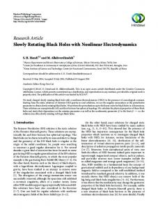
Here the parameter values c, η1 , η2 are included as additional unknowns and three phase conditions are added in order obtain a well-posed boundary value problem accessible to the package [5]. Real and imaginary parts of the solution are shown in Figure 1.
Figure 1: Real and imaginary part of spinning solitons in the QCGL-system. With the numerical solution at hand, the same code is used to compute a prescribed number neig of eigenvalues of the linearized finite element operator. The code uses the package ARPACK with a prescribed real shift σ ∈ R and is expected to give the neig eigenvalues closest to σ. We have B∞ = µI, which satisfies Assumption 2 since µ < 0. Assumptions 3 and 4 will be checked numerically. Our reference discretization uses the values R = 30, hmax = 0.25, neig = 400, σ = 3
(8.4)
which leads to a matrix eigenvalue problem with about 105 eigenvalues. The spectral picture corresponding to this choice is Figure 2 showing neig = 400 eigenvalues close to σ = 3. We observe a zig-zag type cluster of eigenvalues which one expects to correspond to essential spectrum. In fact, the structure will be explained by Theorem 8.1 below. In addition, the three eigenvalues ±ic and 0 on the imaginary axis are clearly visible in Figure 2. Moreover, Figure 2 suggests that there are eight additional complex conjugate pairs of eigenvalues lying between the imaginary axis and the zig-zag structure. For these eight pairs we have boxed the 8 eigenvalues with positive imaginary part. Note that one of the boxed eigenvalues near the top is rather close to the zig-zag structure, but does not belong to it. The 46
R=30, hmax=0.25, neig=400 6
4
2
0
−2
−4
−6 −4
−3
−2
−1
0
1
Figure 2: Spectrum of linearization about spinning soliton eigenvalues ±ic and 0 are also boxed. In addition, we have boxed two (numerical) eigenvalues appearing near the center at two tips of the zig-zag structure. Figure 3 plots the real parts of the eigenfunctions corresponding to the 12 boxed eigenvalues. Note that the eigenfunctions numbered 1 to 10 are localized; these eigenfunctions correspond to the eigenvalues 0 and ic as well as to the eight isolated eigenvalues not belonging to the zig-zag structure. The eigenfunctions numbered 11 and 12 correspond to the two boxed eigenvalues at the tips of the zig-zag stucture; as expected, these eigenfunctions are not localized since they correspond to essential spectrum. To validate our findings we have varied two parameters in the reference configuration (8.4): 1. Decrease radius to R = 20. The spectral picture is Figure 4 (left); the eigenfunctions are similar to those in Figure 3 (not shown). 2. Coarsen the grid to hmax = 0.5. The spectral picture is Figure 4 (right); the eigenfunctions are similar to those in Figure 3 (not shown). As already mentioned, the zig-zag structure in Figure 2 corresponds to essential spectrum of L. Therefore, our tests confirm that there are eight pairs of isolated eigenvalues between the essential spectrum and the imaginary axis. Since the corresponding eigenfunctions are localized and since there are no unstable eigenvalues, Assumptions 3 and 4 are confirmed. As one expects, variation of the size of the domain has a strong impact on the clusters that approximate the essential spectrum while refining the mesh does no change the clusters very much. On the other hand, looking at numerical values (not shown) one finds that convergence towards the isolated eigenvalues is best observed when the mesh-size is varied.
47
Figure 3: Eigenvalues and eigenvectors corresponding to boxes in Figure 2, the first two correspond to 0 and ic, the next eight to isolated and stable eigenvalues, the last two to spectral values at the tip of the zig-zag structure We refer to the work by Sandstede and Scheel [17],[14] on absolute spectra, which is relevant when studying perturbations such as truncation to a bounded domain. For the three eigenvalues ±ic and 0 on the imaginary axis we have also compared the numerical eigenfunctions ϕj,h with the eigenfunctions D1 u∗ ± iD2 u∗ and φ3 = Dφ u∗ given by Lemma 2.3. Here we have used the computed numerical approximation for u∗ (as a solution of (8.3)) and have evaluated its derivatives numerically. The resulting errors are
inf
θ∈[0,2π]
kϕ1,h − ϕ1 kL2
kϕ2 − eiθ (ϕ2,h + iϕ3,h )kL2
= 8.6510−3 = 4.3910−3 .
In view of the tolerances used, these results give satisfactory tests. Remark : We note that equation (8.1) happens to have an extra S 1 symmetry given by F (eiθ u) = eiθ F (u), 48
θ ∈ S 1,
(8.5)
R=30, hmax=0.5, neig=400
R=20, hmax=0.25, neig=400 6
10
4 5 2
0
0
−2 −5 −4
−10 −5
−4
−3
−2
−1
0
−6 −5
1
−4
−3
−2
−1
0
1
Figure 4: Spectrum of spinning soliton in the QCGL-system on a smaller ball (R = 20, left) and for a coarser grid (∆x = 0.5, right) where F denotes the right hand side of (8.1). Numerical computations suggest that the rotating wave u∗ satisfies u∗ (Rθ x) = eiθ u∗ (x). Then u∗ is also a relative equilibrium with respect to the group action of G = S 1 × R2 given by (cf. (1.11)) (a(η, θ)u) (x) = e−iθ u(x − η).
This leads to a simpler linearization where Dφ is not present and, therefore, a simpler stability analysis is possible than provided by our Theorem. However, this special situation can be easily avoided by destroying the symmetry (8.5) in (8.1). For example, we can perturb the complex factor γ in the two-dimensional real version of (8.1) so that it no longer corresponds to multiplication by a complex number. Numerical experiments show that the spinning solitons and the structure of the spectrum persist for the modified system.
8.2
On the Essential Spectrum of L
We use the following terminology ([11, Ch.5]): Definition 8.1. Let X denote a complex Banach space and let A : D(A) ⊂ X → X denote a closed, densely defined linear operator. A point λ ∈ C is in the resolvent set of A if A − λ : D(A) → X is 1–1, onto, and (A − λ)−1 is a bounded operator on X. An eigenvalue λ0 of A is called isolated if for some ε > 0 all λ with 0 < |λ0 − λ| < ε belong to the resolvent set of A. The multiplicity of the eigenvalue λ0 is the dimension of the algebraic eigenspace {u ∈ X : (A − λ0 )k u = 0 for some k ∈ N}. A point λ ∈ C is a normal point of A if either λ is in the resolvent set of A or λ is an isolate eigenvalue of A of finite multiplicity. All points of the complex plane which are not normal points form the essential spectrum of A, denote σess (A). Consider the linear operator L in (1.17) under the assumptions of Section 1. A part of the spectrum of L can be determined in terms of the constant matrices A and B∞ . To show this, we use polar coordinates and write 49
1 1 Lu = A(urr + ur + 2 uφφ ) + cuφ + (B∞ + Bδ (r, φ))u r r where Bδ = B − B∞ , thus (using Assumption 1), ηR := sup max |Bδ (r, φ)| → 0 as r≥R
R→∞.
φ
First neglect the O(1/r) terms and the term Bδ u in Lu and consider the simplified operator Lsim u = Aurr + cuφ + B∞ u . If u(r, φ) = einφ eiκr u ˆ with
n ∈ Z,
κ ∈ R,
u ˆ ∈ Cm ,
(8.6) |ˆ u| = 1 ,
(8.7)
then (Lsim − s)u = (−κ2 A + inc + B∞ − s)u .
Therefore, (Lsim − s)u = 0 if and only if
(−κ2 A + B∞ )ˆ u = (s − inc)ˆ u. This suggests the following: Theorem 8.1. For κ ∈ R let λj (κ) denote the eigenvalues of the matrix −κ2 A + B∞ for j = 1, . . . , m. Then the numbers s = inc + λj (κ),
n ∈ Z,
κ ∈ R,
j = 1, . . . , m ,
belong to the essential spectrum of L. Proof. In this proof we denote the L2 –norm on L2 (R2 , Cm ) by k · k. Assume that (−κ2 A + B∞ )ˆ u = λj (κ)ˆ u, |ˆ u| = 1, and let s = inc + λj (κ). For large real R choose C ∞ cut–off functions χR : [0, ∞) → [0, 1] with χR (r) = 1 χR (r) = 0
for R ≤ r ≤ 2R ,
for 0 ≤ r ≤ R − 1 or
and derivatives bounded independently of R. Set uR (r, φ) = χR (r)u(r, φ)
50
2R + 1 ≤ r < ∞
with u(r, φ) given in (8.6). Clearly, (Lsim − s)uR (r, φ) = 0 unless R−1≤r ≤R
or
2R ≤ r ≤ 2R + 1 .
(8.8)
Also, in the region (8.8), |(Lsim − s)uR (r, φ)| ≤ C with C independent of R. We have 2
kuR k ≥ 2π and
Z
2R
r dr = 3πR2
R
k(Lsim − s)uR k2 ≤ CR .
If we consider the operator L instead of Lsim , then (L − s)uR (r, φ) = 0
for r ≤ R − 1 and
r ≥ 2R + 1 .
Furthermore, |(L − s)uR (r, φ)| ≤ C
for
R−1≤r ≤R
and 2R ≤ r ≤ 2R + 1
and |(L − s)uR (r, φ)| ≤
C + ηR r
for
R ≤ r ≤ 2R .
Therefore, 2 k(L − s)uR k2 ≤ CR + CR2 ηR .
To summarize, the function uR ∈ L2 (R2 ) satisfies kuR k2 ≥ 3πR2
and
2 k(L − s)uR k2 ≤ CR + CR2 ηR .
If one sets vR = uR /kuR k then k(L − s)vR k2 ≤
C 2 + CηR →0 R
as
R→∞.
Therefore, either s is an eigenvalue of L or (L − s)−1 is unbounded on L2 . If s = inc + λj (κ) is an eigenvalue of L, varying κ shows that s cannot be isolated in the sense of Definition 1. Therefore, all numbers s = inc + λj (κ belong to the essential spectrum of L. 51
Illustration: The spectral values s of L determined by Theorem 8.1 form m sequences of lines, s = s(κ, n, j) = inc + λj (κ),
n ∈ Z,
κ ∈ R,
j = 1, . . . , m .
For illustration, consider the scalar case where A = a = a1 + ia2 is a complex number and B∞ = b∞ is a real number with a1 > 0 > b∞ . Then the values s determined by Theorem 8.1 are s = inc − κ2 (a1 + ia2 ) + b∞ ,
n ∈ Z,
κ∈R.
If a2 = 0 these are horizontal half–lines parallel to the subinterval (−∞, b∞ ] of the negative real axis. If a2 6= 0 the half-lines are tilted. Since the sequence of these half–lines belongs to the spectrum of L, the semi–group etL cannot be analytic. Application to QCGL: Proceeding as above, we find that the half–lines s = inc − κ2 α + µ
and s = inc − κ2 α ¯+µ ¯,
n ∈ N,
κ∈R,
belong to the essential spectrum of L. Since α = (1 + i)/2 is complex and µ ∈ R, µ < 0, the above lines form a zig-zag structure to the left of the imaginary axis; this agrees with the numerical findings of Section 8.1.
References [1] H. W. Alt, Lineare Funktionalanalysis (3rd ed.). Springer, 1999. [2] P. W. Bates and C. K. R. T. Jones, Invariant manifolds for semilinear partial differential equations. In Dynamics Reported Vol. 2, (U. Kirchgraber, H.O. Walther Eds.), 1-38, Teubner, 1989. [3] W.-J. Beyn and V. Th¨ ummler, Freezing solutions of equivariant evolution equations, SIAM Journal on Applied Dynamical Systems 3 (2004), 85-116. [4] P. Chossat and R. Lauterbach, Methods in equivariant bifurcations and dynamical systems. Advanced Series in Nonlinear Dynamics Vol. 15, World Scientific Publishing, 2000. [5] Comsol, Comsol Multiphysics 3.3, Comsol Inc., www.comsol.com, 2007. [6] L.-C. Crasovan, B. A. Malomed, and D. Mihalache, Stable vortex solitons in the twodimensional Ginzburg–Landau equation, Phys. Rev. E, 63 (2001), 016605. [7] L.-C. Crasovan, B. A. Malomed, and D. Mihalache, Spinning solitons in cubic-quintic nonlinear media, Pramana J. Phys., 57 (2001), pp. 1041–1059. 52
[8] K.-J. Engel and R. Nagel, One-Parameter Semigruops for Linear Evolution Equations. Graduate Texts in Mathematics, Springer, 2000. [9] A. Ghazaryan, Y. Latushkin, S. Schecter and A. J. De Souza, Stability of gasless combustion fronts in one-dimensional solids. Preprint, 2008. [10] I.C. Gohberg and M. G. Krˇein, Introduction to the Theory of Linear Nonselfadjoint Operators. Translations of Mathematical Monographs Vol. 18, American Mathematical Society, 1969. [11] D. Henry, Geometric Theory of Semilinear Parabolic Equations. Lecture Notes in Mathematics, Springer, 1981. [12] E. Hille and R. Phillips, Functional Analysis and Semi-Groups, AMS Colloquium Publications XXXI, 1957. [13] A. Pazy, Semigroups of linear operators and applications to partial differential equations (2.corr.print). Applied Mathematical Sciences Vol. 44, Springer, 1983. [14] J. Rademacher, B. Sandstede and A. Scheel, Computing absolute and essential spectra using continuation, Physica D 229, No. 2, 166-183, 2007., [15] M. Renardy and R.C. Rogers, An Introduction to Partial Differential Equations. Texts in Applied Mathematics Vol.13, Springer, 1993. [16] B. Sandstede, A. Scheel and C. Wulff, Dynamics of spiral waves on unbounded domains using center-manifold reductions. J. Differential Equations 141, 122-149, 1997. [17] B. Sandstede and A. Scheel, Absolute versus convective instability of spiral waves. Physical Review E, 62, No. 6, 7708-7714, 2000. [18] B. Sandstede, Stability of travelling waves. In Handbook of Dynamical Systems Vol. 2 (B. Fiedler Ed.), 983-1055, North-Holland, 2002. [19] A. E. Taylor and D. C. Lay Introduction to Functional Analysis (2nd ed). Wiley, 1980. [20] K. Yosida, Functional Analysis. Grundlehren der mathematischen Wissenschaften in Einzeldarstellungen 123 (4th ed.), Springer, 1974.
A
Perturbation Theorem for C0 -Semigroups
In this section X denotes a complex Banach space and A : D(A) ⊂ X → X is a densely defined linear operator generating the C0 –Semigroup etA . For the general theory we refer to [12], [13], [15], [8], see also Definition 8.1 for the notions of spectra used in this paper. It is known that etA may have continuous spectrum unrelated to the spectrum of A; see, for example, Theorem 16.7.4 of [12]. This raises the possibility of exponential growth of ketA k 53
even if the spectrum of A lies in the left–half plane. Theorem A.1, shown below, can be used to prove that exponential growths of ketL k does not occur for the operator L defined in (2.11). In fact, if we restrict etL to the space W = Ψ⊥ defined in (2.17), then ketL k decays exponentially. Recall that the (Liapunov) type of the C0 –semigroup etA is defined by ωA = lim
t→∞
log ||etA || log ||etA || = inf t>0 t t
(A.1)
and that, for any ω > ωA , there is an equivalent norm || · ||ω (see [15, Th.11.21]) with ||etA ||ω ≤ etω ,
t ≥ 0.
(A.2)
In our main result we estimate the type number of a perturbed semigroup, et(A+B) , in terms of the type number ωA of A and a bound ω+ on the real parts of the eigenvalues of A + B: Theorem A.1. Let A : D(A) ⊂ X → X denote the generator of a C0 -semigroup of type ωA . Further, assume that B ∈ L[X] is a linear bounded operator so that BetA
is compact for all
t > 0.
(A.3)
Then A + B : D(A) → X generates a C0 -semigroup on X that satisfies |σess (eA+B )| ≤ eωA . If, in addition, Re λ ≤ ω+
then the semigroup
et(A+B)
for all eigenvalues
(A.4)
λ∈C
of
A + B,
(A.5)
is of type ωA+B where ωA+B ≤ max(ωA , ω+ ).
(A.6)
The proof of Theorem A.1 uses two auxiliary results. Lemma A.1. Let exp(tA) be a C0 -semigroup on X and let M ⊂ X be precompact. Then sup ||(exp(tA) − I)u|| → 0
u∈M
as t → 0
(A.7)
Proof. Suppose, to the contrary, that for some δ > 0 we can find sequences un ∈ M, tn → 0 such that ||(exp(tn A) − I)un || ≥ δ for all n ∈ N.
W.l.o.g assume limn→∞ un = u ˆ ∈ X and choose tˆ > 0 such that ||(exp(tA) − I)ˆ u|| ≤ ˆ 0 < t ≤ t. Then we obtain for n large ||(exp(tn A) − I)un || ≤ || exp(tn A)(un − u ˆ)|| + ||(exp(tn A) − I)ˆ u|| ≤ a contradiction.
+ ||ˆ u − un || � δ δ ˆ|| + ≤ , Ceωtn + 1 ||un − u 4 2 54
δ 4
for
For the following perturbation result see [10, Ch.1],[11, Ch.5]. Theorem A.2. Let T : D(T ) ⊂ X → X denote a closed linear operator and let S : D(S) ⊂ X → X be a linear operator such that D(T ) ⊂ D(S) and S(λ0 − T )−1 is compact for some λ0 ∈ C. Let Ω ⊂ C be open connected and contain only normal points of T . Then either Ω consists entirely of normal points of T + S or entirely of eigenvalues of T + S. Proof. (Theorem A.1) Let ω > ωA be given and, as in (A.2), select a norm || · ||∗ such that 1 || exp(tA)||∗ ≤ exp( (ωA + ω)t), 2
t ≥ 0.
(A.8)
It is well known that A + B is the generator of a C0 -semigroup that is of type ωA+B ≤ ωA + ||B||∗ (cf. [15, Ch.11.2]). In particular, it follows from (A.8) that � � ωA + ω ) ≤ exp (t(||B||∗ + ω)) , t ≥ 0. (A.9) || exp(t(A + B))||∗ ≤ exp t(||B||∗ + 2 It remains to prove (A.6). By the variation of constants formula 5 we have for each u ∈ X Z t exp((t − s)(A + B))B exp(sA)uds. (A.10) exp(t(A + B))u = exp(tA)u + 0
We multiply by
e−ωt
and evaluate at t = 1 to obtain
exp(A − ω + B)u = exp(A − ω)u + Ku Z 1 Ku = exp((1 − s)(A − ω + B))B exp(s(A − ω))uds.
(A.11) (A.12)
0
Note that by (A.8)
1 (A.13) || exp(A − ω)||∗ ≤ exp(− (ω − ωA )) =: q < 1. 2 We show that for each ε > 0 there exists a compact operator Kε such that ||K − Kε ||∗ ≤ ε. Then the operator K defined in (A.12) is a uniform limit of compact operators and hence compact itself. First, we rewrite (A.12) for 0 < t0 ≤ 1 Ku = K0 u + K1 u Z t0 exp((1 − s)(A − ω + B))B exp(s(A − ω))uds = 0 Z 1 + exp((1 − s)(A − ω + B))B0 exp((s − t0 )(A − ω))uds,
(A.14)
t0
5 If at = Aa, bt = (A + B)b, a(0) = b(0) = u, then (b − a)t = (A + B)(b − a) + Ba and b(t) = a(t) + R t (t−s)(A+B) e Ba(s) ds, yielding (A.10). 0
55
where B0 = B exp(t0 (A − ω)).
(A.15)
Here we choose t0 so small that for all u ∈ X: Z t0 s ε exp((1 − s)||B||∗ )||B||∗ exp(− (ω − ωA ))ds||u||∗ ≤ ||u||∗ . ||K0 u||∗ ≤ C 2 2 0
(A.16)
0 We approximate the integral in K1 by step functions on the grid tj = t0 + j 1−t N , j = 0, . . . , N
K1 u =
N −1 Z tj+1 X j=0
=
N −1 Z X j=1
=
N −1 X j=0
+
tj
N −1 X j=0
1−t0 N
0
· · · ds exp((1 − (tj + τ ))(A − ω + B))B0 exp((tj + τ − t0 )(A − ω))udτ
exp((1 − tj+1 )(A − ω + B))B0
Z
1−t0 N
exp((τ + j
0
1 − t0 )(A − ω))udτ N
exp((1 − tj+1 )(A − ω + B))
1−t0 N
1 − t0 1 − t0 − τ )(A − ω + B)) − I)B0 exp((τ + j )(A − ω))udτ N N 0 = KN u + RN u. Z
(exp((
By our assumption the operator B0 in (A.15) is compact, hence KN is compact and can be taken as approximation of K. Compactness of K follows if we show that ||RN ||∗ → 0 as N → ∞. 0 For ||u||∗ ≤ 1 and j = 0, . . . , N − 1, 0 ≤ τ ≤ 1−t N we have by (A.13) || exp((
j (1 − t0 ) + τ )(A − ω))u||∗ ≤ 1. N
(A.17)
Now apply Lemma A.1 to the precompact set M0 = {B0 u : ||u||∗ ≤ 1} and obtain δ = δ(ε) > 0 so that for 0 ≤ s ≤ δ: sup ||(exp(s(A − ω + B)) − I)v||∗ ≤
v∈M0
Using (A.8) we then have the following estimate for N ≥ ||RN ||∗ ≤
ε||B||∗ . 2(e||B||∗ − 1) 1 δ
N −1 X ε||B||∗ ε e(1−tj+1 )||B||∗ ≤ . ||B||∗ 2 2N (e − 1) j=0
This completes the proof of the compactness of K. 56
(A.18)
(A.19)
In the next step we apply Theorem A.2 with the settings T = exp(A − ω), S = K, λ0 = 1, and Ω = {λ ∈ C : |λ| > q}. By (A.13) the operator (T − 1)−1 exists and is continuous, hence K(T − 1)−1 is compact. Since exp(A − ω + B) is bounded, the set Ω has points in the resolvent and thus |σess (exp(A − ω + B))| ≤ q. (A.20) We have shown 1 |σess (exp(A + B))| ≤ qeω = exp( (ω + ωA )) 2
for all
ω > ωA ,
which proves our first assertion (A.4). Now consider ω > max(ωA , ω+ ). For the point spectra we conclude from [13, Theorem 2.4] σpoint (exp(A − ω + B)) ⊂ exp(σpoint (A − ω + B)) ∪ {0}.
(A.21)
(Note that in reference [13] the set σpoint contains, by definition, all eigenvalues, not necessarily isolated or of finite multiplicity.) By assumption (A.5) we have Re σpoint (A+B−ω) ≤ ω+ −ω < 0 which leads to |σpoint (exp(A−ω+B))| ≤ eω+ −ω . Combining this with (A.20) yields the estimate for the whole spectrum |σ(exp(A − ω + B))| ≤ max(q, eω+ −ω ) < 1.
(A.22)
Therefore, we can construct a new equivalent norm || · ||+ such that || exp(A − ω + B)||+ ≤ 1.
(A.23)
This implies || exp(n(A − ω + B))||+ ≤ 1 for all n ∈ N and, by filling the finite gaps with the help of (A.9), || exp(t(A − ω + B))||+ ≤ C = max || exp(s(A − ω + B))||+ , 0≤s≤1
t ≥ 0.
(A.24)
This shows that the semigroup has type at most ω. Since the choice of ω > max(ωA , ω+ ) was arbitrary, the proof is complete.
57


![arXiv:1112.5087v1 [math.PR] 21 Dec 2011 - SFB 701 - Universität ...](https://m.moam.info/img/260x300/arxiv11125087v1-mathpr-21-dec-2011-sfb-701-univers_5ba9f989097c47e73e8b474b.jpg)
![arXiv:1501.01198v1 [math.DS] 6 Jan 2015 - SFB 701 - Universität](https://m.moam.info/img/260x300/arxiv150101198v1-mathds-6-jan-2015-sfb-701-univers_5c9f6a03097c4757428b46db.jpg)
![arXiv:1605.08635v1 [math.PR] 27 May 2016 - SFB 701](https://m.moam.info/img/260x300/arxiv160508635v1-mathpr-27-may-2016-sfb-701_5c1aaa12097c47c0738b4607.jpg)