Nonparametric Cusum Charts for Angular Data with Applications in ...

arXiv:1705.00351v1 [stat.ME] 30 Apr 2017

Nonparametric Cusum Charts for Angular Data with Applications in Health Science and Astrophysics F. Lombard Center for Business Mathematics and informatics North-West University, Potchefstroom, South Africa Douglas M. Hawkins Scottsdale Scientific LLC, Scottsdale, AZ Cornelis Potgieter Department of Statistical Science Southern Methodist University, Dallas, TX Abstract This paper develops non-parametric rotation invariant CUSUMs suited to the detection of changes in the mean direction as well as changes in the concentration parameter of angular data. The properties of the CUSUMs are illustrated by theoretical calculations, Monte Carlo simulation and application to sequentially observed angular data from health science and astrophysics. Key words: Angular data, Cusum, Nonparametric

1

1

Introduction

Sequential CUSUM methods for detecting parameter changes in distributions on the real line is a well developed field with an extensive literature. The same cannot be said about CUSUM methods in non-Euclidean spaces such as the circle. Distributions on the circle generate angular data which, for obvious reasons, cannot be treated in the same manner as linear data. Lombard, Hawkins and Potgieter (2017) reviewed the current state of change detection procedures for angular data. They also constructed distributionfree CUSUMs for angular data in which the numerical value of an in-control mean direction is specified, the objective being to detect a change in mean direction away from this value. The situation is analogous to that of detecting a change away from a specified numerical value of the mean of a distribution on the real line. In some situations, such as those treated in Section 4 of the present paper, no in-control parameter value is specified and the objective is to detect a change in the mean away from the current value, whatever it may be. Hawkins (1987) constructed a self starting CUSUM that is capable of detecting efficiently changes away from a current, unknown, mean of a normal distribution when the variance is also unknown. In the present paper, we construct CUSUMs for angular data in the same spirit, except that no assumption of a specific parametric distribution specification is made. In this sense, our CUSUMs are nonparametric. They are not, however, fully distribution-free but are shown in a Monte Carlo study to be nearly so over a wide class of angular distributions. We develop CUSUMs to detect changes in mean direction as well as in concentration. Section 2 of the paper focuses on mean direction. We provide parametric and nonparametric justifications for our CUSUM and elaborate on its incontrol and out-of control properties. The results of an extensive Monte Carlo study are also reported. In Section 3 we consider concentration changes. Section 4 demonstrates the application of the CUSUMs to two sets of real data and Section 5 summarizes our results.

2

2 2.1

Detecting direction change Derivation of the CUSUM statistic

Initially the data X1 , X2 , . . . come from a non-uniform continuous distribution F with unknown mean direction ν = ν0 on the circle [−π, π). This defines the in-control state. (Since mean direction is a vacuous concept in a uniform distribution, the latter is excluded from consideration. The CUSUM of Lombard and Maxwell (2012) can be used to detect a change from a uniform to a non-uniform distribution.) We estimate ν by νˆn = atan2(Sn , Cn ) where for n = 2, 3, . . ., Cn =

Pn

j=1 cos

X j , Sn =

Pn

j=1 sin

Xj ,

and atan2 denotes the four-quadrant inverse tangent function  tan−1 (x/y) if y > 0    −1 tan (x/y) + πsign(x) if y < 0 atan2(x, y) = (π/2)sign(x) if y = 0, x 6= 0    0 if y = x = 0

(1)

,

the symbol tan−1 denoting the usual inverse tangent function with range restricted to (−π/2, π/2). This non-parametric estimator is, in fact, also the maximum likelihood estimator of mean direction in a von Mises distribution, which is arguably the best known among angular distributions. The von Mises distribution with mean direction ν and concentration κ, has density function f (x) =

1 exp(κcos(x − ν)), 2πI0 (κ)

−π ≤ x < π, where I0 denotes the modified Bessel function of the first kind of order zero. The log-likelihood ratio based on observations X1 + δ, . . . , Xn + δ is, apart from a factor not depending upon δ, given by l(δ) = cos(Xn − δ − ν)

3

and a locally most powerful test of the hypothesis H0 : δ = 0 is therefore based on the derivative  dl(δ) = sin(Xn − ν). dδ δ=0 Replacing ν by νˆn−1 leads to consideration of a CUSUM based on the statistic Vn = sin(Xn − νˆn−1 ).

(2)

Despite the fact that Vn originates from the von Mises distribution, it also has at least two purely non-parametric origins that do not depend upon any assumption involving the type of the underlying distribution. The first of these follows upon expanding the sine function and using the trigonometric relations sin(ˆ νn−1 ) = Sn−1 /Rn−1 ; cos(ˆ νn−1 ) = Cn−1 /Rn−1 , wherein Rn2 = Cn2 + Sn2 .

(3)

Vn = (Cn−1 /Rn−1 )sin Xn − (Sn−1 /Rn−1 )cos Xn ,

(4)

This gives

which is the (signed) area of the parallelogram spanned by the unit length vectors (Cn−1 , Sn−1 )/Rn and (sin Xn , cos Xn ). The former of these vectors points in the mean direction of the data X1 , . . . , Xn−1 while the latter vector points in the direction of the new observation Xn . Thus, if a change in mean direction ν occurs at index n, we can expect a succession of large positive or large negative values Vn , n > τ . A second non-parametric argument leading to consideration of Vn comes from considering the change νˆn − νˆn−1 in the estimate of ν effected by a change in mean direction from ν to ν + δ occurring at index n. We have νˆn = atan2(Sn−1 + sin (Xn + δ), Cn−1 + cos (Xn + δ)) = atan2(Sn−1 /n + δ1,n , Cn−1 /n + δ2,n )

4

where nδ1,n = sin (Xn + δ) = sin Xn + O(δ), nδ2,n = cos (Xn + δ) = cos Xn + O(δ). Since both Sn−1 /n and Cn−1 /n converge as n → ∞ and both δ1,n and δ2,n tend to zero, we can make a Taylor expansion around (Sn−1 /n, Cn−1 /n). This gives Rn−1 (ˆ νn − νˆn−1 ) = nδ1,n =

Cn−1 Sn−1 1 − nδ2,n + O( ) Rn−1 Rn−1 n

Cn−1 Sn−1 1 sin Xn − cos Xn + O(δ) + O( ) Rn−1 Rn−1 n

1 = Vn + O(δ) + O( ), n which shows again the relevance of Vn for detecting changes in mean direction. The most important property of Vn as far as motivation for the present paper is concerned is its rotation invariance: its numerical values are unaffected if all the data are rotated through the same fixed, but unknown, angle. Thus, a CUSUM based on Vn will be applicable in situations where no in-control direction is specified and the objective is merely to detect deviations from this arbitrary in-control direction. Both examples treated in Section 4 of the paper are of this nature. This contrasts with the distributionfree CUSUMs in Lombard, Hawkins and Potgieter (2017), which require a specified numerical value of the in-control mean direction.

2.2

Construction of the CUSUM

When the process is in control, that is, when X1 , X2 , . . . are independently and identically distributed (but with unknown mean direction), then p ξn := (Vn − En−1 [Vn ])/ varn−1 [Vn ], n ≥ 2, (5)

is a martingale difference sequence with conditional variance 1. Here and elsewhere, En−1 [·] and varn−1 [·] denote expected value and variance computed conditionally upon X1 , . . . , Xn−1 . Using standard martingale central 5

limit theory, we can show that cumulative sums of the ξn will be asymptotically normally distributed regardless of the type of underlying distribution - see, e.g. Helland (1982, Theorem 3.2). Furthermore, if ν = ν0 changes by an amount δ to ν = ν0 + δ at observation Xτ +1 (τ being the last in-control observation) then by either of the two arguments following (2), we can expect Eτ [ξτ +1 ] to be non-zero. Thus, a standard two-sided normal CUSUM for data on the real line, applied to the ξn sequence, could be expected to be effective in detecting a change away from the initial direction. Furthermore, the in-control behaviour should be quantitatively similar to that of a standard normal CUSUM. The conditional mean and variance in (5) depend on the first two moments of sin X and cos X, which are unknown parameters. Accordingly, given observations X1 , . . . , Xn , we estimate the conditional mean and variance nonparametrically by 1 Xn−1 Eˆn−1 [Vn ] = sin(Xi − νˆn−1 ) = 0 i=1 n−1 and 1 Xn−1 2 vd arn−1 [Vn ] = sin2 (Xi − νˆn−1 ) := Bn−1 . i=1 n−1 Then a computable CUSUM is obtained upon replacing ξn in (5) by ξˆn = Vn /Bn−1 .

(6)

The CUSUM is started at observation m + 1 by setting Di± = 0 for i = 1, . . . , m and + Dm+n = max{Dm+n−1 + ξˆm+n − ζ}

(7)

− Dm+n = min{Dm+n−1 + ξˆm+n + ζ}

for n ≥ 1, where ζ is the reference value. The run length, N, is the first index + − n at which either Dm+n ≥ h or Dm+n ≤ −h, where h is a control limit. The control limit is chosen to produce a specified in-control average run length (ARL), which we denote throughout by ARL0 . The first m observations serve to make an initial estimate of the population moments after which the estimates are updated with the arrival of each new observation. Since the the random variables sin X and cos X are bounded, convergence of sample moments to population moments would be quite rapid so that a relatively small number m of observations should suffice to initialize the CUSUM. 6

2.3

Implementation

Implementation of the CUSUM scheme requires an efficient method of updating the summand ξˆn−1 upon arrival of a new observation Xn . For this, set sn = sin Xn ; cn = cos Xn and Cn(2) =

Pn

2 j=1 cj ,

Sn(2) =

and observe the simple recursions

Pn

2 j=1 sj ,

A(2) n =

Pn

j=1 sj cj .

Sn−1 = Sn−2 + sn−1 ; Cn−1 = Cn−2 + cn−1 , (2)

(2)

(2)

(2)

Sn−1 = Sn−2 + s2n−1 ; Cn−1 = Cn−2 + c2n−1 and

(2)

(2)

An−1 = An−2 + sn−1 cn−1 . To compute Vn , given Sn−2 , Cn−2, cn−1 , cn , sn−1 and sn , use the expression in (4) together with the first of these recursions. To compute Bn−1 , given (2) (2) (2) Sn−1 , Cn−1 , Sn−1, Cn−1 , An−1 , cn−1 , and sn−1 , observe that 2 (n − 1)Bn−1 =

2 2 Sn−1 Cn−1 Cn−1Sn−1 (2) (2) (2) S + Cn−1 − 2 An−1 . n−1 2 2 2 Rn−1 Rn−1 Rn−1

A rational basis for specifying a reference value ζ is also required. This aspect of the CUSUM design is considered in Section 2.5 of the paper.

2.4

In-control properties

While the proposed CUSUM is not distribution-free, the asymptotic incontrol normality of CUSUMs of ξˆn suggests that it may be nearly so. Then, use of standard normal distribution CUSUM control limits should lead to an in-control ARL sufficiently close to the nominal value to make the CUSUMs of practical use. (The requisite control limit h can be obtained from the widely available software packages of Hawkins, Olwell and Wang, (2016) or Knoth (2016)). To check this expectation we estimated by Monte Carlo simulation the in-control ARL over a range of unimodal symmetric and asymmetric distributions on the circle. Among the multitude of possible distributions, the class of wrapped stable and Student t distributions, together with their 7

skew versions, represent a wide range of unimodal distribution shapes on the circle. Simulated data from these distributions are easily obtained by generating random numbers Y from the distribution on the real line and then wrapping these around the circle by the simple transformation Y (mod 2π). Algorithms for generating the random numbers Y are given in Nolan (2015) and in Azzalini and Capitanio (2003). The algorithms were implemented in Matlab and the relevant programs are included in the supplementary material to this paper. Some simulations were also run on data from other types of distribution which are defined directly on the circle and not obtained by wrapping. Specifically, we used the sine-skewed distributions developed Umbach and Jammalamadaka (2011) and by Abe and Pewsey (2011). In contrast to the wrapped stable and Student t distributions, the densities of these distributions have closed form expressions, which facilitates model fitting and parameter estimation. However, the various unimodal distribution shapes available in these classes of distributions are quite similar to those in the class of wrapped distributions. Since the behaviour of a nonparametric CUSUM depends more on the general shape of the underlying distribution than on the specific parameter values producing that shape, it comes as no surprise that the in-control behaviour of the CUSUMs proposed here is quite similar in the two classes (wrapped and directly constructed) of distributions. Since wrapped distributions are widely known and understood, we frame our discussion in the context of these distributions. Some simulation results for data from the sine-skewed distributions are included in the supplementary material to this paper. In the discussion that follows, Sα , 0 < α ≤ 2, denotes a stable distribution with index α and tn , n ≥ 1 denotes a Student t-distribution with n degrees of freedom. In assessing the performance of the direction CUSUM under various symmetric in-control and out-of-control distributions, it seems sensible to standardize the observations to a common measure of concentration. The concentration parameter κ of the von Mises(ν, κ) distribution satisfies the relation κ = A−1 (E[cos(X − ν)])

(8)

where A(κ) = I1 (κ)/I0 (κ) and I1 denotes the modified Bessel function of the first kind of order 1. In view of the status of the von Mises distribution among circular distributions, which is much like that of the normal distribution among distributions on the real line, we use in this paper κ in (8) as a 8

measure of the concentration of a unimodal angular distribution with mean direction ν. Thus, given κ and the density function of Y , the scale parameter σ is chosen to make the distribution of the wrapped random variable X = (σY )w := σY (mod 2π) satisfy (8). For instance, suppose Y has an Sα distribution with characteristic function φ(t; α) = E[cos tY ] = exp(−|t|α ). Then (Jammallamadaka and SenGupta, 2001, Proposition 2.1), E[cos (σY )w ] = φ(σ; α) = exp(−σ α ) so that σ = (−log( A(κ)))1/α .

(9)

As another example, a Student t-distribution with α degrees of freedom has characteristic function √ √ Kα/2 ( αt)( αt)α/2 φ(t; α) = 2α/2−1 Γ( α2 ) where Kα/2 denotes the modified Bessel function of the second kind order α/2 and Γ denotes the gamma function. Thus, in this case, √ √ Kα/2 ( ασ)( ασ)α/2 E[cos (σY )w ] = φ(σ; α) = 2α/2−1 Γ( α2 ) , and σ is the solution to the equation √ √ α Kα/2 ( ασ)( ασ)α/2 = 2α/2−1 Γ( )A(κ). (10) 2 Some numerical values that were used in the simulation study which is reported next, are shown in Table 1. Table 1 Scale parameter σ solving (9) and (10) κ=1 κ=2 κ=3 S2 0.90 0.60 0.46 S1 0.81 0.36 0.21 S1/2 0.65 0.13 0.04 t3 1.07 0.64 0.46 t2 1.00 0.55 0.38 9

We used standard normal control limits in 50, 000 Monte Carlo realizations of the two-sided CUSUM in each of five underlying symmetric unimodal distributions: wrapped Student t-distributions with 2 and 3 degrees of freedom and three wrapped stable distributions with indexes α = 2 (the wrapped normal distribution), α = 1 (the wrapped Cauchy distribution, which is also the wrapped Student t-distribution with 1 degree of freedom) and α = 1/2 (the wrapped symmetrized L´evy distribution). Except for the wrapped normal, these are wrapped versions of heavy-tailed symmetric distributions on the real line. Each of the distributions was standardized to concentrations of κ = 1, 2 and 3 by specifying the scale parameter σ (see Table 1) in accordance with (9) and (10). Two sets of simulations were run. In the first set, the CUSUMs were initiated at n = 11, the first m = 10 observations serving to establish initial estimates of the unknown parameters. In the second set we took m = 25, initiating the CUSUM at n = 26. We present in Tables 2.1 and 2.2 aggregated sets of results representing the general picture. (Detailed tables are given in the supplementary material to this paper.) Each entry is the average of five estimated in-control ARLs, one from each of the five distributions. The number in brackets shows the range of the five estimates. The tables show the results for reference values ζ = 0 and ζ = 0.25. Table 2.1 In-control ARL of the non-parametric CUSUM in five symmetric distributions (m = 10) ζ =0 ζ = 0.25 ARL0 κ=1 κ=2 κ=3 κ=1 κ=2 κ=3 ∗ ∗ 250 242 (2) 243 (5) 242 (4) 236 (4) 233 (2) 225∗ (20) 500 490 (3) 491 (6) 491 (10) 493 (9) 483 (8) 464∗ (52) 1, 000 1037 (9) 1039 (14) 1042 (20) 1018 (7) 997 (30) 958∗† (117)

10

Table 2.2 In-control ARL of the non-parametric CUSUM in five symmetric distributions (m = 25) ζ=0 ζ = 0.25 ARL0 κ=1 κ=2 κ=3 κ=1 κ=2 250 244 (2) 244 (6) 245 (7) 242 (4) 239 (3) 500 492 (4) 493 (7) 493 (10) 498 (9) 491 (7) 1, 000 1039 (11) 1041 (10) 1045 (17) 1024 (13) 1005 (26)

κ=3 234∗ (8) 478 (28) 971 (82)

All but the four starred estimates shown in the Tables lie within 5% of the nominal value. The exceptions, which all lie within 10%, occur at ζ = 0.25 and predominantly at the smaller warmup m = 10. In the cell marked ∗† the five estimates were 874, 959, 976, 988 and 991, the outlier 874 coming from the very heavy-tailed L´evy distribution. In fact, all three discrepancies in this column are attributable to a substantial underestimate from the L´evy distribution Overall, the discrepancies between estimated in-control ARL values and nominal values are sufficiently small to inspire confidence in the use of the CUSUM with m ≥ 25 in practical applications. To assess the effect of skewness in the underlying distribution on the in-control ARL, we generated data from wrapped skew-normal distributions (Pewsey, 2000) with mean direction zero and skewness parameters λ = 2 (lightly skewed), λ = 7 (moderately skewed) and λ = ∞ (heavily skewed), wrapped skew-stable Cauchy- and L´evy distributions with skewness parameters β = 0.75 and 1.0 (Jammallamadaka and SenGupta, 2001, Section 2.2.8) and from wrapping skew-t distributions (Jones and Faddy, 2003) with 2 and 3 degrees of freedom and skewness parameters λ = 2, 7 and ∞ . The aggregated results are in Tables 3.1 and 3.2. Comparing the results with those in Tables 2.1 and 2.2, we see that the general pattern is the same. The main contributors to the apparent degradation seen at ζ = 0.25, κ = 3 are the excessively skewed distributions, namely the wrapped skew-normal and t-distributions with skewness parameter λ = ∞ and the wrapped L´evy distribution with skewness parameter β = 1. These distributions produce estimates that are consistently substantially lower than the rest. This is perhaps not too surprising if one takes account of their shape. At κ = 3 these densities are effectively concentrated on the semi-circle [0, π] .The supplementary material to this paper has a Figure showing a plot of a wrapped skew-t density with 2 degrees of freedom and skewness parameters λ = 0, 2 and 7 at κ = 3. It is apparent that the effect is already present to a large extent at 11

λ = 7. The implication is that a real line CUSUM should rather be applied to such data. The degradation noted above largely disappears when such excessively skew distributions are eliminated from consideration Table 3.1 In-control ARL of the non-parametric CUSUM in thirteen asymmetric distributions (m = 10) ζ =0 ζ = 0.25 ARL0 κ=1 κ=2 κ=3 κ=1 κ=2 κ=3 250 241 (2) 240 (4) 238 (7) 235 (5) 228 (11) 217 (25) 500 489 (4) 487 (6) 484 (9) 490 (8) 474 (29) 448 (71) 1, 000 1039 (11) 1036 (9) 1031 (13) 1013 (13) 979 (61) 915 (178) Table 3.2 In-control ARL of the non-parametric CUSUM in thirteen asymmetric distributions (m = 25) ζ=0 ζ = 0.25 ARL0 κ=1 κ=2 κ=3 κ=1 κ=2 κ=3 250 243 (2) 242 (3) 242 (4) 240 (3) 235 (7) 229 (22) 500 491 (5) 490 (6) 489 (7) 494 (7) 484 (25) 463 (59) 1, 000 1039 (13) 1038 (10) 1038 (11) 1019 (17) 988 (65) 935 (161)

2.5

Out-of-control properties

While the in-control behaviour of the CUSUM is similar to that of a CUSUM for normal data on the real line, the same is not true in respect of its outof control behaviour. In fact, from (6) we show next that a consequence of the continual updating of the mean direction estimator νˆn is that after a change of mean direction the CUSUM will return eventually to what appears to be an in-control state. This behaviour is similar to that of self-starting CUSUMs, and is a warning to users of the need for corrective action as soon as a change is diagnosed.- see Hawkins (1987) and Hawkins and Olwell (1997, Section 7.1). Suppose there is a rotation of size δ from n = τ + 1 onwards and set Yi = Xi+τ + δ, i ≥ 1 Then, using the approximations k 1 ≈ 0 and ≈1 τ +k τ +k 12

for large k and fixed τ ≥ m, the mean direction estimated from the data X1 , . . . , Xτ , Y1 , . . . , Yk is ! P P Sτ + ki=1 sin Yi Cτ + ki=1 cos Yi νˆτ +k = atan2 , τ +k τ +k

≈ atan2

Pk

i=1 sin Yi , k

Pk

i=1 cos Yi k

!

:= νˆk (Y ),

which is the estimated mean direction of Yi , 1 ≤ i ≤ k. Thus, for sufficiently large k, νˆτ +k is in effect estimating the mean direction of the post-change observations Y1 , . . . , Yk . Consequently, sin(Yk+1 − νˆk (Y )) ξˆτ +k+1 ≈ q P k 1 2 ˆk (Y )) i=1 sin (Yi − ν k

which, because of its rotation invariance, has the same distribution as the in-control variable ξˆk . A further consequence of this behaviour is that there is no simple manner in which to assess, a priori, the out-of-control ARL E[N − τ |N > τ ] of the CUSUM. Here N − τ is the time taken for an alarm to be raised after a change has occurred, the expected value being calculated upon an assumption of no false alarms prior to the change. Nevertheless, simulation results indicate that the out-of-control ARL of the two-sided CUSUM behaves in an appropriate manner, namely that the out-of-control ARL is less than the in-control ARL0 and that it decreases as the size of the shift increases from 0 to π/2. For shifts of size in excess of π/2,the ARL starts to increase again. This behaviour is a result of the periodic nature of the CUSUM summand. To illustrate the general pattern of out–of-control ARL behaviour, Table 4 gives out–of-control ARL estimates from simulations involving shifts of sizes ranging from π/8, to 7π/8 in a wrapped Cauchy distribution with κ = 2, a warmup sample size m = 25 and reference constants ζ = 0 and ζ = 0.25. The in-control ARL was 1000 throughout. The results are for shifts induced at observation τ = 100 and observation τ = 200. 13

Table 4

Estimated out–of-control ARL of direction CUSUM. m = 50, τ = m + 50 = 100 and τ = m + 150 = 200 τ = 100 τ = 200 ζ = 0 ζ = 0.25 ζ = 0 ζ = 0.25 δ = π/8 123 82 82 39 δ = π/4 50 14 40 13 δ = π/2 31 8 28 8 δ = 3π/4 38 12 37 12 δ = 7π/8 58 26 61 28

In our applications in Section 4, the objective is to detect change of any extent. No specific out-of-control change size δ0 is targeted in the sense that changes of size less than δ0 are thought to be inconsequential. However, should such a target be specified, it is not at all clear what would be an appropriate reference value ζ. If τ denotes the changepoint, define Vτ +1 (δ) = sin(Xτ +1 + δ − νˆτ ). Then, a Taylor expansion around δ = 0 gives Vτ +1 (δ) = Vτ +1 + δcos(Xτ +1 − νˆτ ) + O(δ 2) with Vτ +1 := Vτ +1 (0) given in (2). Consequently, ˆτ [Vτ +1 ] + δ Eˆτ [cos(Xτ +1 − νˆτ )] + O(δ 2 ) Eˆτ [Vτ +1 (δ)] = E =δ×

1 Xτ cos(Xj − νˆτ ) + O(δ 2). j=1 τ

In analogy with a normal distribution CUSUM, an appropriate choice of reference constant based on in-control Phase I data X1 , . . . , Xm and a target δ0 could then be Pm 1 ˆm ) δ j=1 cos(Xj − ν 0 m ζˆ = (11) ×q P m 2 1 2 ˆm ) j=1 sin (Xj − ν m .

Of course, the effect of any such Phase I estimation on the in-control Phase ˆ let h ˆ be the II performance of the CUSUM needs to be considered. Given ζ, 14

control limit which gives a standard normal CUSUM an in-control ARL value ARL0 . The simulation results in Section 2.4- see Tables 2 and 3 - indicate that the resulting Phase II CUSUM is near distribution-free. Thus, regardless of the form of the underlying distribution, the true Phase II in-control ARL will be nearly constant and acceptably close to the nominal value ARL0 . This behaviour is in stark contrast to that of parametric CUSUMs where estimating unknown parameters from Phase I data and then pretending that the Phase I estimate is the true value, affects irrevocably the in-control ARL of the Phase II CUSUM. In such cases there is no guarantee that the incontrol ARL will be equal to, or even near, the nominal value. This point has been made repeatedly in the published literature, most recently by Keefe, et al. (2015). Hawkins and Olwell (1997, pages 159-160) give a realistic example in which the true in-control ARL of a normal distribution CUSUM, with variance estimated from Phase I data, differs by two orders of magnitude from the nominal value.

3

Detecting a change in concentration

For data X1 , . . . , Xn from a von Mises(ν, κ) distribution, locallyP most powerful tests of the hypothesis κ = κ0 (6= 0) are based on the statistic ni=1 cos(Xi − ν). However, the fact that κ is not a scale parameter of the distribution of X complicates matters. Hawkins and Lombard (2017) showed that even if the mean direction ν is known, control limits for a specified in-control ARL in a von Mises CUSUM for detecting change away from κ0 depend upon κ0 . Nonetheless, the locally most powerful test statistic suggests application of a CUSUM based on Vn′ = cos(Xn − νˆn−1 ), n ≥ 1. Again, there are purely non-parametric interpretations of Vn′ , devoid of any reference to a von Mises distribution. For instance, since Vn′ = (Cn−1 /Rn−1 )cos Xn + (Sn−1 /Rn−1 )sin Xn , we see that Vn′ is the (signed) length of the projection of the vector yn = (sin Xn , cos Xn ) in the direction νˆn−1 ≈ ν of the unit vector (Sn−1 /Rn−1 , Cn−1 /Rn−1 ). If the concentration increases (decreases) after n = τ , the average of Vτ′+1 , . . . , Vτ′+k will tend to be greater (smaller) than 15

the average of V1′ , . . . , Vτ′ . Another non-parametric interpretation rests on the fact that Rn2 in (3) is a frequently used non-parametric measure of concentration in a sample X1 , . . . , Xn . Simple algebra shows that the relative 2 change in Rn−1 brought about by the next observation Xn is Rn2 2Vn′ 1 − 1 = + 2 2 Rn−1 Rn−1 Rn−1 , again justifying consideration of Vn′ . Proceeding in much the same manner as in Section 2.2, a CUSUM of cos(Xn − νˆn−1 ) − Rn−1 /(n − 1) ξˆn′ = ′ Bn−1 where

(12)

r

1 Pn cos2 (Xi − νˆn ) − Rn2 /n2 , n i=1 is suggested to detect a change in concentration. A change in the numerical value of κ has a much greater effect on the ′ denominator Bn−1 in (12) than a change of direction has on the denominator Bn−1 in (6). Furthermore, the distribution of Vn′ is heavily skewed. Consequently, the CUSUM based on ξˆn′ cannot be expected to have a near distribution free in-control ARL over a wide range of reference values. Indeed, simulation results indicate that one is essentially restricted to ζ = 0 and a large (≥ 500) nominal in-control ARL if a satisfactory degree of in-control distribution-freeness is to be had over the families of distributions considered in Section 2.4. Bn′

4

=

Examples

In the two examples treated here we define the sample mean direction of data X1 , . . . , Xn by P P νˆn = atan2( ni=1 sin Xi , ni=1 cos Xi )

and the sample concentration, by

1 Pn κ ˆn = A ( cos(Xi − νˆn ) = A−1 n i=1 −1

16



Rn n



,

in analogy with (8). After a CUSUM signals, we estimate the changepoint τ in the conventional manner. That is, if the CUSUM signals with D + (D − ) at n = N, the changepoint estimate is the last index n < N at which Dn+ = 0 (Dn− = 0). Both data sets are included in the supplementary material to the paper.

4.1

Acrophase data

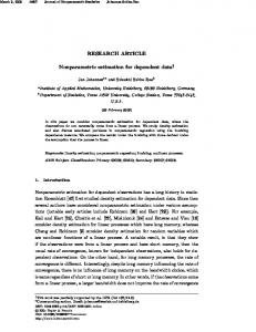
The data, kindly provided by Dr. Germaine Cornelissen-Guilaume of the University of Minnesota Chronobiology Laboratory, come from ambulatory monitoring equipment worn by a patient suffering from episodes of clinical depression. The time at which systolic blood pressure reaches its maximum value on a given day is called the ”acrophase”. Monitoring the acrophase for changes in the daily time of maximum can provide an automated early warning of a possible medical condition before it becomes clinically obvious. We show the results of a two-sided CUSUM analysis with reference constant ζ = 0.25 and control limits h = ± 8.59, which leads to an in-control ARL of approximately 500. The first m = 30 observations are used to find initial estimates of the required parameters. The left-hand panel in Figure 1 shows the CUSUM. The upper CUSUM + D signals at n = 66 and the changepoint estimate is τˆ = 57, that is, 27 observations after the warmup period. The right-hand panel in Figure 1 shows the CUSUM after restarting at n = 88, observations 58 through 87 serving as a warmup to estimate the new direction. A sustained decrease in the lower CUSUM D − is evident. The CUSUM signals at n = 120, a changepoint being indicated at n = 110. Continuing in this manner produces the results in Table 5, which shows the progress of the CUSUMs as the data accrue. The estimate of the mean direction in each segment is shown in the third column of the table.

17

15

10

10

5

5

0

0

-5

-5

-10

-10 30

35

40

45

50

55

60

65

-15 90

70

95

100

105

110

115

120

Figure 1 Direction CUSUMs of acrophase data. Left-hand panel: CUSUM after start at n = 31. right-hand panel: CUSUM after restart at n = 88. The vertical dotted lines indicate the location of the estimated changepoints. The dashed horizontal lines indicate the control limits. Table 5 Acrophase data: Progression of CUSUMs segment signal at νˆ 1 − 57 66 −1.7 58 − 110 120 −0.76 111 − 140 178 −1.9 141 − 241 255 −1.19 242 − 282 299 −0.90 Figure 2 shows a time series plot, constructed after the fact, of the mean directions in each of 30 contiguous groups of 10 observations each. The vertical dotted lines indicate segments delineated by the CUSUM. A noticeable feature in this plot is the three sets of more or less sustained increases followed by a sudden large decrease to a fixed level of about −2.75 radians. This is indicative of external interventions in the treatment of the patient to reset the acrophase. In retrospect, it seems that the CUSUMs have done a good job of identifying changes.

18

3

sample mean direction

2

1

0

-1

-2

-3 0

5

10

15

20

25

30

30 groups of 10 observations each

Figure 2 Plot of mean directions in 30 contiguous groups of . 10 observations each. The dotted lines delineate the segments identified by the CUSUM. In conclusion, the following remark is of some interest. Suppose the first 30 observations are treated as Phase I data. Then, the second factor on the right hand side of (11) is found to be 0.5 and ζ = 0.25 would be the suggested reference constant had the target out-of-control rotation been δ0 = 1 radian. The average estimated absolute direction change between the five identified segments is 0.77 radians, showing that the reference value ζ = 0.25 used in the CUSUM is not far off the supposed ”optimal” value.

4.2

Pulsar data

Lombard and Maxwell (2012) developed a cusum to detect deviation from a uniform distribution on the circle and applied it to some data consisting of arrival times of cosmic rays from the vicinity of a pulsar. The objective is to detect periods of sustained high energy radiation. Following a standard procedure in Astrophysics, the data were wrapped around a circle of circumference equal to the period of the pulsar. If no high energy radiation is present the wrapped data should be more or less uniformly distributed on the circumference of the circle, while a non-uniform distribution should manifest itself during periods of high energy radiation. They found that the first 190 observations could reasonably be assumed to have arisen from a 19

uniform distribution. We now apply to observations 191 through 1250 the concentration CUSUMs from Section 3 of the present paper to detect further changes in concentration. The in-control ARL of the chart is set at 500 observations with reference value ζ = 0 and control limits ±30.46. The first m = 50 observations are used to obtain initial estimates of the required means, variances and covariance of sin X and cos X. The full extent of the concentration CUSUM, without restarts, is shown in Figure 3. The first signal is at n = 191 + 495 = 686 and the changepoint is estimated at n = 191 + 331 = 522. The estimated concentration in the segment [192, 522] is 0.35. Thereafter, the lower CUSUM D − shows a sustained decrease to the end of the data series. In fact, if the CUSUM is restarted at n = 523, a changepoint is indicated at n = 523. Such a pattern is indicative of a more or less continuous decrease in concentration as the series progresses. The estimated concentration of the observations in the segment [523, 1250] is 0.06, suggesting a uniform distribution in this segment. Hawkins and Lombard (2015) applied a retrospective segmentation method to these data. Except for a short segment [191 − 207], which falls within the warmup set used to initiate the CUSUM, the results of the CUSUM analysis agree quite well with their results. 40 20 0 -20 -40 -60 -80 -100 -120 200

300

400

500

600

700

800

900

1000 1100 1200

Figure 3 Concentration CUSUM of the pulsar data.

20

Table 6 Pulsar data. Segments delineated by sequential CUSUM and retrospective segmentation Retrospective CUSUM segment νˆ κ ˆ segment νˆ κ ˆ 191-207 -0.41 1.89 208-573 -1.58 0.35 191-522 -1.44 0.35 574-1250 0.0 523-1250 0.06

5

Summary

We develop nonparametric CUSUMs for detecting changes in the mean direction and concentration of an angular distribution. The CUSUMs are designed for situations in which the initial mean direction and concentration are unspecified, the objective being to detect a change from the initial values. In this sense the CUSUMs are analogues of the self-starting CUSUMs of Hawkins (1987) for data from a normal distribution on the real line with unknown mean and variance. Monte Carlo simulation results indicate that the CUSUMs have in-control average run lengths that are acceptably close to the nominal values over a wide class of symmetric and asymmetric angular distributions. Two applications to data from Health Science and Astrophysics are discussed.

References [1] Abe, T. and Pewsey, A., (2011). Sine-skewed circular distributions. Statistics Papers, 52, 683–707. [2] Azzalini, A. and Capitanio,A., (2003). Distributions generated by perturbation of symmetry with emphasis on a multivariate skew t distribution Journal of the Royal Statistical Society,.B, 65, 367-389. [3] Hawkins, D. M., and Olwell, D. H., (1998). Cumulative Sum Charts and Charting for Quality Improvement, Springer Verlag, New York. [4] Hawkins, D.M., (1987). Self-Starting CUSUM Charts for Location and Scale. Journal of the Royal Statistical Society. Series D, 36, 299-316.

21

[5] Hawkins, D.M., Olwell, D. H. and Wang, B., (2016). http://cran.r-project.org/web/packages/CUSUMdesign/CUSUMdesign.pdf [6] Keefe, M.J., Woodall, W.H. and Jones-Farmer, L.A., (2015). The Conditional In-Control Performance of Self-Starting Control Charts. Quality Engineering, 27, 488-499. [7] Knoth,S., (2016). http://cran.r-project.org/web/packages/spc/spc.pdf [8] Hawkins, D M. and Lombard, F., (2015). Segmentation of circular data, Journal of Applied Statistics, 42 (1), 88-97. [9] Hawkins, D M. and Lombard, F., (2017). CUSUM control for data following the von Mises distribution. Journal of Applied Statistics. doi=10.1080/02664763.2016.1202217. To appear. [10] Helland, I., (1982). Central Limit Theorems for Martingales with Discrete or Continuous Time. Scandinavian Journal of Statistics, 9, 79-94. [11] Jammalamadaka, S. R., and SenGupta, A., (2001). Topics in Circular Statistics. Singapore: World Scientific Publishing Company. [12] Jones, M.C. and Faddy, M.J., (2003). A Skew Extension of the tDistribution, with Applications. Journal of the Royal Statistical Society, B, 65,159-174. [13] Lombard, F. and Maxwell, R.K., (2012). A CUSUM Procedure to Detect Deviations from Uniformity in Angular Data. Journal of Applied Statistics, 39, 1871-1880. [14] Lombard, F., Hawkins, D.M. and Potgieter, C.J. (2017). Sequential rank CUSUM charts for angular data. Computational Statistics and Data Analysis, 105, 268-279. [15] Mathworks: Matlab Version 2016b. [16] Nolan, J.P, (2015). Stable Distributions-Models for Heavy Tailed Data. Boston: Birkhauser. Note: In progress, Chapter 1 online at academic.2.american.edu/˜jpnolan. [17] Pewsey, A., (2000). The wrapped skew-normal distribution on the circle. Communications in Statistics - Theory and Methods, 29 (11), 2459-2472. 22

[18] Umbach, D. and Jammalamadaka, S.R., (2011). Building asymmetry into circular distributions. Statistics and Probability Letters, 79, 659663.

23