Sep 10, 2017 - â¤I am very grateful to my advisors, Donald Andrews and Edward Vytlacil, and ..... follows that g0(x) =
Nonparametric Estimation of Triangular Simultaneous Equations Models under Weak Identification Sukjin Han⇤ Department of Economics University of Texas at Austin
[email protected] September 10, 2017
Abstract This paper analyzes the problem of weak instruments on identification, estimation, and inference in a simple nonparametric model of a triangular system. The paper derives a necessary and sufficient rank condition for identification, based on which weak identification is established. Then, nonparametric weak instruments are defined as a sequence of reduced-form functions where the associated rank shrinks to zero. The problem of weak instruments is characterized as concurvity and to be similar to the ill-posed inverse problem, which motivates the introduction of a regularization scheme. The paper proposes a penalized series estimation method to alleviate the e↵ects of weak instruments and shows that it achieves desirable asymptotic properties. The findings of this paper provide useful implications for empirical work. To illustrate them, Monte Carlo results are presented and an empirical example is given in which the e↵ect of class size on test scores is estimated nonparametrically. Keywords: Triangular models, nonparametric identification, weak identification, weak instruments, series estimation, regularization, concurvity. JEL Classification Numbers: C13, C14, C36. ⇤ I am very grateful to my advisors, Donald Andrews and Edward Vytlacil, and committee members, Xiaohong Chen and Yuichi Kitamura for their inspiration, guidance and support. I am deeply indebted to Donald Andrews for his thoughtful advice throughout the project. The earlier version of this paper has benefited from discussions with Joseph Altonji, Ivan Canay, Philip Haile, Keisuke Hirano, Han Hong, Joel Horowitz, Seokbae Simon Lee, Oliver Linton, Whitney Newey, Byoung Park, Peter Phillips, Andres Santos, and Alex Torgovitsky. I gratefully acknowledge financial support from a Carl Arvid Anderson Prize from the Cowles Foundation. I also thank the seminar participants at Yale, UT Austin, Chicago Booth, Notre Dame, SUNY Albany, Duke, Sogang, SKKU, and Yonsei, as well as the participants at NASM and Cowles Summer Conference.
1
1
Introduction
Instrumental variables (IVs) are widely used in empirical research to identify and estimate models with endogenous explanatory variables. In linear simultaneous equations models, it is well known that standard asymptotic approximations break down when instruments are weak in the sense that (partial) correlation between the instruments and endogenous variables is weak. The consequences of and solutions for weak instruments in linear settings have been extensively studied in the literature over the past two decades; see, e.g., Bound et al. (1995), Staiger and Stock (1997), Dufour (1997), Kleibergen (2002, 2005), Moreira (2003), Stock and Yogo (2005), and Andrews and Stock (2007), among others. Weak instruments in nonlinear parametric models have recently been studied in the literature in the context of weak identification by, e.g., Stock and Wright (2000), Kleibergen (2005), Andrews and Cheng (2012), Andrews and Mikusheva (2016b,a), Andrews and Guggenberger (2015), and Han and McCloskey (2017). One might expect that nonparametric models with endogenous explanatory variables will generally require strong identification power as there is an infinite number of unknown parameters to identify, and hence, strong instruments may be crucial for a reasonable performance of estimation.1 Despite the problem’s importance and the growing popularity of nonparametric models, weak instruments in nonparametric settings have not received much attention.2 Furthermore, surprisingly little attention has been paid to the consequences of weak instruments in empirical research using nonparametric models; see below for references. Part of the neglect is due to the existing complications embedded in nonparametric models. In a simple nonparametric framework, this paper analyzes the problem of weak instruments on identification, estimation, and inference, and proposes an estimation strategy to mitigate the e↵ect. Identification results are obtained so that the concept of weak identification can subsequently be introduced via localization. The problem of weak instruments is characterized as concurvity and is shown to be similar to the ill-posed inverse problem. An estimation method is proposed through regularization and the resulting estimators are shown to have desirable asymptotic properties even when instruments are possibly weak. As a nonparametric framework, we consider a triangular simultaneous equations model. The specification of weak instruments is intuitive in the triangular model because it has an explicit reduced-form relationship. Additionally, clear interpretation of the e↵ect of weak instruments can be made through a specific structure produced by the control function approach. To make our analysis succinct, we specify additive errors in the model. This particular model is considered in Newey et al. (1999) (NPV) and Pinkse (2000) in a situation without weak instruments. Although relatively recent 1
This conjecture is shown to be true in the setting considered in this paper; see Theorem 5.1 and Corollary 5.2. Chesher (2003, 2007) mentions the issue of weak instruments in applying his key identification condition in the empirical example of Angrist and Keueger (1991). Blundell et al. (2007) determine whether weak instruments are present in the Engel curve dataset of their empirical section. They do this by applying the Stock and Yogo (2005) test developed in linear models to their reduced form, which is linearized by sieve approximation. Darolles et al. (2011) briefly discuss weak instruments that are indirectly characterized within their source condition. 2
2
developments in nonparametric triangular models contribute to models with nonseparable errors (e.g., Imbens and Newey (2009), Kasy (2014)), such flexibility complicates the exposition of the main results of this paper.3 Also, having a form analogous to its popular parametric counterpart, the model with additive errors is broadly used in applied research such as Blundell and Duncan (1998), Yatchew and No (2001), Lyssiotou et al. (2004), Dustmann and Meghir (2005), Skinner et al. (2005), Blundell et al. (2008), Del Bono and Weber (2008), Frazer (2008), Mazzocco (2012), Coe et al. (2012), Breza (2012), Henderson et al. (2013), Chay and Munshi (2014), and Koster et al. (2014). One of the contributions of this paper is that it derives novel identification results in nonparametric triangular models that complement the existing results in the literature. With a mild support condition, we show that a particular rank condition is necessary and sufficient for the identification of the structural relationship. This rank condition is substantially weaker than what is established in NPV. The rank condition covers economically relevant situations such as outcomes resulting from corner solutions or kink points in certain economic models. More importantly, deriving such a rank condition is the key to establishing the notion of weak identification. Since the condition is minimal, a “slight violation” of it has a binding e↵ect on identification, hence resulting in weak identification. To characterize weak identification, we consider a drifting sequence of reduced-form functions that converges to a non-identification region, namely, a space of reduced-form functions that violate the rank condition for identification. A particular rate is designated relative to the sample size, which e↵ectively measures the strength of the instruments, so that it appears in asymptotic results for the estimator of the structural function. The concept of nonparametric weak instruments generalizes the concept of weak instruments in linear models such as in Staiger and Stock (1997). In the nonparametric control function framework, the problem of weak instruments becomes a nonparametric analogue of a multicollinearity problem known as concurvity (Hastie and Tibshirani (1986)). Once the endogeneity is controlled by a control function, the model can be rewritten as an additive nonparametric regression, where the endogenous variables and reduced-form errors comprise two regressors, and weak instruments result in the variation of the former regressor being mainly driven by the variation of the latter. This problem of concurvity is related to the illposed inverse problem inherent in other nonparametric models with endogeneity or, in general, to settings where smoothing operators are involved; see Carrasco et al. (2007) or Chen and Reiss (2011). Although the sources of ill-posedness in the two problems are di↵erent, there is sufficient similarity that the regularization methods used in the literature to solve the ill-posed inverse problem can be introduced to our problem. Due to the problems’ distinct features, however, among the regularization methods, only penalization (i.e., Tikhonov-type regularization) alleviates the e↵ect of weak instruments. 3 For instance, the control function employed in Imbens and Newey (2009) requires large variation in instruments, and hence discussing weak instruments (i.e., weak association between endogenous variables and instruments or little variation in instruments) in such a context requires more care.
3
This paper proposes a penalized series estimator for the structural function and establishes its asymptotic properties. We develop a modified version of the standard L2 penalization to control the penalty bias. Our results on the rate of convergence of the estimator suggest that, without penalization, weak instruments characterized as concurvity slow down the overall convergence rate, exacerbating bias and variance “symmetrically.” We then show that a faster convergence rate is achieved with penalization than without, while the penalty bias can be dominated by the standard approximation bias. We also derive consistency and asymptotic normality with mildly weak instruments. The problem of concurvity in additive nonparametric models is also recognized in the literature where di↵erent estimation methods are proposed to address the problem—e.g., the backfitting methods (Linton (1997), Nielsen and Sperlich (2005)) and the integration method (Jiang et al. (2010)); also see Sperlich et al. (1999). In particular, as closely related work to the asymptotic results of this paper, Jiang et al. (2010) establish pointwise asymptotic normality for local linear and integral estimators in an additive nonparametric model with highly correlated covariates. In the present paper, where an additive model results from a triangular model accompanied with the control function approach, the problem of concurvity is addressed in a more direct manner via penalization. In addition, although the main conclusions of this paper do not depend on the choice of nonparametric estimation method, using series estimation in our penalization procedure is also justified in the context of design density. In situations where the joint density of x and v becomes singular, such as in our case with weak instruments, it is known that series and local linear estimators are less sensitive than conventional kernel estimators; see, e.g., Hengartner and Linton (1996) and Imbens and Newey (2009) for related discussions. Another possible nonparametric framework in which to examine the problem of weak instruments is a nonparametric IV (NPIV) model (Newey and Powell (2003), Hall and Horowitz (2005) and Blundell et al. (2007), among others). Unlike in a triangular model, the absence of an explicit reduced-form relationship forces weak instruments in this setting to be characterized as a part of the ill-posed inverse problem. Therefore, in this model, the performance of the estimator can be severely deteriorated as the problem is “doubly ill-posed.”4 Further, it may also be hard to separate the e↵ects of the two in asymptotic theory. As a related recent work, Freyberger (2015) provides a framework by which the completeness condition can be tested in a NPIV model. Instead of using a drifting sequence of distributions, he indirectly defines weak instruments as a failure of a restricted version of the completeness condition. While he applies his framework to test weak instruments, our focus is on estimation and inference of the function of interest in a di↵erent nonparametric model with a more explicit definition of weak instruments. The findings of this paper provide useful implications for empirical work. First, when estimating a nonparametric structural function, the results of IV estimation and subsequent inference can be 4
In Section 8, we illustrate this point in an empirical application by comparing estimates calculated from the triangular and NPIV models.
4
misleading even when the instruments are strong in terms of conventional criteria for linear models.5 Second, the symmetric e↵ect of weak instruments on bias and variance implies that the bias–variance trade-o↵ is the same across di↵erent strengths of instruments, and hence, weak instruments cannot be alleviated by exploiting the trade-o↵. Third, penalization on the other hand can alleviate weak instruments by significantly reducing variance and sometimes bias as well. Fourth, there is a tradeo↵ between the smoothness of the structural function (or the dimensionality of its argument) and the requirement of strong instruments. Fifth, if a triangular model along with its assumptions is considered to be reasonable, it makes the data to be informative about the relationship of interest more than a NPIV model does, which is an attractive feature especially in the presence of weak instruments. Sixth, although a linear first-stage reduced form is commonly used in applied research (e.g., in NPV, Blundell and Duncan (1998), Blundell et al. (1998), Dustmann and Meghir (2005), Coe et al. (2012), and Henderson et al. (2013)), the strength of instruments can be improved by having a nonparametric reduced form so that the nonlinear relationship between the endogenous variable and instruments can be fully exploited. The last point is related to the identification results of this paper. In Section 8, we apply the findings of this paper to an empirical example, where we nonparametrically estimate the e↵ect of class size on students’ test scores. The rest of the paper is organized as follows. Section 2 introduces the model and obtains new identification results. Section 3 discusses weak identification and Section 4 relates the weak instrument problem to the ill-posed inverse problem and defines our penalized series estimator. Sections 5 and 6 establish the rate of convergence and consistency of the penalized series estimator and the asymptotic normality of some functionals of it. Section 7 presents the Monte Carlo simulation results. Section 8 discusses the empirical application. Finally, Section 9 concludes.
2
Identification
We consider a nonparametric triangular simultaneous equations model y = g0 (x, z1 ) + ",
x = ⇧0 (z) + v,
E["|v, z] = E["|v] a.s.,
E[v|z] = 0 a.s.,
(2.1a) (2.1b)
where g0 (·, ·) is an unknown structural function of interest, ⇧0 (·) is an unknown reduced-form
function, x is a dx -vector of endogenous variables, z = (z1 , z2 ) is a (dz1 + dz2 )-vector of exogenous variables, and z2 is a vector of excluded instruments. The stochastic assumptions (2.1b) are more general than the assumption of full independence between (", v) and z and E[v] = 0. Following the 5
For instance, in Coe et al. (2012), the first-stage F -statistic value that is reported is (sometimes barely) in favor of strong instruments, but the judgement is based on the criterion for linear models. The majority of empirical works referenced above do not report first-stage results.
5
control function approach, E[y|x, z] = g0 (x, z1 ) + E["|⇧0 (z) + v, z] = g0 (x, z1 ) + E["|v] = g0 (x, z1 ) + where
0 (v)
0 (v),
(2.2)
= E["|v] and the second equality is from the first part of (2.1b). In e↵ect, we capture
endogeneity (E["|x, z] 6= 0) by an unknown function
0 (v),
which serves as a control function. Once
v is controlled for, the only variation of x comes from the exogenous variation of z. Based on equation (2.2) we establish identification, weak identification, and estimation results. First, we obtain identification results that complement the results of NPV. For useful comparisons, we first restate the identification condition of NPV which is written in terms of ⇧0 (·). Given (2.2), the identification of g0 (x, z1 ) is achieved if one can separately vary (x, z1 ) and v in g(x, z1 ) + (v). Since x = ⇧0 (z) + v, a suitable condition on ⇧0 (·) will guarantee this via the separate variation of z and v. In light of this intuition, NPV propose the following identification condition. Proposition 2.1 (Theorem 2.3 in NPV) If g(x, z1 ), (v), and ⇧(z) are di↵erentiable, the boundary of the support of (z, v) has probability zero, and
Pr rank
✓
@⇧0 (z) @z20
◆
= dx = 1,
(2.3)
then g0 (x, z1 ) is identified up to an additive constant. The identification condition can be seen as a nonparametric generalization of the rank condition. One can readily show that the order condition (dz2
dx ) is incorporated in this rank condition.
Note that this condition is only a sufficient condition, which suggests that the model can possibly be identified with a relaxed rank condition. This observation motivates our identification analysis. We find a necessary and sufficient rank condition for identification by introducing a mild support condition. The identification analysis of this section is also important for our later purpose of defining the notion of weak identification. Henceforth, in order to keep our presentation succinct, we focus on the case where the included exogenous variable z1 is dropped from model (2.1) and z = z2 . With z1 included, all the results of this paper readily follow similar lines; e.g., the identification analysis follows conditional on z1 . We first state and discuss the assumptions that we impose. Assumption ID1 The functions g0 (x),
0 (v),
and ⇧0 (z) are continuously di↵erentiable in their
arguments. This condition is also assumed in Proposition 2.1 above. Before stating a key additional assumption for identification, we first define the supports that are associated with x and z. Let X ⇢ Rdx
and Z ⇢ Rdz be the marginal supports of x and z, respectively. Also, let Xz be the conditional 6
support of x given z 2 Z. We partition Z into two regions where the rank condition is satisfied, i.e., where z is relevant, and otherwise.
Definition 2.1 (Relevant set) Let Z r be the subset of Z defined by r
r
Z = Z (⇧0 (·)) =
⇢
z 2 Z : rank
✓
@⇧0 (z) @z 0
◆
= dx .
Let Z 0 = Z\Z r be the complement of the relevant set. Let X r be the subset of X defined by
X r = {x 2 Xz : z 2 Z r }. Given the definitions, we introduce an additional support condition.
Assumption ID2 The supports X and X r di↵er only on a set of probability zero, i.e., Pr [x 2 X \X r ] = 0.
Intuitively, when z is in the relevant set, x = ⇧0 (z) + v varies as z varies, and therefore, the support of x corresponding to the relevant set is large. Assumption ID2 assures that the corresponding support is large enough to almost surely cover the entire support of x. ID2 is not as strong as it may appear to be. Below, we show this by providing mild sufficient conditions for ID2. If we identify g0 (x) for any x 2 X r , then we achieve identification of g0 (x) by Assumption ID2.6
Now, in order to identify g0 (x) for x 2 X r , we need a rank condition, which will be minimal. The following is the identification result:
Theorem 2.2 In model (2.1), suppose Assumptions ID1 and ID2 hold. Then, g0 (x) is identified on X up to an additive constant if and only if
Pr rank
✓
@⇧0 (z) @z 0
◆
= dx > 0.
(2.4)
This and all subsequent proofs can be found in Appendix A below and more can be found in Appendix B (Supplemental Appendix). The rank condition (2.4) is necessary and sufficient. By Definition 2.1, it can alternatively be written as Pr [z 2 Z r ] > 0. The condition is substantially weaker than (2.3) in Proposition 2.1, which is Pr [z 2 Z r ] = 1 (with z = z2 ). That is, Theorem 2.2 extends the result of NPV in the sense that when Z r = Z, ID2 is trivially satisfied with X = X r . Theorem 2.2 shows that it is enough
for identification of g0 (x) to have any fixed positive probability with which the rank condition is satisfied.7 This condition can be seen as the local rank condition as in Chesher (2003), and we achieve global identification with a local rank condition. Although this gain comes from having the additional support condition, the trade-o↵ is appealing given the later purpose of building a weak 6 The support on which an unknown function is identified is usually left implicit in the literature. To make it more explicit, g0 (x) is identified if g0 (x) is identified on the support of x almost surely. 7 A similar condition appears in the identification analysis of Hoderlein (2009), where endogenous semiparametric binary choice models are considered in the presence of heteroskedasticity.
7
identification notion. Even without Assumption ID2, maintaining the assumptions of Theorem 2.2, we still achieve identification of g0 (x), but on the set {x 2 X r }.
Lastly, in order to identify the level of g0 (x), we need to introduce some normalization as in NPV. Either E["] = 0 or 0 (¯ v ) = ¯ suffices to pin down g0 (x). With the latter normalization, it follows that g0 (x) = E[y|x, v = v¯] ¯ , which we apply in estimation as it is convenient to implement. The following is a set of sufficient conditions for Assumption ID2. Let Vz be the conditional
support of v given z 2 Z.
Assumption ID20 Either (a) or (b) holds. (a) (i) x is univariate and x and v are continuously distributed, (ii) Z is a cartesian product of connected intervals, and (iii) Vz = Vz˜ for all z, z˜ 2 Z 0 ; (b) Vz = Rdx for all z 2 Z.
Lemma 2.1 Under Assumption ID1, Assumption ID20 implies Assumption ID2. In Assumption ID20 , the continuity of the r.v. is closely related to the support condition in Proposition 2.1 that the boundary of support of (z, v) has probability zero. For example, when z or v is discrete their condition does not hold. Assumption ID20 (a)(i) assumes that the endogenous variable is univariate, which is most empirically relevant in nonparametric models. An additional condition is required with multivariate x, which is omitted in this paper. Even under ID20 (a)(i), however, the exogenous covariate z1 in g(x, z1 ), which is omitted in the discussion, can still be a vector. ID20 (a)(ii) and (iii) are rather mild. ID20 (a)(ii) assumes that z has a connected support, which in turn requires that the excluded instruments vary smoothly. The assumptions on the continuity of the r.v. and the connectedness of Z are also useful in deriving the asymptotic theory
of the series estimator considered in this paper; see Assumption B below. ID20 (a)(iii) means that the conditional support of v given z is invariant when z is in Z 0 . This support invariance condition is the key to obtaining a rank condition that is considerably weaker than that of NPV. Our support
invariance condition is di↵erent from the support invariance condition introduced in Imbens and Newey (2009). Using the notations of the present paper, Imbens and Newey (2009) require that the support of v conditional on x equals the marginal support of v, which inevitably requires a large support of z. On the other hand, ID20 (a)(iii) requires that the support of v conditional on z is invariant (for z 2 Z 0 ), and therefore imposes no restriction on the support of z. Also, the conditional support does not have to equal the marginal support of v here. ID20 (a)(iii), along with the control
function assumptions (2.1b), is a weaker orthogonality condition for z than the full independence condition z ? v. Note that Vz = {x
⇧0 (z) : x 2 Xz }. Therefore, ID20 (a)(iii) equivalently means
that Xz is invariant for those z satisfying E[x|z] = const. Moreover, one can introduce a condition that is weaker than ID20 (a)(iii): Xz ⇢ X r for those z satisfying E[x|z] = const.8 These conditions in terms of Xz can be checked from the data.
Therefore, heteroskedasticity of v may in general violate ID2 and thus ID20 (a)(iii), although some types heteroskedasticity can still be allowed (e.g., heteroskedasticity only when z is relevant). 8
8
Figure 1: Identification under Assumption ID20 (a), univariate z and no z1 . Given ID20 (b) that v (and thus x) has a full conditional support, ID2 is trivially satisfied and no additional restriction is imposed on the joint support of z and v. ID20 (b) also does not require univariate x or the connectedness of Z. This assumption on Vz is satisfied with, for example, a normally distributed error term (conditional on regressors).
Figure 1 illustrates the intuition of the identification proof under ID20 (a) in a simple case where z is univariate. With ID20 (b), the analysis is even more straightforward; see the proof of Lemma 2.1 in Appendix A. In the figure, the local rank condition (2.4) ensures global identification of g0 (x). The intuition is as follows. First, by @E[y|v, z]/@z = (@g0 (x)/@x) · (@⇧0 (z)/@z) and the rank
condition, g0 (x) is locally identified on x corresponding to a point of z in the relevant set Z r . As such a point of z varies within Z r , the x corresponding to it also varies enough to cover almost the
entire support of x. At the same time, for any x corresponding to an irrelevant z (i.e., z outside of Z r ), one can always find z inside of Z r that gives the same value of such an x. The probability
Pr [z 2 Z r ] being small but bounded away from zero only a↵ects the efficiency of estimators in the estimation stage. This issue is related to the weak identification concept discussed later.
Note that the strength of identification of g0 (x) is di↵erent for di↵erent subsets of X . For
instance, identification must be strong in a subset of X corresponding to a subset of Z where
⇧0 (·) is steep. In addition, g0 (x) is over-identified on a subset of X that corresponds to multiple
subsets of Z where ⇧0 (·) has a nonzero slope, since each association of x and z contributes to identification. This discussion implies that the shape of ⇧0 (·) provides useful information on the
strength of identification in di↵erent parts of the domain of g0 (x). Lastly, it is worth mentioning that the separable structure of the reduced form along with ID20 (a)(iii) allows “global extrapolation” in a manner that is analogous to that in a linear model. The identification results of this section apply to economically relevant situations. Let x be an economic agent’s optimal decision induced by an economic model and z be a set of exogenous components in the model that a↵ects the decision x. One is interested in a nonlinear e↵ect of the 9
optimal choice on a certain outcome y in the model. We present two situations where the resulting Pr [z 2 Z r ] is strictly less than unity in this economic problem: (a) x is realized as a corner solution beyond a certain range of z. In a returns-to-schooling example, x can be the schooling decision of a potential worker, z the tuition cost or distance to school, and y the future earnings. When the tuition cost is too high or the distance to school is too far beyond a certain threshold, such an instrument may no longer a↵ect the decision to go to school. (b) The budget set has kink points. In a labor supply curve example, x is the before-tax income, which is determined by the labor supply decision, z the worker’s characteristics that shift her utility function, and y the wage. If an income tax schedule has kink points, then the x realized at such points will possibly be invariant at the shift of the utility. The identification results of this paper imply that even in these situations, the returns to schooling or the labor supply curve can be fully identified nonparametrically as long as Pr [z 2 Z r ] > 0.
3
Weak Identification
The previous section discusses the structure of the joint distribution of x and z that contributes to the identification of g0 (·). Specifically, (2.4) imposes a minimal restriction on the shape of the conditional mean function E[x|z] = ⇧0 (z). This necessity result suggests that “slight violation” of (2.4) will result in weak identification of g0 (·). Note that this approach will not be successful with (2.3) of NPV, since violating the condition, i.e., Pr [rank (@⇧0 (z)/@z 0 ) = dx ] < 1, can still result in strong identification. In this section, we formally construct the notion of weak identification via localization. We define nonparametric weak instruments as a drifting sequence of reduced-form functions that are localized around a function with no identification power. Such a sequence of models or drifting data-generating process (Davidson and MacKinnon (1993)) is introduced to define weak instruments relative to the sample size n. As a result, the strength of instruments is represented in terms of the rate of localization, and hence, it can eventually be reflected in the local asymptotics of the estimator of g0 (·). Let C(Z) be the class of conditional mean functions ⇧(·) on Z that are bounded, Lipschitz
and continuously di↵erentiable. Define a non-identification region C0 (Z) as a class of functions that satisfy the lack-of-identification condition motivated by (2.4)9 : C0 (Z) = {⇧(·) 2 C(Z) :
Pr [rank (@⇧(z)/@z 0 ) < dx ] = 1}. Define an identification region as C1 (Z) = C(Z)\C0 (Z). We consider a sequence of triangular models y = g0 (x) + " and x = ⇧n (z) + v with corresponding stochastic assumptions. Although g(x) is identified with ⇧n (·) 2 C1 (Z) for any fixed n by Theorem 2.2, g(x) is ¯ in C0 (Z). Namely, the noise (i.e., v) cononly weakly identified as ⇧n (·) drifts toward a function ⇧(·)
tributes more than the signal (i.e., ⇧n (z)) to the total variation of x 2 {⇧n (z) + v : z 2 Z, v 2 V} 9
The lack of identification condition is satisfied either when the order condition fails (dz < dx ), or when z are jointly irrelevant for one or more of x, almost everywhere in their support.
10
as n ! 1. In order to facilitate a meaningful asymptotic theory in which the e↵ect of weak instruments is reflected, we further proceed by considering a specific sequence of ⇧n (·).
Assumption L (Localization) For some > 0, the true reduced-form function ⇧n (·) satisfies ˜ 2 C1 (Z) that does not depend on n and for z 2 Z the following. For some ⇧(·) @⇧n (z) =n @z 0
˜ @ ⇧(z) + op (n @z 0
).
˜ · ⇧(z) + c + op (n
)
·
Assumption L is equivalent to ⇧n (z) = n
(3.1)
for some constant vector c. This specification of a uniform convergent sequence over Z can be justified by our identification analysis. The “local nesting” device in (3.1) is also used in Stock and
Wright (2000) and Jun and Pinkse (2012) among others. In contrast to these papers, the value measures the strength of identification here and is not specified to be 1/2.10 Unlike a linear
of
reduced form, to characterize weak instruments in a more general nonparametric reduced form, we need to control the complete behavior of the reduced-form function, and the derivation of local asymptotic theory seems to be more demanding. Nevertheless, the particular sequence considered in Assumption L makes the weak instrument asymptotic theory straightforward while embracing the most interesting local alternatives against non-identification.11
4
Estimation
Once the endogeneity is controlled by the control function in (2.2), the problem becomes one of estimating the additive nonparametric regression function E[y|x, z] = g0 (x) +
0 (v).
In a weak
instrument environment, however, we face a nonstandard problem called concurvity: x = ⇧n (z) + v ! v a.s. as n ! 1 under the weak instrument specification (3.1) of Assumption L with c = 0 P as normalization. With a series representation g0 (x) + 0 (v) = 1 j=1 { 1j pj (x) + 2j pj (v)}, where the pj (·)’s are the approximating functions, it becomes a familiar problem of multicollinearity as
pj (x) ! pj (v) a.s. for all j. More precisely, pj (x) pj (v) = Oa.s. (n ) by mean value expansion ˜ ˜ pj (v) = pj (x n ⇧(z)) = pj (x) n ⇧(z)@p x)/@x with an intermediate value x ˜. Alternatively, j (˜ by plugging this expression of pj (v) back into the series, we can see that the variation of the regressor It would be interesting to have di↵erent rates across columns or rows of @⇧@zn0(·) . One can also consider di↵erent rates for di↵erent elements of the matrix. The analyses in these cases can analogously be done by slight modifications of the arguments. 11 In defining weak instruments in Assumption L, one can consider an intermediate case where @⇧@zn0(·) converges to a matrix with reduced-rank rather than that with zero rank. Extending the analysis in this case can follow analogously but omitted in the paper for succinctness. 10
11
shrinks as n ! 1. This feature is reminiscent of the ill-posed inverse problem that commonly occurs,
e.g., in estimating a standard NPIV model of y = g0 (x) + " with endogenous x and E["|z] = 0. By P P1 writing g0 (x) = 1 j=1 1j pj (x) it follows that E[y|z] = j=1 1j E [pj (x)|z]. Analogous to the weak ⇥ ⇤ instruments problem, the variation of the regressor E [pj (x)|z] shrinks since E E[pj (x)|z]2 ! 0 as j ! 1 (Kress (1999, p. 235)). Blundell and Powell (2003, p. 321) also acknowledge that the ill-posed inverse problem is a functional analogue to the multicollinearity problem.
Given the connections between the weak instruments, concurvity, and ill-posed inverse problems, the regularization methods used in the realm of research concerning inverse problems are suitable for use with weak instruments. There are two types of regularization methods used in the literature: the truncation method and the penalization method.12 In this paper, we introduce the penalization scheme. The nature of our problem is such that the truncation method does not work properly. Unlike in the ill-posed inverse problem, we still have the concurvity problem even after truncating the series, since pj (x) ! pj (v) a.s. even for j J < 1 as n ! 1. On the other hand, the penalization directly controls the behavior of the
1j ’s
and
2j ’s,
and hence, it successfully regularizes the weak
instrument problem. We propose a penalized series estimation procedure for h0 (w) = g0 (x) +
0 (v)
where w = (x, v).
We choose to use series estimation rather than other nonparametric methods as it is more suitable in our particular framework. Because x ! v a.s. the joint density of w becomes concentrated along a lower dimensional manifold as n tends to infinity. As mentioned in the introduction, series estimators are less sensitive to this problem of singular density. See Assumption B below for related discussions. Furthermore with series estimation, it is easy to impose the additivity of h0 (·) and to characterize the problem of weak instruments as a multicollinearity problem. The estimation procedure takes two steps. In the first stage, we estimate the reduced form ⇧n (·) using a standard series estimation method and obtain the residual vˆ. In the second stage, we estimate the structural function h0 (·) using a penalized series estimation method with w ˆ = (x, vˆ) as the regressors. The theory that follows uses orthonormal polynomials as approximating functions. Let {(yi , xi , zi )}ni=1 be the data with n observations, and let rL (zi ) = (r1 (zi ), ..., rL (zi ))0 be a vector
of approximating functions of order L for the first stage. Define a matrix R = (rL (z1 ), ..., rL (zn ))0 . rL (z
L 0 0 ˆ i ) gives ⇧(·) = r (·) ˆ where ˆ = (R R)
n⇥L 1 R0 (x , ..., x )0 , 1 n
Then, regressing xi on and we obtain ˆ vˆi = xi ⇧(zi ). Define a vector of approximating functions of order K for the second stage as pK (w) = (p1 (w), ..., pK (w))0 . To reflect the additive structure of h0 (·), there are no interaction terms between the approximating functions for g0 (·) and those for
0 (·)
in this vector; see Appendix A for the explicit expression. Denote a matrix of approximating functions as Pˆ = (pK (w ˆ1 ), ..., pK (w ˆn ))0 n⇥K
where w ˆi = (xi , vˆi ). Note that L = L(n) and K = K(n) grow with n. 12 In Chen and Pouzo (2012) closely related concepts are used in di↵erent terminologies: minimizing a criterion over finite sieve space and minimizing a criterion over infinite sieve space with a Tikhonov-type penalty.
12
We define a penalized series estimator : ˆ ⌧ (w) = pK (w)0 ˆ⌧ , h
(4.1)
where the “interim” estimator ˆ⌧ optimizes a penalizing criterion function ˆ⌧ = arg min
˜2RK
⇣
y
⌘0 ⇣ Pˆ ˜ y
⌘ Pˆ ˜ /n + ⌧n ˜0 DK ⇤ ˜,
(4.2)
where y = (y1 , ..., yn )0 , DK ⇤ = Diag{0, ..., 0, 1, ..., 1} is a diagonal matrix that satisfies ˜0 DK ⇤ ˜ = PK ˜2 0 the penalization parameter. In (4.2), the standard L2 penalty is tailored j=K ⇤ +1 j , and ⌧n to meet our purpose. We introduce such a modification and allow K ⇤ = K ⇤ (n) to grow with
n to gain sufficient control over the bias created by the penalization in this nonparametric weak instrument setting; see Assumption G below for related discussions. Note that the penalty term ⌧n ˜0 DK ⇤ ˜ penalizes the coefficients on the higher-order series, which e↵ectively imposes smoothness restrictions on h0 (·). For the same purpose of controlling the bias, ⌧n is assumed to converge to zero. The optimization problem (4.2) yields a closed form solution: ˆ⌧ = (Pˆ 0 Pˆ + n⌧n DK ⇤ )
1
Pˆ 0 y.
The multicollinearity feature discussed above is manifested here by the fact that the matrix Pˆ 0 Pˆ is nearly singular under Assumption L, since the two columns of Pˆ become nearly identical. In terms of ⇥ ⇤ the population second moment matrix Q = E pK (wi )pK (wi )0 , the challenge is that the minimum eigenvalue of Q is not bounded away from zero, which is manifested as in Lemma A.2 in Appendix A) where
max
max (Q
1)
= O(n2 ) (shown
denotes the maximum eigenvalue. The term n⌧n DK ⇤
mitigates such singularity, without which the performance of the estimator of h0 (·) would deteriorate severely.13 The relative e↵ects of weak instruments (n2 ) and penalization (⌧n ) will determine the ˆ ⌧ (·). Given h ˆ ⌧ (·), with the normalization that (¯ asymptotic performance of h v ) = ¯ , we have ˆ ⌧ (x, v¯) ¯ . gˆ⌧ (x) = h
5
Consistency and Rate of Convergence
First, we state the regularity conditions and key preliminary results under which we find the rate of convergence of the penalized series estimator introduced in the previous section. Let X = (x, z). Assumption A {(yi , xi , zi ) : i = 1, 2, ...} are i.i.d. and var(x|z) and var(y|X) are bounded func13
In linear settings, the introduction of a regularization method is less appealing as it creates the well-known biased estimator of ridge regression. In contrast, we do not directly interpret ˆ⌧ in the current nonparametric setting, since ˆ ⌧ (·). More importantly, the overall bias of h ˆ ⌧ (·) is unlikely to it is only an interim estimator calculated to obtain h be worsened in the sense that the additional bias introduced by penalization can be dominated by the existing series estimation bias.
13
tions of z and X, respectively. Assumption B (z, v) is continuously distributed with density that is bounded away from zero on Z ⇥ V, and Z ⇥ V is a cartesian product of compact, connected intervals. Assumption B is useful to bound below and above the eigenvalues of the “transformed” second moment matrix of approximating functions. This condition is worthy of discussion in the context of identification and weak identification. Let fu and fw denote the density functions of u = (z, v) and w = (x, v), respectively. An identification condition like Assumption ID20 in Section 2 is embodied in Assumption B. To see this, note that fu being bounded away from zero means that there is no functional relationship between z and v, which in turn implies Assumption ID20 (a)(iii).14 On the other hand, an assumption written in terms of fw like Assumption 2 in NPV (p. 574) cannot be imposed here. Observe that w = (⇧n (z) + v, v) depends on the behavior of ⇧n (·), and hence fw is not bounded away from zero uniformly over n under Assumption L and approaches a singular density. Technically, making use of a transformation matrix (see Appendix A), an assumption is made in terms of fu , which is not a↵ected by weak instruments, and the e↵ect of weak instruments can be handled separately in the asymptotics proof. Note that the assumption for the Cartesian products of supports, namely Z ⇥ V and its compactness can be replaced by introducing a trimming function as in NPV, that ensures bounded rectangular supports.15 Assumption B can be weakened
to hold only for some component of the distribution of z; some components of z can be allowed to be discrete as long as they have finite supports. Next, Assumption C is a smoothness assumption on the structural and reduced-form functions. P For a generic dimension d and a d-vector µ of nonnegative integers, let |µ| = dl=1 µl . Define the µ
derivative @ µ g(x) = @ |µ| g(x)/@xµ1 1 @xµ2 2 · · · @xdxdx of order |µ|. Let !(·) be a positive continuous ´ 0 weight function on X and let kgkX ,! = X |@ (1,...,1) g(x)|!(x)dx be a weighted seminorm of g(·); for an univariate example of this seminorm, see (4.5) of Trefethen (2008). Let W be the support of w = (x, v).
Assumption C g0 (x) and s on W, and
k@ µ gkX ,!
+
0 (v) are µ k@ kV,! is
Lipschitz and absolutely continuously di↵erentiable of order bounded by a fixed constant for |µ| = s. ⇧n (z) is bounded,
Lipschitz, and absolutely continuously di↵erentiable of order s⇡ on Z, and for the m-th element ⇧n,m (z), k@ µ ⇧n,m kZ,! is bounded by a fixed constant for |µ| = s⇡ , and for all n and m dx .
As shown in the following lemma, this assumption on di↵erentiability and bounded variation ensures that the coefficients on the series expansions have particular decay rates and that the approximation errors shrink at particular rates as the number of approximating functions increases. Recall that pj (w) and rj (z) are (the tensor products of) orthogonal polynomials on W and Z, 14
The definition of a functional relationship can be found, e.g., in NPV (p. 568). Assumption ID20 (b) is then viewed to hold for h(w) multiplied by a trimming function, thus identification is still achieved over the trimmed support. 15
14
respectively. We present results for the Chebyshev polynomials here, and results for the Legendre polynomials can be found in Appendix B. Lemma 5.1 Under Assumptions B and C,
P1
j=1
j pj (w)
of h0 (w) and
P1
j=1 nj rj (z)
all n are uniformly convergent, and for a generic positive constant c and for all n, (i) and
nl
cl
s⇡ /dz 1 ;
(ii) supw2W h0 (w)
PK˜
j=1
j pj (w)
˜ and L. ˜ for all positive integers K
˜ cK
s/dx
and supz2Z ⇧n (z)
j
of ⇧n (z) for s/dx 1
cj
PL˜
j=1 nj rj (z)
˜ cL
s⇡ /dz
Lemma 5.1(i) is closely related to the assumptions on the decay rate of coefficients in the literature. For example, Hall and Horowitz (2005) assume that the rate is O(j
) for some constant
> 1/2. Such an assumption is an abstract assumption on smoothness and is agnostic about dimensionality. This paper does not assume but explicitly derives the decay rate from a conventional smoothness condition of Assumption C. The rate is also informative about dimensionality. The decay rate is useful later in showing that the rate of the penalty bias is dominated by the rate of the approximation bias. The approximation error bound of (ii) is implied from (i).16 In Lemma 5.1(i) and hence in (ii), the dimension of w is reduced to the dimension of x as the additive structure of h0 (w) is exploited; see e.g., Andrews and Whang (1990). p Assumption D n K 7/2 ( L/n+L s⇡ /dz ) ! 0 and n K 11/2 ! 0. Also, ⌧n ! 0 and K > 2(K ⇤ +1) for any n.
Assumption D restricts the rate of growth of the numbers K and L of the approximating functions. The conditions on K and L are more restrictive than the corresponding assumption for the power series in NPV (Assumption 4, p. 575) where weak instruments are not considered. Now, ˆ ⌧ (w) we provide results for the rate of convergence in probability of the penalized series estimator h in terms of L2 and uniform distance. Let F (w) = Fw (w) for simplicity. Theorem 5.1 Suppose Assumptions A–D and L are satisfied. Let Rn = min{n , ⌧n ⇢ˆ h
ˆ ⌧ (w) h
h0 (w)
i2
dF (w)
1 2
⇣ p = Op Rn ( K/n + K
s dx
s dx
+ ⌧n R n K ⇤
1 2
+
1/2
}. Then
p L/n + L
s⇡ dz
⌘ ) .
Also, ˆ ⌧ (w) sup h
w2W
⇣ p h0 (w) = Op Rn K( K/n + K
s dx
+ ⌧n R n K ⇤
s dx
1 2
+
p L/n + L
s⇡ dz
⌘ ) .
Suppose there is no penalization (⌧n = 0). Then with Rn = Op (n ), Theorem 5.1 provides the ˆ rates of convergence of the unpenalized series estimator h(·). For example, with k·kL2 denoting the 16 No result analogous to (i) is derived in Lorentz (1986) when showing (ii), but a di↵erent approach is used under an assumption similar to Assumption C of the present paper. See Theorem 8 of Lorentz (1986, p. 90).
15
L2 norm above, ˆ h
h0
L2
⇣ p = Op n ( K/n + K
s dx
+
p L/n + L
s⇡ dz
⌘ ) .
(5.1)
Compared to the strong instrument case of NPV (Lemma 4.1, p. 575), the rate deteriorates by p the leading n rate, the weak instrument rate. Note that the terms K/n and K s/dx correspond p to the variance and bias of the second stage estimator, respectively,17 and L/n and L s⇡ /dz are
those of the first stage estimator. The latter rates appear here due to the fact that the residuals vˆi are generated regressors obtained from the first-stage nonparametric estimation. The way that n enters into the rate implies that the e↵ect of weak instruments (hence concurvity) not only exacerbates the variance but also the bias.18 Moreover, the symmetric e↵ect of weak instruments on bias and variance implies that the problem of weak instruments cannot be resolved by the choice of the number of terms in the series estimator. This is also related to the discussion in Section 4 that the truncation method does not work as a regularization method for weak instruments. More importantly, in the case where penalization is in operation (⌧n > 0), the way that Rn enters into the convergence rates implies that penalization can reduce both bias and variance by the same mechanism working in an opposite direction to the e↵ect of weak instruments. Penalization introduces additional bias ⌧n Rn K ⇤
s dx
1 2
, but it can possibly be controlled in the context of the
current nonparametric estimation. Specifically, assume that penalization plays a role, i.e., Rn = min{n , ⌧n
1/2
} = ⌧n
1/2
, and assume that the penalty bias ⌧n Rn K ⇤
dominated by the approximation bias K
s/dx ,
i.e.,
(K ⇤ /K) s/dx
⌧n
s/dx 1/2
1/2
= ⌧n K ⇤
1/2 K⇤ 1
Then, the rate becomes ˆ⌧ h
h0
L2
✓
= O p ⌧n
1 2
p ( K/n + K
s dx
p + L/n + L
Here, the overall rate is improved since the multiplying rate ⌧n
1/2
s⇡ dz
s/dx 1/2
is
! c for c 2 [0, 1).
◆
) .
(5.2)
is of smaller order than the
multiplying rate n of the previous case. The faster convergence rate is achieved at the expense of introducing a tuning parameter ⌧n . Next, we find the balanced L2 convergence rate. For a more concrete comparison between the rates n and ⌧n
1/2
, let ⌧n = n
2
⌧
for some
⌧
> 0. For example, the larger
⌧
is, the faster the
penalization parameter converges to zero, and hence, the smaller the e↵ect of penalization is. Corollary 5.2 (Consistency) Suppose the Assumptions of Theorem 5.1 are satisfied and suppose 1/2
1/(1+2s⇡ /dz ) ). (K ⇤ /K) s/dx ⌧n K ⇤ 1 ! c for c 2 [0, 1). Let K n = O(n1/(1+2s/dx ) ) and o L = O(n s⇡ s ˆ ⌧ h0 Then h = Op (n q ) = op (1), where q = min dx +2s , dz +2s ,2 ⌧ min{ , ⌧ }. ⇡ 2 L
17 The dimension of w is reduced to the dimension of x as the additive structure of h0 (w) is exploited; see e.g., Andrews and Whang (1990). 18 This is di↵erent from a linear case where multicollinearity only results in imprecise estimates but does not introduce bias. This is also di↵erent from the ill-posed inverse problem where the degree of ill-posedness only a↵ects variance.
16
Given the choice of K and L in the corollary, Assumption D implies that s⇡ dz +2s⇡
7 2(1+2s/dx ) .
should be that 0
K , jk = 0.
Write ˆ
max (Q⌧
Note that of ⌧n
1
K⇤
min ( K ⇤
1
1 1 = ˆ ˆ min (Q + ⌧n DK ⇤ ) min (Q K⇤ + 1 . ˆ min (Q K ⇤ ) + min ( K ⇤ + ⌧n DK ⇤ )
)=
+ ⌧n D K ⇤ ) = ⌧n
+ DK ⇤ is either 1 or
min (⌧n
⌧n 1 qˆjj /2
1
(j
det ⌧n
K⇤
+D
K⇤
+ ⌧n D K ⇤ ) (A.21)
† K ⇤ + DK ⇤ ). By Assumption D (iii), K ⇤ ) for sufficiently large n, since ⇤
1
K⇤
· IK =
K Y
1
(⌧n qˆjj /2
j=1
In calculating this determinant, because of the specific forms of
j)
K Y
(1
the eigenvalues
j ).
j=K ⇤ +1 K⇤
and DK ⇤ , o↵-diagonal, reverse
diagonal, and reverse o↵-diagonal multiplications are all zero when K > 2(K ⇤ + 1) for any n. More precisely, all o↵-diagonal multiplications are zero for K > 2K ⇤ + 1; all reverse-diagonal multiplications are zero for K > 2K ⇤ + 1; all reverse o↵-diagonal multiplications are zero for K > 2K ⇤ + 2. But by Assumption D that ⌧n ! 0, we have 1 < ⌧n 1 qˆjj /2 (j K ⇤ ) for sufficiently large n. Therefore, min ( K ⇤ + ⌧n DK ⇤ ) = ⌧n . Next, for the first term in the denominator of (A.21), ˆ K ⇤ be the (K K ⇤ ) ⇥ (K K ⇤ ) lower right block of the block diagonal matrix Q ˆ let Q K ⇤ (or ˆ equivalently, of Q). By the fact that eigenvalues of a block diagonal matrix are those of each blocks, we have that max
⇣
ˆ (Q
K⇤
)
1
⌘
n = max 2/ˆ q11 , 2/ˆ q22 , ..., 2/ˆ qK ⇤ K ⇤ ,
o 1 ˆ ( Q ) . max K⇤
By Assumption B† (iii) that qjj for j K ⇤ are bounded away from zero, qˆjj are bounded away
from zero for sufficiently large n and with probability approaching 1, since |ˆ qjj qjj | = op (1). Also ˆ ˆ min (QK ⇤ ) !p 0 as n ! 1 by the singularity of Q. Therefore, for sufficiently large n, we have that
34
ˆ
min (QK ⇤ )
ˆ
max (Q⌧
where
ˆ 1 max (QK ⇤ )
< qˆjj /2 or equivalently
ˆ 1 max (QK ⇤ )
1
n
o , ⌧n 1 n o ⇣ n o⌘ ˆ 1⇤ ), ⌧ 1 = Op min n2 , ⌧ 1 , min max (Q n n K
) min
max
⇣
> 2/ˆ qjj for all j K ⇤ (n). Consequently,
ˆ (Q
1
K⇤ )
⌘
ˆ
= Op (n2 ) can be similarly shown as the proof of
max (Q
1)
= Op (n2 ) by
accordingly redefining Tn . ⇤
A.3
Proofs of Rate of Convergence (Section 5)
ˆ defined as h(w) ˆ We first derive the rate of convergence of the unpenalized series estimator h(·) = K 0 0 1 0 ˆ ˆ ˆ ˆ ˆ p (w) where = (P P ) P y. Then, we prove the main theorem with the penalized estimator ˆ ⌧ (·) defined in Section 4. h Lemma A.4 Suppose Assumptions A–D, and L are satisfied. Then, ˆ h
h0
L2
⇣ p = Op n ( K/n + K
Proof of Lemma A.4: Let ˆ h
h0
L2
= =
⇢ˆ h ⇢ˆ h ⇢⇣
ˆ
C ˆ
=(
ˆ h(w)
1 , ...,
h0 (w)
pK (w)0 ( ˆ ⌘0
i2 )
K ).
s/dx
p L/n + L
s⇡ /dz
⌘ ) .
By TR of L2 norm (first inequality), 1/2
dF (w)
i2
1/2
dF (w)
+
⇣ EpK (w)pK (w)0 ˆ
⌘
+ O(K
+
s/dx
)
⇢ˆ
⇥
1/2
pK (w)0
+ O(K
by Assumption B† (ii) and using Lemma B.2 (last eq.). As ˆ
h0 (w) s/dx
⇤2
1/2
dF (w)
)
= (Pˆ 0 Pˆ )
1P ˆ 0 (y
Pˆ ), it follows
that ˆ
2
= (y
Pˆ )0 Pˆ (Pˆ 0 Pˆ )
= (y
ˆ Pˆ )0 Pˆ Q
Op (n2 )(y
1/2
1
ˆ Q
(Pˆ 0 Pˆ ) 1
ˆ Q
1/2
⇣ ⌘ Pˆ )0 Pˆ Pˆ 0 Pˆ
Pˆ 0 (y
Pˆ )
Pˆ 0 (y
Pˆ )/n2
1
1
Pˆ 0 (y
Pˆ )/n
by Lemma B.2 and Lemma A.2(b) (last ineq.). ˜ = (h(w Let h = (h(w1 ), ..., h(wn ))0 and h ˆ1 ), ..., h(w ˆn ))0 . Also let ⌘i = yi (⌘1 , ..., ⌘n
)0 .
Let W = (w1 , .., wn
)0 ,
h0 (wi ) and ⌘ =
then E [yi |W ] = h0 (wi ) which implies E [⌘i |W ] = 0. Also 35
⇥ ⇤ similar to the proof of Lemma A1 in NPV (p. 594), by Assumption A, we have E ⌘i2 |W being bounded and E [⌘i ⌘j |W ] = 0 for i 6= j, where the expectation is taken for y. Then, given that ˜ + (h ˜ Pˆ ), we have, by TR, y Pˆ = (y h) + (h h) ˆ
ˆ 1/2 Pˆ 0 (y Pˆ )/n = Op (n ) Q n ˆ 1/2 Pˆ 0 ⌘/n + Q ˆ Op (n ) Q
1/2
˜ ˆ h)/n + Q
Pˆ 0 (h
1/2
˜ Pˆ 0 (h
Pˆ )/n
o
.
(A.22)
For the first term of equation (A.22), consider E
h
2
P ⇤ )0 ⌘/n
(P Tn
i h W = E M 0 ⌘/n = Op (n
2
2
i 1 X W C 2 kmi k2 n i
1 v ⇣2 ()2 )
= op (1)
by (A.12) and op (1) is implied by Assumption D† (ii). Therefore, by MK, (P Tn
P ⇤ )0 ⌘/n = op (1).
(A.23)
Also, E
"
⇣
Pˆ Tn
P Tn
⌘0
2
⌘/n
W
#
C
1 X (ˆ pi n2
2
pi ) 0 T n
i
1 O(n2 )Op (⇣1v ()2 n
2 ⇡)
C
1 X n2
max (Tn )
2
i
= Op (n2 ⇣1v ()2
2 ⇡ /n)
kˆ pi
p i k2 (A.24)
by (A.18) and kˆ pi
pi k2 = kp (xi )
p (xi )k2 + k@p (¯ vi ) (ˆ vi vi )k2 1X C⇣1v ()2 |ˆ vi vi |2 Op (⇣1v ()2 2⇡ ). n
(A.25)
i
Therefore,
by Assumption D† (i) and MK. Also E P ⇤0 ⌘/n
2
⇣
Pˆ Tn
h
P Tn
= E E[ P ⇤0 ⌘/n
2
⌘0
⌘/n = op (1)
i
|W ] = E
"
X i
⇤ 2 2 p⇤0 i pi E[⌘i |W ]/n
1 X ⇥ ⇤0 ⇤ ⇤ C 2 E pi pi = Ctr(Q⇤ )/n = O(/n) n i
36
(A.26)
#
by Assumptions A (first ineq.) and equation (A.14) (last eq.). By MK, this implies P ⇤0 ⌘/n Op ( Hence by TR with (A.23), (A.26), and (A.27), ⇣
Tn0 Pˆ 0 ⌘/n
Pˆ Tn
P Tn
⌘0
p /n).
(A.27)
P ⇤ )0 ⌘/n + P ⇤0 ⌘/n Op (
⌘/n + (P Tn
p /n).
Therefore, the first term of (A.22) becomes ˆ Q
1/2
Pˆ 0 ⌘/n
2
⌘ 0 Pˆ Tn n
=
!
ˆ n) (Tn0 QT
1
Tn0 Pˆ 0 ⌘ n
!
Op (1) Tn0 Pˆ 0 ⌘/n
2
= Op (/n)
(A.28)
by Lemma B.2 and (A.20). ⇣ ⌘ 1 Because I Pˆ Pˆ 0 Pˆ Pˆ 0 is a projection matrix, hence is p.s.d, the second term of (A.22) becomes
ˆ Q
1/2
˜ h)/n
Pˆ 0 (h
2
⇣ ⌘ 1 ˜ 0 Pˆ Pˆ 0 Pˆ ˜ = (h h) Pˆ 0 (h h)/n (h X X = (h(wi ) h(w ˆi ))2 /n = ( (vi ) i
C
X i
|vi
2
vˆi | /n =
X
˜ 0 (h h)
˜ h)/n
(ˆ vi ))2 /n
i
2
ˆ i ) /n = Op ( ⇧(z
⇧n (zi )
2 ⇡)
(A.29)
i
by Assumption C (Lipschitz continuity of (v)) (last ineq.). Similarly, the last term is ˆ Q
1/2
˜ Pˆ 0 (h
Pˆ )/n
2
˜ = (h
⇣ ⌘ Pˆ )0 Pˆ Pˆ 0 Pˆ
1
˜ Pˆ )0 (h ˜ Pˆ )/n (h X = h(w ˆ i ) pK ( w ˆ i )0
˜ Pˆ 0 (h
2
Pˆ )/n
/n = Op (K
2s/dx
)
(A.30)
i
by Assumption C† . Therefore, by combining (A.28), (A.29), and (A.30) ˆ Consequently, since ⇣ K, ˆ h
h0
L2
h p Op (n ) Op ( /n) + Op (
h p Op (n ) Op ( K/n) + O(K
and we have the conclusion of the lemma. ⇤
s/dx
⇡)
+ O(K
) + Op (
s/dx
i ) .
i ) + O(K ⇡
s/dx
)
ˆ ⌧ = (Pˆ 0 Pˆ + n⌧n DK ⇤ )/n = Q ˆ + ⌧n DK ⇤ . Define Pˆ# = Pˆ + Proof of Theorem 5.1: Recall Q 37
n⌧n Pˆ (Pˆ 0 Pˆ )
1D
K⇤ .
Note that the penalty bias emerges as Pˆ# 6= Pˆ . Consider 2
ˆ⌧
= (y
Pˆ# )0 Pˆ (Pˆ 0 Pˆ + n⌧n DK ⇤ )
= (y
ˆ ⌧ 1/2 Q ˆ ⌧ 1Q ˆ ⌧ 1/2 Pˆ 0 (y Pˆ# )0 Pˆ Q ˆ
max (Q⌧
1
ˆ 1/2 Pˆ 0 (y ) Q ⌧
1
(Pˆ 0 Pˆ + n⌧n DK ⇤ )
1
Pˆ 0 (y
Pˆ# )
Pˆ# )/n2
Pˆ# )/n
2
.
First note that by Lemma A.3, ˆ
max (Q⌧
by letting Rn = min{n , ⌧n
1/2
ˆ ⌧ 1/2 Pˆ 0 (y Q
}. Then
1
) = Op (Rn )
(A.31)
ˆ ⌧ 1/2 Pˆ 0 (y Op (Rn ) Q
ˆ⌧
Pˆ# )/n . But, by TR,
Pˆ# )/n
ˆ 1/2 Pˆ 0 (y Q ⌧
ˆ 1/2 Pˆ 0 (h h)/n + Q ⌧
Pˆ
n⌧n Pˆ (Pˆ 0 Pˆ )
ˆ ⌧ 1/2 Pˆ 0 (y Q
ˆ ⌧ 1/2 Pˆ 0 (h h)/n + Q
ˆ ⌧ 1/2 DK ⇤ Pˆ )/n + ⌧n Q
ˆ ⌧ 1 Pˆ c c0 Pˆ 0 Q ˆ For the first and second terms, note that c0 Pˆ 0 Q
1
DK ⇤ )/n .
ˆ 1 Q ˆ ⌧ 1) for any vector c, since (Q ˆ ⌧ 1/2 Pˆ 0 (y h)/n = is p.s.d. Therefore, by (A.28), (A.29), and (A.30) in Lemma A.4, we have Q p ˆ ⌧ 1/2 Pˆ 0 (h Pˆ )/n = Op (K s/dx + ⇡ ). The third term (squared) is Op ( K/n) and Q 2
ˆ 1/2 DK ⇤ ⌧n Q ⌧
=
ˆ 1 DK ⇤ ⌧n2 0 DK ⇤ Q ⌧
1P ˆc
ˆ 1 ) 0 DK ⇤ ⌧n2 max (Q ⌧
ˆ 1) ⌧n2 max (Q ⌧
K X
2 j.
j=K ⇤ +1
Then, by Assumption C† K X
2 j
j=K ⇤ +1
Therefore,
1 X
Cj
2s/dx 2
j=K ⇤ +1
ˆ ⌧ 1/2 DK ⇤ ⌧n Q
= Op (⌧n K ⇤
C
ˆ1
x
2s/dx 2
˜ ⇤ dx = CK
2s/dx 1
.
K⇤
s/dx 1/2 R
n ).
Consequently, analogous to the proof of
Lemma A.4, ˆ⌧ h
h0
L2
= Op
⇣
p Rn ( K/n + K
s/dx
+ ⌧n R n K
⇤ s/dx 1/2
p + L/n + L
s⇡ /dz
⌘
) .
This proves the first part of the theorem. The conclusion of the second part follows from ˆ h(w)
h0 (w)
1
pK (w)0
h0 (w)
1
+ pK (w)0 ( ˆ⌧
⇤
38
)
1
O(K
s/dx
) + ⇣0v (K) ˆ⌧
.
Proof of Theorem 5.3: The proof follows directly from the proofs of Theorems 4.2 and 4.3 of NPV. As for notations, we use v instead of u of NPV and the other notations are identical. ⇤
References Amemiya, T., 1977. The maximum likelihood and the nonlinear three-stage least squares estimator in the general nonlinear simultaneous equation model. Econometrica, 955–968. 5 Andrews, D. W., Guggenberger, P., 2015. Identification-and singularity-robust inference for moment condition models. 1 Andrews, D. W. K., Cheng, X., 2012. Estimation and inference with weak, semi-strong, and strong identification. Econometrica 80 (5), 2153–2211. 1 Andrews, D. W. K., Stock, J. H., 2007. Inference with weak instruments. In: Advances in Econometrics: Proceedings of the Ninth World Congress of the Econometric Society. 1 Andrews, D. W. K., Whang, Y.-J., 1990. Additive interactive regression models: circumvention of the curse of dimensionality. Econometric Theory 6 (04), 466–479. 5, 17 Andrews, I., Mikusheva, A., 2016a. Conditional inference with a functional nuisance parameter. Econometrica 84 (4), 1571–1612. 1 Andrews, I., Mikusheva, A., 2016b. A geometric approach to nonlinear econometric models. Econometrica 84 (3), 1249–1264. 1 Angrist, J. D., Keueger, A. B., 1991. Does compulsory school attendance a↵ect schooling and earnings? The Quarterly Journal of Economics 106 (4), 979–1014. 2 Angrist, J. D., Lavy, V., 1999. Using Maimonides’ rule to estimate the e↵ect of class size on scholastic achievement. The Quarterly Journal of Economics 114 (2), 533–575. 8 Arlot, S., Celisse, A., 2010. A survey of cross-validation procedures for model selection. Statistics Surveys 4, 40–79. 5 Belloni, A., Chernozhukov, V., Chetverikov, D., Kato, K., 2015. Some new asymptotic theory for least squares series: Pointwise and uniform results. Journal of Econometrics 186 (2), 345–366. 6 Blundell, R., Browning, M., Crawford, I., 2008. Best nonparametric bounds on demand responses. Econometrica 76 (6), 1227–1262. 1 Blundell, R., Chen, X., Kristensen, D., 2007. Semi-nonparametric IV estimation of shape-invariant Engel curves. Econometrica 75 (6), 1613–1669. 2, 1, 5
39
Blundell, R., Duncan, A., 1998. Kernel regression in empirical microeconomics. Journal of Human Resources 33, 62–87. 1, 5 Blundell, R., Duncan, A., Pendakur, K., 1998. Semiparametric estimation and consumer demand. Journal of Applied Econometrics 13 (5), 435–461. 1, 5 Blundell, R., Powell, J. L., 2003. Endogeneity in nonparametric and semiparametric regression models. Econometric Society Monographs 36, 312–357. 4 Blundell, R. W., Powell, J. L., 2004. Endogeneity in semiparametric binary response models. The Review of Economic Studies 71 (3), 655–679. 9 Bound, J., Jaeger, D. A., Baker, R. M., 1995. Problems with instrumental variables estimation when the correlation between the instruments and the endogenous explanatory variable is weak. Journal of the American statistical association 90 (430), 443–450. 1 Breza, E., 2012. Peer e↵ects and loan repayment: Evidence from the Krishna default crisis. Job Market Paper MIT. 1 Carrasco, M., Florens, J.-P., Renault, E., 2007. Linear inverse problems in structural econometrics estimation based on spectral decomposition and regularization. Handbook of econometrics 6, 5633–5751. 1 Chay, K., Munshi, K., 2014. Black networks after emancipation: Evidence from reconstruction and the great migration, Unpublished working paper. 1 Chen, X., Christensen, T. M., 2015. Optimal uniform convergence rates and asymptotic normality for series estimators under weak dependence and weak conditions. Journal of Econometrics 188 (2), 447–465. 6 Chen, X., Pouzo, D., 2012. Estimation of nonparametric conditional moment models with possibly nonsmooth generalized residuals. Econometrica 80 (1), 277–321. 12 Chen, X., Reiss, M., 2011. On rate optimality for ill-posed inverse problems in econometrics. Econometric Theory 27 (3), 497–521. 1 Chernozhukov, V., Hansen, C., 2005. An IV model of quantile treatment e↵ects. Econometrica 73 (1), 245–261. 9 Chesher, A., 2003. Identification in nonseparable models. Econometrica 71 (5), 1405–1441. 2, 2 Chesher, A., 2007. Instrumental values. Journal of Econometrics 139 (1), 15–34. 2 Coe, N. B., von Gaudecker, H.-M., Lindeboom, M., Maurer, J., 2012. The e↵ect of retirement on cognitive functioning. Health economics 21 (8), 913–927. 1, 5 40
Darolles, S., Fan, Y., Florens, J.-P., Renault, E., 2011. Nonparametric instrumental regression. Econometrica 79 (5), 1541–1565. 2 Das, M., Newey, W. K., Vella, F., 2003. Nonparametric estimation of sample selection models. The Review of Economic Studies 70 (1), 33–58. 9 Davidson, R., MacKinnon, J. G., 1993. Estimation and inference in econometrics. OUP Catalogue. 3 Del Bono, E., Weber, A., 2008. Do wages compensate for anticipated working time restrictions? evidence from seasonal employment in austria. Journal of Labor Economics 26 (1), 181–221. 1, 5 Dufour, J.-M., 1997. Some impossibility theorems in econometrics with applications to structural and dynamic models. Econometrica, 1365–1387. 1 Dustmann, C., Meghir, C., 2005. Wages, experience and seniority. The Review of Economic Studies 72 (1), 77–108. 1, 5 Frazer, G., 2008. Used-clothing donations and apparel production in Africa. The Economic Journal 118 (532), 1764–1784. 1 Freyberger, J., 2015. On completeness and consistency in nonparametric instrumental variable models. Working Paper. 1 Garg, K. M., 1998. Theory of di↵erentiation. Wiley. A.1 Giorgi, G., Guerraggio, A., Thierfelder, J., 2004. Mathematics of Optimization: Smooth and Nonsmooth Case. Elsevier. A.1 Hall, P., Horowitz, J. L., 2005. Nonparametric methods for inference in the presence of instrumental variables. The Annals of Statistics 33 (6), 2904–2929. 1, 5 Han, S., McCloskey, A., 2017. Estimation and inference with a (nearly) singular Jacobian, Unpublished Manuscript, University of Texas at Austin and Brown University. 1 Hastie, T., Tibshirani, R., 1986. Generalized additive models. Statistical science, 297–310. 1 Henderson, D. J., Papageorgiou, C., Parmeter, C. F., 2013. Who benefits from financial development? New methods, new evidence. European Economic Review 63, 47–67. 1 Hengartner, N. W., Linton, O. B., 1996. Nonparametric regression estimation at design poles and zeros. Canadian journal of statistics 24 (4), 583–591. 1 Hoderlein, S., 2009. Endogenous semiparametric binary choice models with heteroscedasticity, cemmap working paper. 7 41
Hong, Y., White, H., 1995. Consistent specification testing via nonparametric series regression. Econometrica, 1133–1159. 9 Horowitz, J. L., 2011. Applied nonparametric instrumental variables estimation. Econometrica 79 (2), 347–394. 8 Imbens, G. W., Newey, W. K., 2009. Identification and estimation of triangular simultaneous equations models without additivity. Econometrica 77 (5), 1481–1512. 1, 3, 2 Jiang, J., Fan, Y., Fan, J., 2010. Estimation in additive models with highly or nonhighly correlated covariates. The Annals of Statistics 38 (3), 1403–1432. 1 Jun, S. J., Pinkse, J., 2012. Testing under weak identification with conditional moment restrictions. Econometric Theory 28 (6), 1229. 3, 5 Kasy, M., 2014. Instrumental variables with unrestricted heterogeneity and continuous treatment. The Review of Economic Studies 81 (4), 1614–1636. 1 Kleibergen, F., 2002. Pivotal statistics for testing structural parameters in instrumental variables regression. Econometrica 70 (5), 1781–1803. 1 Kleibergen, F., 2005. Testing parameters in GMM without assuming that they are identified. Econometrica 73 (4), 1103–1123. 1 Koster, H. R., Ommeren, J., Rietveld, P., 2014. Agglomeration economies and productivity: a structural estimation approach using commercial rents. Economica 81 (321), 63–85. 1 Kress, R., 1999. Linear integral equations. Vol. 82. Springer. 4 Lee, J. M., 2011. Topological spaces. In: Introduction to Topological Manifolds. Springer, pp. 19–48. A.1 Lee, S., 2007. Endogeneity in quantile regression models: A control function approach. Journal of Econometrics 141 (2), 1131–1158. 9 Linton, O. B., 1997. Miscellanea: Efficient estimation of additive nonparametric regression models. Biometrika 84 (2), 469–473. 1 Lorentz, G. G., 1986. Approximation of functions. Chelsea Publishing Company, New York. 16 Lyssiotou, P., Pashardes, P., Stengos, T., 2004. Estimates of the black economy based on consumer demand approaches. The Economic Journal 114 (497), 622–640. 1, 5 Mazzocco, M., 2012. Testing efficient risk sharing with heterogeneous risk preferences. The American Economic Review 102 (1), 428–468. 1 42
Moreira, M. J., 2003. A conditional likelihood ratio test for structural models. Econometrica 71 (4), 1027–1048. 1 Newey, W. K., 1990. Efficient instrumental variables estimation of nonlinear models. Econometrica, 809–837. 5 Newey, W. K., 1997. Convergence rates and asymptotic normality for series estimators. Journal of Econometrics 79 (1), 147–168. 19 Newey, W. K., Powell, J. L., 2003. Instrumental variable estimation of nonparametric models. Econometrica 71 (5), 1565–1578. 1 Newey, W. K., Powell, J. L., Vella, F., 1999. Nonparametric estimation of triangular simultaneous equations models. Econometrica 67 (3), 565–603. 1 Nielsen, J. P., Sperlich, S., 2005. Smooth backfitting in practice. Journal of the Royal Statistical Society: Series B (Statistical Methodology) 67 (1), 43–61. 1 Pinkse, J., 2000. Nonparametric two-step regression estimation when regressors and error are dependent. Canadian Journal of Statistics 28 (2), 289–300. 1 Skinner, J. S., Fisher, E. S., Wennberg, J., 2005. The efficiency of medicare. In: Analyses in the Economics of Aging. University of Chicago Press, pp. 129–160. 1 Sperlich, S., Linton, O. B., H¨ ardle, W., 1999. Integration and backfitting methods in additive models-finite sample properties and comparison. Test 8 (2), 419–458. 1 Staiger, D., Stock, J. H., 1997. Instrumental variables regression with weak instruments. Econometrica 65 (3), 557–586. 1, 7 Stock, J. H., Wright, J. H., 2000. GMM with weak identification. Econometrica 68 (5), 1055–1096. 1, 3 Stock, J. H., Yogo, M., 2005. Testing for weak instruments in linear IV regression. Identification and Inference for Econometric Models: Essays in Honor of Thomas Rothenberg, 80–108. 1, 2, 7 Stone, C. J., 1982. Optimal global rates of convergence for nonparametric regression. The Annals of Statistics, 1040–1053. 19 Taylor, A. E., 1965. General theory of functions and integration. Dover Publications. A.1 Trefethen, L. N., 2008. Is Gauss quadrature better than Clenshaw-Curtis? SIAM (Society for Industrial and Applied Mathematics) Review 50 (1), 67–87. 5 Yatchew, A., No, J. A., 2001. Household gasoline demand in Canada. Econometrica 69 (6), 1697– 1709. 1, 5 43
µ2
K ⇤ =1 4
8
16
32
64
128
256
Bias2
0.0377
0.0335
0.0054
0.0008
0.0000
0.0003
0.0000
V ar
99.0147
3.8019
0.9395
0.1419
0.0711
0.0310
0.0186
M SE
99.0524
3.8354
0.9449
0.1426
0.0711
0.0313
0.0186
M SEIV /M SELS
374.7291
15.9165
3.3232
0.5875
0.2790
0.1472
0.0901
Bias2
0.0328
0.0131
0.0030
0.0010
0.0002
0.0000
0.0000
V ar
0.3727
0.2557
0.1497
0.0829
0.0427
0.0349
0.0174
M SE
0.4055
0.2688
0.1527
0.0839
0.0429
0.0349
0.0174
M SEP IV /M SEIV
0.0035
0.1203
0.5365
0.6888
0.8297
0.9074
0.9452
Bias2
0.1145
0.0682
0.0305
0.0150
0.0042
0.0017
0.0010
V ar
0.4727
0.1332
0.0732
0.0894
0.0345
0.0248
0.0354
M SE
0.5872
0.2014
0.1037
0.1045
0.0387
0.0265
0.0364
M SEP IV /M SEIV
0.0024
0.0894
0.3501
0.5594
0.6462
0.7795
0.7464
Bias2
0.1566
0.1068
0.0685
0.0346
0.0158
0.0047
0.0022
V ar
0.2117
0.1981
0.2965
0.0318
0.0265
0.0183
0.0132
M SE
0.3684
0.3049
0.3649
0.0664
0.0423
0.0230
0.0154
M SEP IV /M SEIV
0.0037
0.0795
0.3862
0.4655
0.5942
0.7345
0.8238
⌧ =0
⌧ = 0.001
⌧ = 0.005
⌧ = 0.01
Table 1: Integrated squared bias, integrated variance, and integrated MSE of the penalized and unpenalized IV estimators gˆ⌧ (·) and gˆ(·).
⌧
CV Value
0.005
37.5315
0.01
37.5133
0.015
37.5065
0.02
37.5035
0.05
37.5070
Table 2: Cross-validation values for the choice of ⌧ .
44
(a) with a weak instrument
(b) with a strong instrument
Figure 2: Penalized versus unpenalized estimators (ˆ g⌧ (·) vs. gˆ(·)), ⌧ = 0.001. The (blue) dotted-dash line is the true g0 (·). The (black) solid line is the (simulated) mean of gˆ(·) with the dotted band representing the 0.025-0.975 quantile ranges. Note that the di↵erence between g0 (·) and the mean of gˆ(·) is the (simulated) bias. The (red) solid line is the mean of gˆ⌧ (·) with the dashed 0.025-0.975 quantile ranges.
(a) with a weak instrument
(b) with a strong instrument
Figure 3: Penalized versus unpenalized estimators (ˆ g⌧ (·) vs. gˆ(·)), ⌧ = 0.005.
45
Figure 4: Unpenalized IV estimates with nonparametric first-stage equations, the full sample (n = 2019), 95% confidence band.
Figure 5: Penalized IV estimates, the discontinuity sample (n = 650, F = 191.66), 95% confidence band.
46