ENOC 2008, Saint Petersburg, Russia, June, 30–July, 4 2008
NORMAL FORM REDUCTION FOR MULTIPLE-ZERO EIGENVALUE USING FRACTIONAL SCALES
Alexei A. Mailybaev
Angelo Luongo
Institute of Mechanics Moscow State Lomonosov University Russia
[email protected]
DISAT Universit`a di L’Aquila Italy
[email protected]
Abstract In this paper, we present a new method for finding normal form equation and invariant manifold in the case of multiple zero eigenvalue with a single Jordan block. The method utilizes the concept of fractional scale. This allows using a single scale parameter in the normal form reduction for systems with multiple variables and parameters. The use of fractional scales substantially simplifies the procedure of system reduction. As an example, we perform the normal form reduction near the point of triple zero bifurcation for a double pendulum under a follower force. Key words Normal form, multiple eigenvalue, fractional scale. 1 Fraction scales in dynamical system reduction We consider a nonlinear system of ordinary differential equations of the form x˙ = F(x, p),
(1)
where x ∈ Rn is a vector of dynamical variables, p ∈ Rm is a constant parameter vector, and F(x, p) is a smooth function. We assume that F(0, p) = 0
(2)
for all p, i.e., x = 0 is always an equilibrium. We will study equation (1) near the critical point p = 0, at which the Jacobian matrix Fx = dF/dx evaluated at (x, p) = (0, 0) possesses a multiple zero eigenvalue with a single Jordan block of order k. This point represents a degeneracy of codimension k for general systems, i.e., it can be found by tuning k parameters of the system [Arnold, 1983]. Let all the eigenvalues of the matrix Fx , except for zero eigenvalue, have nonzero real part. In practical
applications, we are usually interested in the case when all of them have negative real parts, so the point p = 0 lies on the stability boundary of the trivial equilibrium. Then, in the neighborhood of (x, p) = (0, 0) system (1) can be reduced to a k-dimensional invariant central manifold. The behavior on this manifold is governed by a k-dimensional reduced system. The reduced system plays the key role in the analysis of the system dynamics, since it describes important properties of the full original system like bifurcations of equilibria, limit cycles, stability etc. Let x = x(a, a, ˙ a ¨, . . . , a(k−1) , p) be the equation for the stable manifold, where a new variable a and its derivatives a, ˙ a ¨, . . . , a(k−1) are considered as dynamical variables of the reduced system. We will look for the reduced system in the form a(k) = f (a, a, ˙ a ¨, . . . , a(k−1) , p),
(3)
where f (a, a, ˙ . . . , a(k−1) , p) is a scalar smooth function. The unknown functions x(a, a, ˙ . . . , a(k−1) , p) (k−1) and f (a, a, ˙ ...,a , p) can be found in the form of Taylor series by substituting into equation (1) and comparing similar terms. This gives an infinite number of coupled equations. The purpose of this paper is to give a constructive method for solving these equations by using the concept of fractional powers. In this way, we establish the relationship between the reduction problem considered here and the methods of perturbation theory in linear algebra [Mailybaev, 2001; Seyranian and Mailybaev, 2004] and multiple-scale methods in nonlinear equations [Luongo et al., 1999; Luongo et al., 2003]. In our case, the main idea is to introduce a small scale ε > 0 such that a ∼ ε,
p ∼ ε,
d ∼ ε1/k . dt
(4)
These conditions determine the scale of each term in the Taylor expansion with respect to a, a, ˙ . . . , a(k−1)
and p, e.g.
into the left-hand side of (1) and using (3), we obtain
a˙ ∼ ε1+1/k ,
ap ∼ ε2 ,
a¨ ap ∼ ε3+2/k .
(5)
Then we can group terms in Taylor expansions according to their fractional orders in ε: (k−1)
x(a, a, ˙ ...,a
1+1/k
, p) = εx1 + ε
f (a, a, ˙ . . . , a(k−1) , p) = ε2 f2 + ε2+1/k f2+1/k
(6)
+ ε2+2/k f2+2/k + · · · Here the factors εα show the order of the corresponding terms xα and fα (after the computations ε is set to 1). As we will see below, the use of fractional scales substantially simplifies the procedure of system reduction. Another advantage of the method is that fractional scales explicitly determine the “importance” (scale) of each term when writing an approximate reduced equation.
∂x ˙ ∂a a
+
∂x ˙ p) ∂ a˙ f (a, a,
1 = ε3/2 ∂x ˙ + ε2 ∂a a
+ ε5/2 + ε3
x1+1/k
+ ε1+2/k x1+2/k + · · ·
x˙ =
³
³
³
∂x3/2 ˙ ∂a a
∂x2 ˙ ∂a a
+
∂x2 ∂ a˙ f2
∂x5/2 ˙ ∂a a
+
∂x5/2 ∂ a˙ f2
+
x(a, a, ˙ p) = εx1 + ε3/2 x3/2 + ε2 x2 + · · · , f (a, a, ˙ p) = ε2 f2 + ε5/2 f5/2 + ε3 f3 + · · ·
(7)
∂x3/2 ∂ a˙ f2
∂x3/2 ∂ a˙ f5/2
Fx u1 = 0,
+
∂x2 ∂ a˙ f5/2
´
´
+
∂x3/2 ∂ a˙ f3
´
+ ··· (10) Let u1 , u2 be the real generalized eigenvectors (eigenvector and associated vector) corresponding to zero eigenvalue and satisfying the equations Fx u2 = u1 .
(11)
The left generalized eigenvectors v1 , v2 (which are row-vectors) are given by v1 Fx = 0,
v2 Fx = v1 .
(12)
The vectors can be normalized such that v1 u1 = v2 u2 = 0,
2 Double zero eigenvalue In this section, we consider the case of a double zero eigenvalue, which is essentially similar to the case of arbitrary multiplicity. In this case (6) becomes
+
v1 u2 = v2 u1 = 1.
(13)
Let us introduce the nonsingular matrix G = (Fx + u2 v2 )−1 − u1 v1 , which gives a particular solution Gy to the equation Fx y = 0, assuming that the solution exists. It is easy to see that Gu1 = u2 , Gu2 = 0, v1 G = v2 , v2 G = 0. (14) According to the central manifold theorem, we can take
Substituting (7) into the right-hand side of (1), we obtain F(x, p) = Fx x + 12 Fxx x2 + Fxp xp + · · · = εFx x1 + ε3/2 Fx x3/2 ¡ ¢ + ε2 Fx x2 + 12 Fxx x21 + Fxp x1 p ¡ ¢ + ε5/2 Fx x5/2 + Fxx x1 x3/2 + Fxp x3/2 p + · · · (8) Here we used condition (2) and the short notation for derivatives Fxx xx0 = Fxp xp =
i=1
∂x3/2 = u2 . ∂ a˙
(15)
This implies that the central manifold is tangent to the central manifold for the linearized system. Now we can substitute (8), (10) and (15) into (1) and compare the terms of equal order in ε. For the order ε we obtain: ε : 0 = Fx x1 .
(16)
With the use of (11) and (15), we find
Pn
Pn
∂x1 = u1 , ∂a
∂F 0 i,j=1 ∂xi ∂xj xi xj ,
Pm
∂F j=1 ∂xi ∂pj xi pj ,
(9)
x1 = au1 .
(17)
ε3/2 : au ˙ 1 = Fx x3/2 .
(18)
... For ε3/2 , we have
taken at (x, p) = (0, 0); similar notation can be used for higher order derivatives. Similarly, substituting (7)
Using (11) and (15), we find
The left generalized eigenvectors are given by
x3/2 = au ˙ 2.
(19)
v1 Fx = 0, v2 Fx = v1 , . . . , vk Fx = vk−1 . (25)
Terms of order ε2 yield The vectors can be normalized such that 1 ε2 : f2 u2 = Fx x2 + Fxx x21 + Fxp x1 p. 2
(20)
½ vi uj =
Multiplying this equation by v1 and using (12), (13) and (17), we find 1 f2 = v1 Fxx u21 a2 + v1 Fxp u1 pa. 2
(21)
Under this condition, (20) can be solved with respect to x2 as 1 x2 = − GFxx u21 a2 − GFxp u1 pa, 2
2
x5/2 = −(GFxx u1 u2 + G Fxx u1 u1 )aa˙ −(GFxp u2 p + G2 Fxp u1 p)a. ˙
(26)
The nonsingular matrix G = (Fx + uk vk )−1 − u1 v1 gives a particular solution Gy to the equation Fx y = 0, assuming that the solution exists. One can show that Gu1 = u2 , . . . , Guk−1 = uk , Guk = 0, v1 G = v2 , . . . , vk−1 G = vk , vk G = 0.
(27)
(22)
where we used (14). Similarly, solving equation for the terms of order ε5/3 , we find f5/2 = (v1 Fxx u1 u2 + v2 Fxx u1 u1 )aa˙ +(v1 Fxp u2 p + v2 Fxp u1 p)a, ˙
1, i = k − j + 1, . 0, i 6= k − j + 1
(23)
Equations for higher orders εj/2 are solved similarly. At each step, we obtain the expression for fj/2 and xj/2 . In order to obtain approximate reduced equation, one must retain all the terms up to a certain order in ε. Note that the final formulae of this section are essentially the same as the reduction formulae found by the multiple time scale method [Luongo et al., 1999]. Note that xj/2 are particular solutions of equations (18), (20) etc. The general solution is obtained by adding the eigenvector u1 with an arbitrary constant factor. This means that we can add c3/2 au ˙ 1 to x3/2 , (c02 a2 + c00 ap)u1 to x2 with arbitrary constants c3/2 , c02 , c002 (and similarly for terms of higher orders). These constants can be chosen in such a way that some of the terms in the reduced equation (3) vanish. One can show that this method gives the minimal number of nonzero terms prescribed by the general normal form theory [Guckenheimer and Holmes, 1983]. However, in the case of multiple zero eigenvalue, this procedure does not provide a significant simplification of reduced equation. 3 Multiple zero eigenvalue There are k generalized eigenvectors corresponding to zero eigenvalue and satisfying Fx u1 = 0, Fx u2 = u1 , . . . , Fx uk = uk−1 . (24)
The procedure for finding the functions f (a, a, ˙ . . . , a(k−1) p) x(a, a, ˙ . . . , a(k−1) p) describing the reduced system (3) and the central manifold is absolutely analogous to the case k = 2. For the triple zero eigenvalue, we have ˙ a ¨, p) = εx1 + ε4/3 x4/3 + ε5/3 x5/3 + · · · , x(a, a, f (a, a, ˙ a ¨, p) = ε2 f2 + ε7/3 f7/3 + ε8/3 f8/3 + · · · (28) and x1 = au1 , x4/3 = au ˙ 2 , x5/3 = a ¨ u3 , f2 = 21 v1 Fxx u21 a2 + v1 Fxp u1 pa, x2 = − 21 GFxx u21 a2 − GFxp u1 pa, f7/3 = (v1 Fxx u1 u2 + v2 Fxx u1 u1 )aa˙ +(v1 Fxp u2 p + v2 Fxp u1 p)a, ˙ x7/3 = −(GFxx u1 u2 + G2 Fxx u1 u1 )aa˙ −(GFxp u2 p + G2 Fxp u1 p)a. ˙ f8/3 = (v1 Fxx u1 u3 + v2 Fxx u1 u2 + v3 Fxx u1 u1 )a¨ a 2 +(v1 Fxx u1 u2 + v2 Fxx u1 u1 )a˙ +(v1 Fxp u3 p + v2 Fxp u2 p + v3 Fxp u1 p)¨ a, x8/3 = −(GFxx u1 u3 + G2 Fxx u1 u2 + G3 Fxx u1 u1 )a¨ a 2 2 −(GFxx u1 u2 + G Fxx u1 u1 )a˙ −(GFxp u3 p + G2 Fxp u2 p + G3 Fxp u1 p)¨ a. (29) One can see that the structure of terms in (29) is very similar to that in the perturbation formulae for a multiple zero eigenvalue of a matrix dependent on parameters [Seyranian and Mailybaev, 2004]. For zero eigenvalue of multiplicity k, the terms up to
order ε3 are
x1+j/k = a(j) uj+1 , f2+j/k =
j X a X
vb Fxx ua ua−b+1 a(a) a(b)
a=1 b=1 j X
va Fxp uj−a+1 pa(a) ,
+
a=1
x2+j/k =
j X a X
(30) vb Fxx ua ua−b+1 a(a) a(b)
a=1 b=1 j X
va Fxp uj−a+1 pa(a) ,
+
Figure 1.
a=1
Double pendulum.
j = 0, . . . , k − 1;
Higher order terms depend on third and higher order derivatives of the function F.
4
Triple zero in vibrations of double pendulum with follower force
Let us consider a double pendulum with two massless rods of length l carrying point masses 2m and m, and loaded by a follower force F at the end, Fig. 1. Viscoelastic joints produce the linear force −C φ˙ − Kφ, where φ is the deflection angle at the joint (C > 0, K ≥ 0). Let φ1 and φ2 be the angles between the rods and vertical axis. Dimensionless equations of motion of the double pendulum are
3φ¨1 + cos(φ2 − φ1 )φ¨2 − sin(φ2 − φ1 )φ˙ 22 + 2φ˙ 1 − φ˙ 2 + k(2φ1 − φ2 ) + f sin(φ2 − φ1 ) = 0,
(31)
φ¨2 + cos(φ2 − φ1 )φ¨1 + sin(φ2 − φ1 )φ˙ 2 − φ˙ 1
and p = (k, f ), where F(q, p) = (F1 , F2 , F3 , F4 )T :
F1 = x 2 , F2 = (f − 3k)x1 /2 − 3x2 /2 + (2k − f )x3 /2 + x4 + (k − f /3)x31 + (f − 11k/4)x21 x3 − 3x21 x4 /4 + x21 x2 − x1 x22 /2 − 2x1 x2 x3 + (5k/2 − f )x1 x23 + 3x1 x3 x4 /2 − x1 x24 /2 + x22 x3 /2 + x2 x23 + (f /3 − 3k/4)x33 − 3x23 x4 /4 + x3 x24 /2 + O(kxk5 ), F3 = x 4 , F4 = (5k − f )x1 /2 + 5x2 /2 + (f − 4k)x3 /2 − 2x4 + (7f /12 − 7k/4)x31 + (19k − 7f )x21 x3 /4 + 5x21 x4 /4 − 7x21 x2 /4 + 3x1 x22 /2 + 7x1 x2 x3 /2 + (7f − 17k)x1 x23 /4 − 5x1 x3 x4 /2 + x1 x24 /2 − 3x22 x3 /2 − 7x2 x23 /4 + (5k/4 − 7f /12)x33 + 5x23 x4 /4 − x3 x42 /2 + O(kxk5 ). (34) First, consider the problem with the parameters p0 = (k, f ) = (0, 1/2) linearized near the trivial equilibrium q = 0. The Jacobian matrix becomes
1
+ φ˙ 2 + k(φ2 − φ1 ) = 0,
(32)
where dimensionless parameters are
k=
Fτ2 Kτ 2 , f= , 2 ml ml
(33)
and the derivative is taken with respect to the dimensionless time t∗ = t/τ with the time scale τ = ml2 /C. The system (31), (32) can be transformed to the form (1) with x = (x1 , x2 , x3 , x4 )T = (φ1 , φ˙ 1 , φ2 , φ˙ 2 )T
0 1 0 1/4 −3/2 −1/4 Fx = 0 0 0 −1/4 5/2 1/4
0 1 . 1 −2
(35)
This matrix possesses a triple zero eigenvalue with the right generalized eigenvectors
1 0 [u1 , u2 , u3 ] = 1 0
0 1 −2 1
0 0 , −12 −2
(36)
and left generalized eigenvectors
v3 676 80 10 −60 v2 = 1 35 406 −35 210 . 686 v1 49 −49 −49 −49
(37)
Product of the matrices (37) and (36) gives the identity matrix, which means that conditions (26) are satisfied. The method described above gives the reduced equation a(3) = β0 a + β1 a˙ + β2 a ¨ − 17 a˙ 3 −
57 2 ˙ a ¨ 49 a
1732 ˙ a2 343 a¨
−
− 17 kaa˙ 2 + · · · ,
(38)
where g = f − 1/2 and β0 = − 17 k 2 − β1 = − 27 k −
90 3 2401 k
82 2 2401 k
2032 + 117649 k2 g − 2 β2 = − 45 49 k + 7 g − 95896 3 − 823543 k +
+
+
4 2 343 k g,
8 343 kg
+
14104 3 823543 k
64 2 16807 kg , 3886 2 16807 k
88944 2 823543 k g
+
−
344 2401 kg
−
4064 2 117649 kg
8 2 343 g
+
64 3 16807 g .
(39) In (38), (39) all terms of order lower than ε5 are given. The central manifold parameterized by a, a, ˙ a ¨ is given up to ε3 terms by
10 ˙ 343 k)a
380 + ( 2401 k−
20 a 343 g)¨
676 1352 5248 ˙ 343 k)a + (−2 + 343 g − 2401 k)a 62592 214680 + (−12 + 2401 g − 16807 k)¨ a + ···, 500 ˙ 343 k)a
+ (−2 +
21212 2401 k
176 a 343 g)¨
+ ···. (40) Note that the linear part of equation (38) automatically gives the miniversal deformation of the linearized equations (31), (32) [Arnold, 1983; Mailybaev, 2001]. Using the Routh-Hurwitz stability criterion, we find the following conditions for stability of the trivial equilibrium φ1 = φ2 = 0: β0,1,2 < 0,
+
5 Conclusion In this paper, we presented a new method for finding normal form equation and invariant manifold in the case of multiple zero eigenvalue with a single Jordan block. The method utilizes the concept of fractional scale. This allows using a single scale parameter in the normal form reduction for systems with multiple variables and parameters. The use of fractional scales substantially simplifies the procedure of system reduction. The presented approach establishes the relation between the normal form theory and the multiple timescale methods in nonlinear equations, as well as the methods of perturbation theory in linear algebra.
+ ···,
x3 = (1 − x4 = (1 +
Stability domain of the trivial equilibrium.
Acknowledgements This work was supported by the INTAS grant No. 06– 1000013-9019.
10 380 20 ˙ 343 k)a + ( 2401 k − 343 g)a 800 16040 a + ···, + ( 16807 k − 2401 g)¨
x1 = (1 + x2 = (1 +
Figure 2.
β0 + β1 β2 > 0.
(41)
Fig. 2 shows stability domain in the parameter space (k, f ) given by formulae (41) with asymptotic relations (39). The normal form equation gives no nontrivial equilibria a ≡ const 6= 0 near the bifurcation point, at least up to the terms taken into account. This is supported by the stability diagram, where the stability boundary corresponds to two purely imaginary eigenvalues (Hopf bifurcation). Small amplitude periodic solutions may exist.
References Arnold, V. I. (1983). Geometrical Methods in the Theory of Ordinary Differential Equations, Springer, New York. Guckenheimer, J. and Holmes, P. (1983). Nonlinear Oscillations, Dynamical Systems, and Bifurcations of Vector Fields. Springer, New York. Luongo, A., Paolone, A. and Di Egidio, A. (1999). Multiple time scale analysis for bifurcation from a double-zero eigenvalue, Proc. DETCT’99 (1999 ASME Design Engineering Technical Conf., Las Vegas, USA). ASME, 1-9. Luongo, A., Di Egidio A. and Paolone, A. (2003). Multiple-timescale analysis for bifurcation from a multiple-zero eigenvalue, AIAA Journal 41, 11431150. Mailybaev, A. A. (2001). Transformation to versal deformations of matrices, Linear Algebra Appl. 337, 87–108. Seyranian, A. P. and Mailybaev, A. A. (2003). Multiparameter Stability Theory with Mechanical Applications, World Scientific, Singapore.