Sep 12, 2016 - distance to the nearest (closest) integer for x â R. The function â¥Â·â¥ appears ... The greatest integer below x, denoted by âxâ, is defined by ...... in the approximation of functions, we often calculate series of ...... Books Online.
Note on the Distance to the Nearest Integer Takeo Kamizawa Faculty of Physics, Astronomy and Informatics, Nicolaus Copernicus University, Toruń, Poland September 12, 2016 Abstract This is an article to summarise main properties and applications of ∥x∥, which denotes the distance to the nearest (closest) integer for x ∈ R. The function ∥·∥ appears mainly in number theory and approximation theory, but the function is also used in dynamical system theory.
1
Definitions and Notations
Definition 1. Let x be a real number. We denote the distance from x to the nearest integer by ∥x∥, i.e. ∥x∥ = min {|x − m| | m ∈ Z} . Note that the minimum always exists. For convenience, we also define the followings: Definition 2. Let x be a real number. 1. The greatest integer below x, denoted by ⌊x⌋, is defined by ⌊x⌋ = max {m ∈ Z | m ≤ x} . 2. The lowest integer above x, denoted by ⌈x⌉, is defined by ⌈x⌉ = min {m ∈ Z | x ≤ m} . 3. The fractional part of x, denoted by {x}, is defined by {x} = x − ⌊x⌋ . We also use the following notations: • N = {1, 2, 3, . . .}: Set of natural numbers • N0 = N ∪ {0}: Set of non-negative integers • Z = {. . . , −2, −1, 0, 1, 2, . . .}: Set of integers • Q: Set of rational numbers • R: Set of real numbers • C: Set of complex numbers
1
1
0.8
0.6
0.4
0.2
0 0
0.2
0.4
0.6
0.8
1
Figure 1: Distance to the nearest integer function ∥·∥
2
Basic Properties
Theorem 3. Suppose x, y, z ∈ R and m ∈ Z. We have the following properties: 1. 0 ≤ ∥x∥ ≤ 12 ; 2. ∥x∥ = 0 if and only if x ∈ Z. 3. ∥x ± m∥ = ∥x∥ (Periodicity). 4. ∥x∥ = min {{x} , 1 − {x}}. 5. ∥x∥ = ∥−x∥. 6. ∥mx∥ = ∥m (1 − x)∥. ! ! 7. !x ± 21 ! = 12 − ∥x∥ (Symmetricity). " ! ! ∥x∥ (m: even) m! ! 8. x ± 2 = 1 . 2 − ∥x∥ (m: odd)
9. ∥x + y∥ ≤ ∥x∥ + ∥y∥ (Subadditivity). 10. ∥x − y∥ ≤ ∥x − z∥ + ∥z − y∥ (Triangular inequality). 11. ∥mx∥ ≤ |m| ∥x∥. j
k
12. ∥x∥ ≤ ∥x∥ for any j ≥ k ≥ 1. # %# $ 13. ∥x∥ = #x − x + 21 #.
14. ∥x∥ is continuous on R.
& ' 15. ∥x∥ is differentiable except on Z ∪ Z + 12 and " & & '' d 1 {x} ∈ 0, 12 & & 1 '' . ∥x∥ = dx −1 {x} ∈ 2 , 1 16. ∥x∥ =
1 4
− 2π −2
1 k:odd k2
(
cos 2πkx (Fourier expansion).
2
Proof. Let x, y, z ∈ R and m, n ∈ Z. 1. Obvious from the definition. 2. Suppose ∥x∥ = min {|x − m| | m ∈ Z} = 0. Then, there is an integer m ˜ such that |x − m| ˜ = 0, which means that x = m ˜ by the definition of the absolute value. Conversely, if x ∈ Z, then obviously min {|x − m| | m ∈ Z} = 0. 3. Let m ∈ Z. Then, ∥x ± m∥ = min {|(x ± m) − n| | n ∈ Z} = min {|x − (∓m + n)| ∈ n ∈ Z} = ∥x∥ . 4. Because of 3 of Theorem 3, we can suppose x ∈ [0, 1) without loss of generality (we assume so for the rest of the proofs) Suppose first that x ≤ 1 − x, then x < 12 , so obviously ∥x∥ = {x}. Next we suppose 1 − x > x, then x ≥ 12 so ∥x∥ = 1 − {x}. 5. For any x ∈ [0, 1), using 4 of Theorem 3, ∥−x∥ = = =
min {{−x} , 1 − {−x}} min {−x − (−1) , 1 − (−x − (−1))}
∥x∥ .
6. For m ∈ Z and x ∈ [0, 1), ∥m (1 − x)∥ = ∥m − mx∥ = ∥−mx∥ = ∥mx∥ . (∞ −k 7. Let x = be the binary expansion of x. Suppose first that b1 = 0 (equivalently k=1 bk 2 1 x < 2 ). Then, ! ! ! ! ∞ !1 ) ! ! ! −k ! !x + 1 ! = ! + b 2 ! ! k ! !2 ! 2! k=2 " * ∞ 1 ) −k = 1− + bk 2 (∵ (4)) 2 k=2
1 − ∥x∥ . 2
= Next suppose that b1 = 1 (equivalently ! ! !x + !
1 2
! 1! ! 2!
≤ x). Then, ! ! ∞ ! ! ) ! −k ! = !1 + bk 2 ! ! ! k=2
=
∞ )
bk 2−k
k=2
= =
1 − (1 − {x}) 2 1 − ∥x∥ . 2
! ! We can similarly prove !x − 12 ! = 12 − ∥x∥. ! ! ! = ∥x ± ℓ∥ = ∥x∥. If m = 2ℓ + 1 for some ℓ ∈ Z, then 8. ! If m = !2ℓ for some ℓ !∈ Z, !x ± m 2 ! m 1 1 !x + ! = !x + + ℓ! = − ∥x∥. 2 2 2 3
9. For x, y ∈ R, ∥x + y∥
= min {|x + y − (m + n)| ; m, n ∈ Z}
≤ min {|x − m| + |y − n| ; m ∈ Z} = ∥x∥ + ∥y∥ .
10. For u, v, w ∈ R, we obtain the statement by putting x = u − w and y = w − v in 9 of Theorem 3. 11. For m ∈ Z and x ∈ R, ∥mx∥
= = ≤
min {|mx − n| | n ∈ Z} , +# n ## # |m| min #x − # | n ∈ Z m |m| min {|x − n| | n ∈ Z} = |m| ∥x∥ .
. 12. Since xj ≤ xk for any j ≥ k ≥ 1 on 0, 12 , the statement follows. $ % 13. First of all suppose {x} ≤ 12 . Then, x + 21 = ⌊x⌋ and # / 0# # # #x − x + 1 # = |x − ⌊x⌋| = {x} = ∥x∥ . # 2 # $ % Next, if {x} > 12 , then, x + 21 = ⌊x⌋ + 1 and # 0# / # # #x − x + 1 # = |x − ⌊x⌋ − 1| = ∥1 − {x}∥ = ∥x∥ . # 2 #
& ' 14. By (4), ∥x∥ is continuous except on Z∪ Z + 12 . On the integer points we have {x} = 1−{x} = 0, and on Z + 12 we have {x} = 1 − {x} = 21 , so ∥x∥ is continuous. 15. Clear from (4). 16. See [71, 96].
3 3.1
Applications Sequences
As an important application of the function ∥·∥, first of all we review some results on sequences involved with this function. A number α ∈ C is said to be algebraic if there is a polynomial f with integer coefficients such that f (α) = 0, and especially when f is monic (i.e. the leading coefficient is 1), then an algebraic number satisfying f (α) = 0 is called an algebraic integer. A number α is said to be transcendental if α is not algebraic. A real algebraic integer α > 1 is said to be a Pisot-Vijayaraghavan number (PV number) if all other conjugates are in the open unit circle |z| < 1, and α is said to be a Salem number if all other conjugates are in the closed unit circle |z| ≤ 1 and at least one conjugate is on the circle. Here we study sequences involved with the function ∥·∥. If a given number is an algebraic number, we have several results as follows: Theorem 4. Let α ∈ R be an algebraic number.
4
1. (c.f. [105]). For any positive constant c < 1, there are only finitely many integers k ∈ Z satisfying !1 2 ! ! 3 k! ! ! ! ≤ ck . ! ! 2 ! 2. (c.f. [25, 56, 67, 132, 174]). There exists k0 ∈ N such that for all integers k > k0 we have !1 2 ! ! 3 k! ! ! k ! > (0.5803) . ! ! 2 !
3. (c.f. [132]). For k ≥ 5868122745713241570, we have !1 2 ! ! 4 k! ! ! k ! ! > (0.4910) . ! 3 ! 4. (c.f. [25]). For any rational number that
for all integers k > k0 .
p q
with p > q ≥ 2, there exist k0 ∈ N and η ∈ (0, 1) such !1 2 ! ! p k! ! ! ! ! > q −ηk ! q !
5. (c.f. [25]). For n ∈ N \ {1}, we have !1 2k ! ! 1 ! ! 1 −3/2 ! −k (8.4) (∀k ∈ N) . !> n ! 1+ ! n ! 4
6. (Theorem 1 [36] or [23, 33]). Let ξ ≥ 1 and α > 1. If sup ∥ξαn ∥ ≤
n≥0
1 & ', √ e (1 + α) 2 + log ξ 2
then α is a PV or Salem number and ξ is in the field Q (α).
7. (Theorem 5.4.1 [23]). An algebraic real integer α > 1 is a PV number if and only if there is a real number ξ ̸= 0 such that lim ∥ξαn ∥ = 0. n→∞
8. (Theorem 3.16 [33]). For any odd integer p ≥ 3, there is a real number ξ ̸= 0 such that ! 3 4 ! ! p k! −1 !ξ ! (∀k ≥ 0) . ! 2 ! 1 be a real number. Then, there is an integer q such that 1 ≤ q < γ and 1 ∥qα∥ ≤ . γ (∞ 2. (Khinchin’s Theorem: c.f. [86, 97]). Let ψ be a positive function such that q=1 ψ (q) is divergent. Then, for Lebesgue almost all α ∈ R there exist infinitely many q ∈ N satisfying ∥qα∥ < ψ (q) . 3. (Khinchin’s Theorem: c.f. [65, 87, 119]). There is a constant γ such that for any α ∈ R we have inf q ∥qα − η∥ ≥ γ
q∈N0
for some η ∈ R. 4. (Minkowski’s Theorem: Theorem 2.A on p. 48 [38]). Let α be an irrational number and η be a real number which is not of the form η = mα + n for some m, n ∈ Z. Then, there are infinitely many q ∈ Z such that 1 . ∥qα − η∥ < 4 |q| 5. (Theorem 1 [62]). For an algebraic number α finitely many p, q ∈ Z (q ̸= 0) such that 0 < implies q = 1.
∈ R, any ! ε > 0 and 0 ≤ µ ≤ 1, there are only ! ! p! !α · q ! < q −(µ+ε) with p ≥ αq provided ε = 1
The theory above is about the approximation of one irrational number by rationals. This can be extended to the approximation of several irrational numbers simultaneously. Theorem 9. Let α1 , α2 , . . . ∈ R.
1. (Dirichlet’s thorem: Theorem 1A in Ch. 2 [148]). For any α1 , . . . , αn ∈ R and any integer γ > 1, there is an integer q ∈ [1, γ n ) such that ∥qαk ∥ ≤
1 (∀k) . γ
2. (Theorem 7.1 [10]). For algebraic numbers α1 , . . . , αn with 1, α1 , . . . , αn being linearly independent over the rationals, for any ε > 0 there are only finitely many positive integers q such that q 1+ε ∥qα1 ∥ · · · ∥qαn ∥ < 1. 3. (Theorem 10.1 [10]). For any ε > 0 and any distinct rationals α1 , . . . , αn , there are only finitely many positive integers q such that q 1+ε ∥qeα1 ∥ · · · ∥qeαn ∥ < 1. Along the problem of simultaneous Diophantine approximation, Littlewood questioned if inf q ∥qα∥ ∥qβ∥ = 0
q≥1
holds for any pair of real numbers α, β ∈ R. This problem is often called the Littlewood conjecture and it is an open problem as of 2016, but many results suggest that the Littlewood conjecture should 10
be true. One of the results given by Einsiedler, Katok and Lindenstrauss [57] states that the Hausdorff dimension of the set of (α, β) ∈ R2 such that inf q ∥qα∥ · ∥qβ∥ > 0
q≥1
is zero. Another result related to the Littlewood conjecture was given by Lindenstrauss. For α ∈ R and its simple continued fraction α = [a0 ; a1 , a2 , . . .] (introduced below), we are able to define the topological entropy htop of the sequence of (ak )k≥0 (introduced below), and he showed in 2010 [102] the following result: Theorem 10. (Theorem 5 [102]). For α ∈ R with htop (α) > 0, then for any β ∈ R we have inf q ∥qα∥ · ∥qβ∥ = 0.
q≥1
Finally, we study some results on the approximation. Theorem 11. Let α ∈ R. & 1. 1. (Theorem 2.16 [33]). Let ε ∈ 0, 20 , (ηk )k≥1 be a sequence of real numbers and (tk )k≥1 be a sequence of real numbers greater than 1 satisfying tk+1 ≥ 1 + ε (∀k ≥ 1) . tk Then, there is a positive real number ξ such that ∥ξtk + ηk ∥ > 3 · 10−3 ε |log ε|
−1
.
2. (Lemma 21 [92]). Let Q, t be positive integers and α = us + sθ2 for some integer u and a real number θ with gcd (u, s) = 1 and |θ| ≤ 1. The number T of the solution of the inequality: t ∥αx∥ < , |x| ≤ Q s is estimated above by 2 1 Q t. T ≤6 1+ s 3. (Lemma 22 [92]). Let n > 2, f (x) = α1 x + . . . + αn xn and βs (x) = If, for some integers y, z, t ∈ Z with 0 ≤ y, z < p the inequalities ∥βs (y) − βs (z)∥
0. More generally, define
L (α) = lim inf q ∥qα∥ q→∞
and we call the number L (α) the Lagrange number of α. @ TheAset of numbers L such that L (α) takes is called the Lagrange spectrum, and by definition L ⊂ 0, √15 . Theorem 12. (Theorem 6E [148] and [110]). There exists a sequence of numbers µ1 > µ2 > . . . with its limit at 31 such that there are equivalent classes with the relation: α∼β⇔β=
aα + b (a, b, c, d ∈ Z, ad − bc = ±1) , cα + d
and for each µk we have L (α) = µk for all α in the same equivalent class corresponding to µk . A 3 As some examples show, all the numbers classified in the spectrum {µk } ⊂ L∩ 31 , √15 are quadratic
numbers. For a given α ∈ R, a method to obtain the Lagrange number L (α) is shown in Chapter 1 of [3]. The Lagrange spectrum is related to another notion called the Markov spectrum. Let f (x, y) = ax2 + bxy + cy 2 be a binary quadratic form with a, b, c ∈ R and we define the discriminant: d (f ) = b2 − 4ac > 0 and the infimum: m (f ) = inf |f (x, y)| . x,y̸=0
m(f ) The Markov spectrum M is defined by the set of all values taken by √ . d(f )
The values of the Markov spectrum between
1 3
and
√1 5
are known in detail as follows:
Theorem 13. (Theorem 6 [48]). The Markov spectrum above
1 3
consists of the numbers
m √ , 9m2 − 4 where m ∈ N such that m2 + m21 + m22 = 3mm1 m2 for some positive integers m1 , m2 ≤ m. An important result on the relation between the Lagrange and Markov spectra is given as follows: A @ A @ Theorem 14. (c.f. [48]). L ⊂ M. Moreover, the sets L ∩ 13 , √15 and M ∩ 31 , √15 coincide. 12
If L (α) = 0 for some α ∈ R, it means that we are able to approximate α as precisely as we wish by rational numbers. Those numbers are called the well-approximable numbers. On the other hand, if L (α) > 0, it means that α cannot be approximated well by rationals, and these numbers are called the badly approximable numbers. Badly approximable numbers are closely related to the simple continued fraction (or regular continued fraction) introduced in the next section. Finally, we will show a straight-forward corollary of the Lagrange numbers: Proposition 15. For any ε > 0, there are only finitely many ℓ ∈ Z such that 2 2 1 1 1 1 −ε , ∥2ℓα∥ < L α + 2 |2ℓ| and there are only finitely many ℓ ∈ Z such that 2 2 1 1 1 1 1 −ε . ∥(2ℓ + 1) α∥ > − L α + 2 2 |2ℓ + 1| Proof. Let q = 2ℓ. Then, by the definition of the Lagrange number, there are only finitely many ℓ satisfying ! 1 2! 1 1 2 2 ! 1 ! !< L α+ 1 −ε 1 . ∥qα∥ = ∥qα + ℓ∥ = ! q α + ! 2 ! 2 |q| Similarly, for q = 2ℓ + 1, there are only finitely many ℓ such that ! 1 2! 2 2 1 1 1 ! 1 1 1 ! 1 ! ! ∥qα∥ = − !q α + > − L α+ −ε . ! 2 2 2 2 |q|
We refer the reader to [3, 47, 48, 108, 110, 117, 139, 142] on the Markov and Lagrange spectra.
3.5
Continued Fraction
For a given real number α ∈ R, we are able to represent α in the form: α = [a0 ; a1 , a2 , a3 , . . .] = a0 +
1 a1 +
1 a2 + a
,
1 3 +···
where a0 ∈ Z and ak ∈ N0 (k ≥ 1). This representation is called the (simple) continued fraction (or regular continued fraction) of α. The integers a0 , a1 , . . . are called the partial quotients and the rational numbers pk = [a0 ; a1 , . . . , ak ] qk are called the partial convergents. We usually define p−1 = 1, q−1 = 0, p0 = a0 and q0 = 1, for convenience and the partial quotients and the partial convergents are known to satisfy pk+2 qk+2
= =
ak+2 pk+1 + pk ak+2 qk+1 + qk
(1) (2)
for all k ≥ −1. It can be easily seen that the continued fraction of α has a finite length if α is rational and infinite if α is irrational. Moreover, it can be shown that the continued fraction is unique provided the last partial quotient is not 1 for a rational α (c.f. [68]). For α ∈ R, let us define the k-th difference by " −1 (k = −1) dk (α) = . qk α − pk (k ≥ 0) 13
Theorem 16. Let α ∈ R and
pk qk
be the partial convergents.
1. ∥qk+1 α∥ ≤ ∥qk α∥ for all k ≥ 1. 2. (Corollary on p. 9 [97]). For k ≥ 2, we have ∥qk−1 α∥ = ak ∥qk α∥ + ∥qk+1 α∥. 3. For any integer q satisfying 0 ≤ q < qk for each k ≥ 1, we have ∥qk α∥ < ∥qα∥. 4. (Corollary 3 in Ch. 1 [38]). qk ∥qk+1 α∥ + qk+1 ∥qk α∥ = 1 for all k ≥ 1. It is known that, for any positive irrational α and any natural number m ∈ N, there exists N ∈ N such that m can be uniquely represented as m=
N )
ck+1 qk ,
(3)
k=0
where pqkk are the partial convergents of α and ck are some constants satisfying 0 ≤ c1 < a1 , 0 ≤ ck ≤ ak (ak are the partial quotients of α) and ck−1 = 0 if ck = ak . This representation is called√ the Ostrowski numeration (or Ostrowski representation) [21, 60, 128, 139]. Especially, if α = φ = 1+2 5 , then ck = 0 or ck = 1, ck ck+1 = 0 for all k ≥ 0 and qk are the Fibonacci numbers. This representation is called the Zeckendorf representation [19, 63, 173]. Theorem 17. (Theorem 1 in Ch. 2 [139]). Let α be a positive irrational number, m > 1 be a positive integer and the Ostrowski numeration is given as in (3). Suppose there is n ∈ N such that ck+1 = 0 for all 0 ≤ k < n ≤ N and cn+1 > 0. # #( # # N 1. If n ≥ 2, then ∥mα∥ = # k=0 ck+1 dk (α)#. #( # # N # 2. If {α} < 12 , c1 = 0 and c2 > 0, then ∥mα∥ = # k=0 ck+1 dk (α)#. 3. If {α}
0, then ∥mα∥ > |d1 (α)|.
4. If {α} > 21 , c1 = 0 and c2 > 1, then ∥mα∥ > ∥α∥. 5. If {α} > 21 , c1 = 0 and c2 = 1, then ∥mα∥ > d2 (α). It is known that the strict positivity of the Lagrange number L (α) > 0 is equivalent to the boundedness of ak in the simple continued fraction (c.f. [58]). Note that badly approximable numbers form a small set in the sense that the Lebesgue measure of it is zero (c.f. [134]), while the set is large in the sense that the Hausdorff dimension of it is 1, which is the maximal possible on the real line ([78]). Remark that the notion of continued fractions have been generalised by several researchers such as Minnigerode [115], Hurwitz [73], Stieltjes [157], McKinney [112], Leighton and Scott [100], Nakada [123, 124], and Rosen [141] (see also [30, 49, 72, 153]). We refer the reader to [1, 2, 17, 20, 30, 43, 49, 58, 68, 72, 75, 80, 86, 91, 100, 112, 118, 123, 124, 139– 141, 153] on continued fractions.
3.6
Irrationality Exponent
In contrast to the approach by Hurwitz, we are able to study the approximation problem by modifying the exponent of the denominator. For a real number x ∈ R, we define a function µ (x) by µ (x) = sup µ ˜, µ∈R ˜
14
where ∥qx∥ < q −(˜µ−1) has infinitely many solutions q ∈ Z. The function µ is called the irrationality exponent (or irrationality measure). Recall that a real number α with µ (α) = +∞ is called a Liouville number. Theorem 18. Let α ∈ R and µ (α) be the irrational exponent of α. 3 4 1. (c.f. [33]). µ pq = 1 for any rational number pq .
2. (c.f. [33]). For Lebesgue almost all real numbers satisfy µ (α) = 2.
3. (Thue-Siegel-Roth theorem: c.f. [33]). µ (α) = 2 for any irrational algebraic number α. 4. (c.f. [7, 40, 70, 113, 145]). µ (π) ≤ 7.60638 . . .. & √ ' 5. (c.f. [7, 69]). µ π/ 3 ≤ 4.230464 . . .. & ' 6. (c.f. [69]). µ π 2 ≤ 5.441243 . . .. 7. (c.f. [109, 125]). µ (log 2) ≤ 3.57455391 . . .. 8. (c.f. [144]). µ (log 3) ≤ 5.125 . . .. 9. (c.f. [135]). µ (ζ (2)) ≤ 5.441243 . . ., where ζ is the Riemann’s zeta function (defined below). 10. (c.f. [136]). µ (ζ (3)) ≤ 5.513891 . . .. More details on the irrationality exponent can be found in [7, 8, 13, 33, 40, 69, 125, 135, 144, 145].
3.7
Uniform Distribution ∞
An infinite sequence (xn )n=0 is said to be uniformly distributed (or equidistributed) modulo 1 if lim
n→∞
# {k | 0 ≤ k ≤ n − 1, {xk } ∈ ∆} = µ (∆) n
for any interval ∆ ⊂ [0, 1], where µ is the Lebesgue measure. The uniform distribution is characterised by a series of exponentials, which is often called the Weyl’s sum [33, 93, 167, 168]: Theorem 19. A sequence (xn )n is uniformly distributed modulo 1 if and only if N −1 1 ) exp (2πimxn ) = 0 N →∞ N n=0
lim
for all non-zero integers m. The uniform distribution of a sequence x = (xk )∞ k=0 can be analysed by a tool so-called the discrepancy, which is defined by # # # # {k ∈ {0, . . . , N − 1} | xk ∈ [α, β]} # # DN (x) = sup # − µ ([α, β])## , N 0≤α 0), we have # # # q+p # ; : # ) # 1 # # . exp (2πiαk)# ≤ min p, # 2 ∥α∥ #k=q+1 #
Theorem 21. (Theorem 1.3 [169]). For α ∈ R \ Z, there is a constant c > 0 such that #q −1 q −1 # : ; m m # 1 ## ) ) log (2 maxk≤m {ak }) # exp (2πiuvα)# ≤ c max ,1 # # |qm | # am+1 u=0
v=0
for all m ∈ N, where ak and pqkk are the partial quotients and the partial convergents of the simple continued fraction of α, respectively. For more details on the uniform distribution and Weyl’s sum, see [23, 33, 92, 93, 158, 167, 168], and topics on exponential sums can be found in [151, 165, 169].
3.8
Chebyshev and Spread Polynomials
Chebyshev polynomials are a family of polynomials defined by recursive relations. Chebyshev polynomials of the first kind, denoted by Tk (x) are defined by T0 (x) = T1 (x) = Tk+2 (x) =
1 x 2xTk+1 (x) − Tk (x) .
It is known that for any k ∈ N we have Tk (cos θ) = cos kθ (∀θ ∈ R) . Related to Chebyshev polynomials, we define another type of polynomials so-called the spread polynomials by S0 (x) S1 (x) Sk+2 (x)
= 0 = x = 2 (1 − 2x) Sk+1 (x) − Sk (x) + 2x.
It is known that for any k ∈ N we have & ' Sk sin2 θ = sin2 (kθ) (∀θ ∈ R) .
Chebyshev and spread polynomials show up not only in mathematics but also in other branches of science such as physics and biology. For example, Chebyshev polynomials can be applied to the problem of reconstructability of Chebyshev systems [76], and it can be also applied to a birth-and-death process [77]. An important usage of Chebyshev and spread polynomials is that we are able to expand functions by series of Chebyshev or spread polynomials like Taylor or Fourier expansions. Since the series expansions have important applications in the approximation of functions, we often calculate series of Chebyshev or spread polynomials: ) ) Tk (x) , Sk (x) , k∈Λ
k∈Λ
where Λ is an index set. Here we will focus on the particular value: ) & ' ) 2 Sk sin2 θ = sin (kθ) , k∈Λ
k∈Λ
where θ ∈ R. For estimating the series of sine squared, we will first prove a formula which can be used to approximate sin2 (πx). 16
1.2
1
0.8
0.6
0.4
0.2
0
0
0.2
0.4
0.6
0.8
1
Figure 2: The graphs of the inequalities in (4). The red continuous line is sin2 (πx), while the blue 2 dotted line is M ∥x∥ and green dotted line is 4 ∥x∥ . Proposition 22. For any x ∈ R, we have 2
4 ∥x∥ ≤ sin2 (πx) ≤ M ∥x∥ ,
(4)
where M = π sin (2πκ) (≈ 2.28), and κ (≈ 0.371) is the smallest positive solution of sin2 (πκ) = πκ sin (2πκ). Proof. - 1 . Because of the periodicity (3) and the symmetricity (7) of Theorem 3, it is enough to prove on 0, 2 . For the inequality on the right-hand side, in this case, ∥x∥ = x. Let f (x) = π sin (2πκ) x − . sin2 (πx) on 0, 21 . Then, f ′ (x)
=
=
π sin (2πκ) − π sin (2πx)
2π sin (π (κ − x)) cos (π (κ + x)) - 1. 1 ′ ' &= 01 .if and only if x = & 1 κ or x' = 2 − κ on 0, 2 . We can check that f increases on -and1 f (x) 0, 2 − κ ∪ κ, 2 and decreases on 2 − κ, κ , and since f (κ) = 0 the statement follows. The inequality on the left-hand side is the shown in Lemma 1 [4]. Note that M ∥x∥ is the best linear approximation of sin2 (πx) from above. Because of the previous result, we can estimate the series as follows: Proposition 23. For any α ∈ R, we have ! ! ! ! ) ! k !2 ) ) !k ! 2 ! ! ! α! , 4 sin (kα) ≤ M ! π α! ≤ !π ! k∈Λ
k∈Λ
(5)
k∈Λ
where M is defined as in Proposition 22. In particular, s−1 )
k=0
2
& ' sin 2k x ≤ M
:
s 1 1 s + − (−1) 3 9 9 · 2s
;
.
(6)
Proof. The inequalities in (5) are straightforward because of Proposition 22. The inequality (6) is obtained by applying (11) of Theorem 7. References on the Chebyshev and spread polynomials are [66, 111, 155, 171]. 17
3.9
Normal Numbers
A real number x ∈ R is said to be simply normal to the base 2 (or simply 2-normal) if each digit 0 and 1 appears in the binary expansion of x with the limiting frequency of 12 . More precisely, a real number x is simply normal to the base 2 iff lim
n→∞
1 1 # {1 ≤ j ≤ n | bj = 0} = (∀k ≥ 0) , n 2
where the binary expansion of the fractional part of x is written as {x} = 0.b1 b2 . . .(2) . Note that the integer part does not affect the limiting frequency since its length is finite. The definition of simply 2-normal numbers can be extended for simple normality to the base b for any integer b ≥ 2. A real number x is said to be normal to the base b (or b-normal) if each x, bx, b2 x, . . . is simply normal to every base b, b2 , b3 , . . .. The notion of normal numbers was considered by Borel in 1909 [27] and he proved that Lebesgue almost all real numbers are b-normal for each b. It is known that the following conditions are equivalent: Theorem 24. For x ∈ R and an integer b ≥ 2, the followings are equivalent: 1. x is b-normal. ℓ
2. (c.f. [33, 37, 126]). Each block of digits b1 . . . bℓ ∈ {0, . . . b − 1} of length ℓ appears in the b-adic expansion of x with the limiting frequency of b−ℓ . & ' 3. (c.f. [33, 93]). The sequence bk x k≥0 is uniformly distributed modulo one.
4. (c.f. [33, 92]). The Weyl’s sum satisfies
n−1 & ' 1) exp 2πimbk x = 0 n→∞ n
lim
k=0
for any integer m ̸= 0.
The first example of a normal number was given by Champernowne [39], where he proved that 0.12345678910111213 . . . (OEIS: A033307) is 10-normal. Later, Copeland and Erdös [42], Besicovitch [24], Davenport and Erdös [50], etc. showed some examples of normal numbers, but these numbers are rather “artificial”. A class of “less artificial” normal numbers has also been discovered. Stoneham in 1973 [158] proved that ∞ )
1 k · bck c k=0 is b-normal for some coprime integers b, c > 1, and Korobov [91] in 1990 showed that ∞ )
k=1
1 k cd k b c d
is b-normal for some coprime integers b, c > 1 and√a positive integer d > 1. As of 2016, numbers appearing in mathematics naturally such as π, e, 2, log 2 are not known to be normal, but it is conjectured that all irrational algebraic numbers are normal numbers. Let us consider the estimation of the normality of an irrational number α. In order to test the normality of α, it is sufficient to show that # # N −1 & '## 1 ## ) 1 k exp 2πimb α # = 0 |SN | = lim lim # N →∞ N # N →∞ N # k=0
18
for all non-zero integer m. Following the technique of the calculation of the exponential series in [92], if b = 2, |SN |
2
= =
=
SN SN ⎧ −1 ⎨N) ⎩
j=0
N+
⎫" * −1 ) & j+1 '⎬ N & k+1 ' exp 2 πimα exp −2 πimα ⎭ k=0
N ) E & & ''F exp πimα 2j − 2k
j,k=1 j̸=k
=
N + 2Re
) j>k
=
N + 2Re
& ' exp πimα(2j − 2k )
j−1 N ) ) j=2 k=1
=
N +2
j−1 N −1 ) ) j=1 k=0
& & '' exp 2πimα 2j−1 − 2k−1
& & ' ' cos 2 2j − 2k πmα ,
so by dividing by N 2 , it is sufficient to show that N −1 j−1 & & ' ' 1 )) cos 2 2j − 2k mπα = 0, 2 N →∞ N j=1
lim
k=0
or equivalently N −1 j−1 ' ' 1 1 ) ) 2 && j sin 2 − 2k mπα = . 2 N →∞ N 4 j=1
(7)
lim
k=0
Concerning Proposition 23, we are able to use the function ∥·∥ to approximate the double series of the sine squared in (7). Using (11) in Theorem 7, for any real α and any m ̸= 0, an estimate from above is given by N −1 j−1 ! & ' M ) )! ! 2j − 2k mα! 2 N j=1
=
k=0
N −1 j−1 ! & ' M ) )! !2k 2j−k − 1 mα! 2 N j=1 k=0
≤
M N2
j−1 N −1 ) )
j=1 k=0
N −1 1 )
! k ! !2 · (2ϕj − 1) mα!
j 1 1 j + − (−1) 3 9 9 · 2j
2
≤
M N2
≤
N −1 M M M (N − 1) 1 ) 1 − + + 6 6N 9N 2 9N 2 j=1 2j
j=1
M ≈ 0.38 (N → ∞) , 6 ! & ! ! ! ' where ϕj is some integer such that !2k 2j−k − 1 mα! ≤ !2k (2ϕj − 1) mα! for all k ∈ {0, . . . , j − 1}. We may be able to give better approximations for irrational α using √ some properties of ∥·∥. Figure 3 shows experimental results of the upper and lower estimates for α = 2 and α = 16 with m = 1 (note √ that 2 is supposed to be 2-normal, while 61 is obviously non-normal). →
19
0.3
0.25
0.25
0.2
0.2
Value
Value
0.3
0.15
0.1
0.15
0.1
0.05
0.05 Exact Upper Lower
0 5
10
15
20
Exact Upper Lower
0 25
5
10
n
15
20
25
n
√ Figure 3: Estimates of (7) for α = 2 (left) and α = 16 (right) with m = 1, n = 1, . . . , 27. The dots “Exact” mean the values of the sine-squared, while the dots “Upper” and “Lower” mean the upper and lower estimates, respectively. Normal numbers are ones such that their b-ary expansions are fully random, so those numbers can be used for random generators in information science [9]. References on normal numbers and related topics are [9, 33, 39, 42, 50, 68, 82, 83, 88, 91, 103, 126, 133, 147, 158].
3.10
Dynamical Systems
The theory of dynamical systems has an enormous importance in the analysis of natural phenomena in, for instance, mathematics, physics and engineering. In modern science, in many cases models of natural phenomena are expressed by differential or difference equations, and the theory applies also to number theory. Let X = [0, 1) and T (x) = 2 ∥x∥ (x ∈ X) . This map is called the tent map in the dynamical system theory and it is one of the well-known chaotic maps [46, 95, 146]. The tent map is a measure-preserving transformation and also ergodic with respect to the Lebesgue measure (see [58, 166]). It is known that the tent map is topologically conjugate to the logistic map [156]: L4 (x) = 4x (1 − x) by the transformation: ϕL (y) = sin2
3 πy 4
. 2 Note that the logistic map L4 is the spread polynomial S2 . Another famous chaotic map we mention here is the Gauss map on [0, 1]: "E F 1 (x ̸= 0) x TG (x) = . 0 (x = 0) The Gauss map TG is strongly related to the simple continued fraction of the initial value. Let ξG be a partition of [0, 1] with G 1 1 1 (n ≥ 1) . , ξG = {An | n ∈ N0 } , A0 = {0} , An = n+1 n
20
0.7
0.6
0.5
0.4
0.3
0.2
0.1
0 0
0.2
0.4
0.6
0.8
1
Figure 4: Takagi function τ (x) If TGk (α) ∈ Aik , then it is known that the sequence (ik )k≥0 coincides with the sequence of the partial quotients of α ∈ [0, 1). In other words, the map TG translates the orbit from α to the sequence of integers ak (symbolic dynamics). For the analysis of chaotic systems, we often use some criteria of chaos. From the entropic point of view, a famous criterion so-called the Kolmogorov-Sinai entropy [89], which is a complexity of the whole system, for the tent map is log 2. For more detailed analysis, by assuming the symbolic dynamics of the tent map T , complexities of individual trajectories can be measured, for example, by the topologicalE-entropy ' - htop'F(c.f. [22, 26]) and the Brudno’s orbit complexity KB , (c.f. [31, 64]). By setting ξ2 = 0, 12 , 21 , 1 as the partition of X, it can be proved that Lebesgue almost all trajectories in the dynamical system (X, N0 , T ) satisfy htop = KB = log 2. It is also important to note that the doubling map on X: D2 (x) = 2x (mod 1) is related to the binary expansion of the initial value and Lebesgue almost all trajectories in the system (X, N0 , D2 ) satisfy htop = KB = log 2. Moreover, in this system any 2-normal number α is known to satisfy htop (α) = log 2. This implies that trajectories starting from 2-normal numbers behave in chaotic ways and the complexity is the maximal possible in the system. We refer the reader on the dynamical systems to [41, 52, 55, 81, 84, 156] and related topics in number theory to [11, 12, 43, 55, 58, 75, 79, 83, 150].
3.11
Takagi Function
Takagi proposed a function τ : [0, 1] → [0, 1] defined by ∞ ) ! 1 ! !2k x! τ (x) = 2k k=0
21
(Takagi function or blancmange function) in his paper in 1903 [160],where he showed that this function is continuous but nowhere differentiable. The Takagi function can be easily generalised as ∞ ) ! 1 ! !bk x! τb (x) = bk k=0
or by putting the weight functions ωk (x):
τb (ω, x) =
∞ ) ! ωk (x) ! !bk x! . k b k=0
Páles conjectured in 2003 and finally Boros [28] in 2008 proved that the following inequality is satisfied for all x, y ∈ R: 1 2 x+y 1 τ2 ≤ [τ2 (x) + τ2 (y) |x − y|] , 2 2 and it was shown in [159] that, for any α ∈ [1, 2] and any x, y ∈ [0, 1], we have 2 1 & '. 1 - & α−1 ' α α−1 x + y ≤ τ2 2 , x + τ2 2α−1 , y + |x − y| , , τ2 2 2 2 where
∞ ! & ' ) 1 ! !2k x! . τ2 2α−1 , x = αk 2 k=0
References on the Takagi function and related topics are [5, 6, 28, 71, 90, 94, 107, 159, 160].
4
Remark on κ
Finally, I comment on the constant κ in Proposition 22. Recall that the constant κ is the smallest positive real number such that f (κ) = g (κ), where f (x) =
1
sin πx πx
22
sin (2πx) = 2sinc (2πx) . πx
= sinc2 (πx) , g (x) =
(8)
In other words, κ is the smallest positive intersection of f and g, or equivalently the smallest positive real number satisfying tan (πκ) = 2πκ. The functions f (x) and g (x) can be obtained by the Fourier transform of certain functions. First of all, let us assume the triangular function on R: ⎧ ⎪ ⎨x + 1 (x ∈ [−1, 0)) τ (x) = 1 − x (x ∈ [0, 1]) . ⎪ ⎩ 0 (otherwise) In this case, by applying the Fourier transform we obtain ˆ ∞ τˆ (x) = τ (t) exp (−2πixt) dt −∞ 0
=
ˆ
(1 + t) exp (−2πixt) dt +
−1 2
=
0
sin (πx) (πx)
ˆ
2
= f (x) .
22
1
(1 − t) exp (−2πixt) dt
2
1.5
1
0.5
0
-0.5
-2
-1.5
-1
-0.5
0
0.5
1
1.5
2
Figure 5: The functions f (continuous line) and g (dashed line) in (8). Next we assume the rectangular function on R: " 1 (x ∈ [−1, 1]) ρ (x) = . 0 (x ̸∈ [−1, 1]) In this case, by applying the Fourier transform we obtain ˆ ∞ ρˆ (x) = ρ (t) exp (−2πixt) dt −∞ 1
=
ˆ
exp (−2πixt) dt
−1
=
sin (2πx) = g (x) . πx
The triangular function τ (x) can be constructed using the rectangular function by ˆ ∞ τ (x) = (ρ ∗ ρ) (x) = ρ (t) ρ (x − t) dt. −∞
The function f (x) is also connected with the Riemann’s zeta function. Let us start from the Euler’s method to solve the Basel problem. Euler showed that sinc (πx) =
2 ∞ 1 7 sin (πx) x2 = 1− 2 πx k k=1
and
∞ ) 1 1 π2 1 = 1 + 2 + 2 + ... = . 2 k 2 3 6
k=1
Generalising this result, the zeta function on (1, ∞) is defined by ζ (s) =
∞ ) 1 1 1 1 = s + s + s + ..., s n 1 2 3 n=1
23
and Riemann [137] showed that the domain of ζ can be extended to C\{1} by the analytic continuation with the only simple pole at 1, where the extended ζ is given by : ˆ ∞3 4 1 ϑ (x) − 1 2 ; 1 π s/2 xs/2−1 + x−s/2−1/2 dx , + ζ (s) = Γ (s/2) s (s − 1) 2 1 ´∞ & ' (∞ where Γ (s) = 0 e−t ts−1 dt is the Euler’s Gamma function and ϑ (x) = n=−∞ exp −n2 πx is the Jacobi’s theta function. The zeta function ζ has trivial zeros at s = −2, −4, −6, . . . because of the Gamma function at the denominator and it is proved that ζ has no zero in Re (s) ∈ [1, ∞). The Riemann hypothesis states that all non-trivial zeros are on Re (s) = 12 . For estimating the distribution of non-trivial zeros let N (T ) = # {s = σ + it | 0 < σ < 1, 0 ≤ t < T, ζ (s) = 0} , which counts the number of non-trivial zeros above the real axis in 0 < Re (s) < 1, and it is known that T T T N (T ) = log − + O (log T ) . 2π 2π 2π Montgonometry [116] studied the gaps between the non-trivial zeros above the real axis. Let zk = σk + iγk be the k-th non-trivial zeros above the real axis, where γ1 ≤ γ2 ≤ γ3 ≤ . . . with multiplicity. Then, it was conjectured that for any α, β ∈ R with 0 ≤ α < β, we have G; ˆ β : H 2π 2πα 2πβ lim = (1 − f (x)) dx. # (j, k) | 1 ≤ j ≤ N, k ≥ 0, (γj+k − γk ) ∈ , N →∞ N log N log N log N α Using the inequalities (4), the right-hand side is estimated as 9 22 9 1 ˆ β8 ˆ β ˆ β8 M ∥x∥ 2 ∥x∥ dx. 1− 1− dx ≤ (1 − f (x)) dx ≤ πx (πx)2 α α α On the Riemann hypothesis, Landau proved an equivalent statement. The Liouville function λ (n) for n ∈ N is defined by λ (1) = 1, λ (n) = (−1)ω(n) (n ≥ 2) ,
αm 1 where ω (n) is the number of prime factors of n counted with multiplicity, so if n = pα 1 · · · pm is the α1 +...+αm factorisation of n by primes, then λ (n) = (−1) . It is known that the Liouville function and the Riemann’s zeta function satisfy ∞ ) λ (k) ζ (2s) = ks ζ (s) k=1
for Re (s) > 1, and it is proved that the condition lim
N →∞
λ (1) + λ (2) + . . . + λ (N ) =0 N 1/2+ε
for any ε > 0 is equivalent to the Riemann hypothesis (Theorem 1.2 [29]). This condition means that the distribution of λ (n) shows a certain randomness. The functions f and g are interesting from a physical point of view. The function f (x) is also known to be related to the Gaussian unitary ensemble (see [44, 85, 116, 127] for details). In addition, the sinc function appears in many situations in physics, information theory and engineering [16]. For instance, the sinc filter in signal processing eliminates all frequency above the cut-off frequency and the impulse response is given by h (t) = 2fc sinc (2πfc t) , where fc is the cut-off frequency. If fc = 1, then h (t) = g (t). On the Riemann’s zeta function and related topics, see [29, 44, 116, 121, 122, 127, 129, 135, 136, 140]. 24
References [1] B. Adamczewski and Y. Bugeaud, On the complexity of algebraic numbers ii. continued fractions, Acta Mathematica, 195 (2005), pp. 1–20. [2]
, On the complexity of algebraic numbers i. expansions in integer bases, Annals of Mathematics, 165 (2007), pp. 547–565.
[3] M. Aigner, Markov’s Theorem and 100 Years of the Uniqueness Conjecture, Springer, 2013. [4] M. A. Alekseyev, On convergence of the Flint Hills series, arXiv preprint arXiv:1104.5100, (2011). [5] P. C. Allaart, An inequality for sums of binary digits, with application to Takagi functions, Journal of Mathematical Analysis and Applications, 381 (2011), pp. 689–694. [6] P. C. Allaart and K. Kawamura, The Takagi function: a survey, Real Analysis Exchange, 37 (2011), pp. 1–54. [7] V. A. Androsenko, Irrationality measure of the number Nauk Seriya Matematicheskaya, 79 (2015), pp. 3–20.
π √ , 3
Izvestiya Rossijskoj Akademii
[8] V. A. Androsenko and V. K. Salikhov, Symmetrized version of the Markovecchio integral in the theory of Diophantine approximations, Mathematical Notes, 97 (2015), pp. 493–501. [9] D. H. Bailey and R. E. Crandall, Random generators and normal numbers, Experimental Mathematics, 11 (2002), pp. 527–546. [10] A. Baker, Transcendental Number Theory, Cambridge university press, 1990. [11] G. Barat, V. Berthé, P. Liardet, and J. Thuswaldner, Dynamical directions in numeration, in Annales de l’institut Fourier, vol. 56, 2006, pp. 1987–2092. [12] G. Barat, P. Liardet, et al., Dynamical systems originated in the Ostrowski alpha-expansion, Annales Universitatis Scientarium Budapestinensis de Rolando Eötvös Nominatae Sectio Computatorica, 24 (2004), pp. 133–184. [13] V. Becher, Y. Bugeaud, and T. A. Slaman, The irrationality exponents of computable numbers, arXiv preprint arXiv:1410.1017, (2014). [14] J. Beck, Probabilistic Diophantine approximation, i. Kronecker sequences, Annals of Mathematics, 140 (1994), pp. 449–502. [15] J. Beck, Probabilistic Diophantine Approximation: Randomness in Lattice Point Counting, Springer, 2014. [16] J. J. Benedetto and P. J. Ferreira, Modern sampling theory: mathematics and applications, Springer, 2012. [17] P. Bengoechea and E. Zorin, On the mixed Littlewood conjecture and continued fractions in quadratic fields, Journal of Number Theory, 162 (2016), pp. 1–10. [18] V. Beresnevich, A. Haynes, and S. Velani, Sums of reciprocals of fractional parts and multiplicative Diophantine approximation, arXiv preprint arXiv:1511.06862, (2015). [19] G. E. Bergum, A. Philippou, and A. Horadam, Applications of Fibonacci numbers, Springer, 1991.
25
[20] B. C. Berndt and F. Gesztesy, Continued Fractions: From Analytic Number Theory to Constructive Approximation, American Mathematical Society, 1999. [21] V. Berthé and L. Imbert, Diophantine approximation, Ostrowski numeration and the doublebase number system, Discrete Mathematics and Theoretical Computer Science, 11 (2009), pp. 153–172. [22] V. Berthé and M. Rigo, Combinatorics, Automata and Number Theory, vol. 135, Cambridge University Press, 2010. [23] M. J. Bertin, A. Decomps-Guilloux, M. Grandet-Hugot, M. Pathiaux-Delefosse, and J. Schreiber, Pisot and Salem numbers, Birkhäuser, 2012. [24] A. S. Besicovitch, The asymptotic distribution of the numerals in the decimal representation of the squares of the natural numbers, Mathematische Zeitschrift, 39 (1935), pp. 146–156. [25] F. Beukers, Fractional parts of powers of rationals, in Mathematical Proceedings of the Cambridge Philosophical Society, vol. 90, Cambridge University Press, 7 1981, pp. 13–20. [26] F. Blanchard, A. Maass, and A. Nogueira, Topics in Symbolic Dynamics and Applications, vol. 279, Cambridge university press, 2000. [27] É. M. Borel, Les probabilités dénombrables et leurs applications arithmétiques, Rendiconti del Circolo Matematico di Palermo (1884-1940), 27 (1909), pp. 247–271. [28] Z. Boros, An inequality for the Takagi function, Mathematical Inequalities and Applications, 11 (2008), pp. 11–65. [29] P. Borwein, S. Choi, B. Rooney, and A. Weirathmueller, The Riemann hypothesis: a Resource for the Afficionado and Virtuoso Alike, vol. 27, Springer, 2008. [30] C. Brezinski, History of Continued Fractions and Padé Approximants, vol. 12, Springer, 1991. [31] A. A. Brudno, Entropy and the complexity of the trajectories of a dynamic system, Trudy Moskovskogo Matematicheskogo Obshchestva, 44 (1982), pp. 124–149. [32] Y. Bugeaud, Multiplicative Diophantine approximation, in Dynamical Systems and Diophantine Approximation, Y. Bugeaud, F. Dal’Bo, and C. Druţu, eds., vol. 19, Sociéte Mathématique de France, 2009, pp. 105–125. [33]
, Distribution Modulo One and Diophantine Approximation, vol. 193 of Cambridge Tracts in Mathematics, Cambridge University Press, 2012.
[34]
, Around the Littlewood conjecture in Diophantine approximation, Publications mathématiques de Besançon, (2014), pp. 5–18.
[35] Y. Bugeaud and N. Moshchevitin, Badly approximable numbers and Littlewood-type problems, in Mathematical Proceedings of the Cambridge Philosophical Society, vol. 150, Cambridge University Press, 2011, pp. 215–226. [36] D. Cantor, On power series with only finitely many coefficients (mod 1): Solution of a problem of Pisot and Salem, Acta Arithmetica, 34 (1977), pp. 43–55. [37] J. W. S. Cassels, On a paper of Niven and Zuckerman, Pacific Journal of Mathematics, 2 (1952), pp. 555–557. [38]
, An Introduction to Diophantine Approximation, Cambridge University Press, 1957.
26
[39] D. G. Champernowne, The construction of decimals normal in the scale of ten, Journal of the London Mathematical Society, s1-8 (1933), pp. 254–260. [40] G. V. Chudnovsky, Hermite-Padé approximations to exponential functions and elementary estimates of the measure of irrationality of π, Springer, Berlin, Heidelberg, 1982, pp. 299–322. [41] E. A. Coddington and N. Levinson, Theory of Ordinary Differential Equations, McGrawHill Education, 1984. [42] A. H. Copeland and P. Erdös, Note on normal numbers, Bulletin of the American Mathematical Society, 52 (1946), pp. 857–860. [43] R. M. Corless, Continued fractions and chaos, American Mathematical Monthly, 99 (1992), pp. 203–215. [44] J. B. Corney, A. Ghosh, D. Goldson, S. M. Gonek, and D. R. Heath-Brown, On the distribution of gaps between zeros of the zeta-function, The Quarterly Journal of Mathematics, 36 (1985), pp. 43–51. [45] P. Corvaja and U. Zannier, On the rational approximations to the powers of an algebraic number: solution of two problems of Mahler and Mendes France, Acta Mathematica, 193 (2004), pp. 175–191. [46] M. Crampin and B. Heal, On the chaotic behaviour of the tent map, Teaching Mathematics and its Applications, 13 (1994), pp. 83–89. [47] T. W. Cusick, The connection between the Lagrange and Markoff spectra, Duke Mathematical Journal, 42 (1975), pp. 507–517. [48] T. W. Cusick and M. E. Flahive, The Markoff and Lagrange spectra, no. 30 in Mathematical Surveys and Monographs, American Mathematical Society, 1989. [49] A. Cuyt, V. B. Peterson, B. Verdonk, H. Waadeland, and W. B. Jones, Handbook of Continued Fractions for Special Functions, Springer, 2008. [50] H. Davenport and P. Erdös, Note on normal decimals, Canadian Journal of Mathematics, 4 (1952), pp. 58–63. [51] A. Decomps-Guilloux and M. Grandet-Hugot, Nouvelles caractérisations des nombres de Pisot et de Salem, Groupe d’étude en théorie analytique des nombres, 1 (1988), pp. 1–19. [52] R. Devaney, An Introduction To Chaotic Dynamical Systems, Westview Press, 2003. [53] P. G. L. Dirichlet and L. Kronecker, Verallgemeinerung eines Satzes aus der Lehre von den Kettenbrüchen nebst einigen Anwendungen auf die Theorie der Zahlen, in G. Lejeune Dirichlet’s Werke, L. Kronecker, ed., vol. 1, Cambridge University Press, 2012, pp. 633–638. Cambridge Books Online. [54] M. M. Dodson, Diophantine approximation, Khintchine’s theorem, torus goemetry and Hausdorff diomension, in Dynamical Systems and Diophantine Approximation, Y. Bugeaud, F. Dal’Bo, and C. Druţu, eds., no. 19, Sociéte Mathématique de France, 2009, pp. 1–20. [55] M. M. Dodson and V. J. A. G., eds., Number Theory and Dynamical Systems, Cambridge University Press, 1989. [56] A. K. Dubitskas, A lower bound on the value of |(3/2)k ∥, Uspekhi Matematicheskikh Nauk, 45 (1990), pp. 153–154.
27
[57] M. Einsiedler, A. Katok, and E. Lindenstrauss, Invariant measures and the set of exceptions to Littlewood’s conjecture, Annals of Mathematics, 164 (2006), pp. 513–560. [58] M. Einsiedler and T. Ward, Ergodic Theory, Springer, 2013. [59] W. J. Ellison, Waring’s problem, American Mathematical Monthly, 78 (1971), pp. 10–36. [60] C. Epifanio, C. Frougny, A. Gabriele, C. Mignosi, and J. Shallit, Sturmian graphs and integer representations over numeration systems, Discrete Applied Mathematics, 160 (2012), pp. 536–547. [61] N. I. Fel’dman and A. B. Šidlovski˘ı, The development and present state of the theory of transcendental numbers, Uspehi Matematicheskikh Nauk, 22 (1967), pp. 3–81. [62] A. S. Fraenkel, Distance to the nearest integer and algebraic independence of certain real numbers, Proceedings of the American Society, 16 (1965), pp. 154–160. [63] H. Freitag and G. Phillips, Elements of Zeckendorf arithmetic, in Applications of Fibonacci numbers, Springer, 1998, pp. 129–132. [64] S. Galatolo, M. Hoyrup, and C. Rojas, Effective symbolic dynamics, random points, statistical behavior, complexity and entropy, Information and Computation, 208 (2010), pp. 23–41. [65] H. J. Godwin, On the theorem of Khintchine, Proceedings of the London Mathematical Society, s3-3 (1953), pp. 211–221. [66] S. Goh and N. Wildberger, Spread polynomials, rotations and the butterfly effect, arXiv preprint arXiv:0911.1025, (2009). [67] L. Habsieger, Explicit lower bounds for ∥(3/2)k ∥, Acta Arithmetica, 106 (2003), pp. 299–309. [68] G. H. Hardy and E. M. Wright, An Introduction to the Theory of Numbers, Oxford University Press, 1979. [69] M. Hata, Improvement in the irrationality measures of π and π 2 , Proceedings of the Japan Academy, Series A, Mathematical Sciences, 68 (1992), pp. 283–286. [70]
, A lower estimate for ∥en ∥, Journal of Number Theory, 130 (2010), pp. 1685–1704.
[71] M. Hata and M. Yamaguti, The Takagi function and its generalization, Japan Journal of Applied Mathematics, 1 (1984), pp. 183–199. [72] D. Hensley, Continued Fractions, World Scientific, 2006. [73] A. Hurwitz, Über die Entwicklung complexer Grössen in Kettenbrüche, Acta Mathematica, 11 (1887), pp. 187–200. [74]
, Über die angenäherte Darstellung der Irrationalzahlen durch rationale Brüche, Mathematische Annalen, 39 (1891), pp. 279–284.
[75] M. Iosifescu and C. Kraaikamp, Metrical Theory of Continued Fractions, vol. 547 of Mathematics and Its Applications, Springer Science & Business Media, 2002. [76] A. Jamiołkowski, On some aspects of observability of stochastic systems, Open Systems & Information Dynamics, 7 (2000), pp. 255–276. [77] A. Jamiołkowski, Cauchy problems for some biological systems - modelling by stochastic differential equations, in Quantum Bio-Informatics, From Quantum Information to Bio-Informatics, L. Accardi and M. Ohya, eds., Mar 2008, pp. 142–160. 28
[78] V. Jarník, Zur metrischen Theorie der Diophatischen Approximationen, Práce MatematycznoFizyczne, 36 (1928), pp. 91–106. [79] J. L. Jensen, Diophantine approximation and Dynamical systems, PhD thesis, Aarhus University, 2012. [80] W. B. Jones and W. J. Thron, Continued Fractions, Cambridge University Press, 1984. [81] R. E. Kalman, Mathematical description of linear dynamical systems, Journal of the Society for Industrial and Applied Mathematics Series A Control, 1 (1963), pp. 152–192. [82] T. Kamae, Subsequences of normal sequences, Israel Journal of Mathematics, 16 (1973), pp. 121– 149. [83]
, Normal numbers and ergodic theory, in Proceedings of the Third Japan-USSR Symposium on Probability Theory, Springer, 1976, pp. 253–269.
[84] A. Katok and B. Hasselblatt, Introduction to the Modern Theory of Dynamical Systems, Cambridge University Press, 1996. [85] N. Katz and P. Sarnak, Zeroes of zeta functions and symmetry, Bulletin of the American Mathematical Society, 36 (1999), pp. 1–26. [86] A. Y. Khinchin, Continued Fractions, Dover Publications, revised ed., 1997. [87] A. Khintchine, Über eine klasse linearer diophantischer approximationen, Rendiconti del Circolo Matematico di Palermo, 50 (1926), pp. 170–195. [88] D. Khoshnevisan, Normal numbers are normal, Clay Mathematics Institute Annual Report, 15 (2006), pp. 27–31. [89] A. N. Kolmogorov, Three approaches to the quantitative definition of information, International Journal of Computer Mathematics, 2 (1968), pp. 157–168. [90] N. Kôno, On generalized Takagi functions, Acta Mathematica Hungarica, 49 (1987), pp. 315– 324. [91] A. N. Korobov, Continued fractions of some normal numbers, Matematicheskie Zametki, 47 (1990), pp. 28–33, 158. [92] N. M. Korobov, Exponential Sums and Their Applications, Springer, 1992. [93] L. Kuipers and H. Niederreiter, Uniform Distribution of Sequences, Courier Corporation, 1974. [94] J. C. Lagarias, The Takagi function and its properties, arXiv preprint arXiv:1112.4205, (2011). [95] J. C. Lagarias, H. A. Porta, and K. B. Stolarsky, Asymmetric tent map expansions. i. eventually periodic points, Journal of the London Mathematical Society, s2-47 (1993), pp. 542– 556. [96] G. Landsberg, Über Differentiierbarkeit stetiger Funktionen, Jahresbericht der Deutschen Mathematiker-Vereinigung, 17 (1908), pp. 46–51. [97] S. Lang, Introduction to Diophantine Approximations, Springer, 1995. [98] G. Larcher and F. Pillichshammer, Sums of distances to the nearest integer and the discrepancy of digital nets, Acta Arithmetica, 106 (2003), pp. 379–408.
29
[99] T. H. Lê and J. D. Vaaler, Sums of products of fractional parts, Proceedings of the London Mathematical Society, 111 (2015), pp. 561–590. [100] W. Leighton and W. T. Scott, A general continued fraction expansion, Bulletin of the American Mathematical Society, 45 (1939), pp. 596–605. [101] J. Lesca, Sur la répartition modulo 1 des suites (nα), Séminaire Delange-Pisot-Poitou. Théorie des nombres, 8 (1966), pp. 1–9. [102] E. Lindenstrauss, Equidistribution in homogeneous spaces and number theory, in Proceedings of the International Congress of Mathematicians, vol. 1, 2010, pp. 531–557. [103] C. T. Long, Note on normal numbers, Pacific Journal Math, 7 (1957), pp. 1163–1165. [104] K. Mahler, On the approximation of logarithms of algebraic numbers, Philosophical Transactions of the Royal Society of London A: Mathematical, Physical and Engineering Sciences, 245 (1953), pp. 371–398. [105]
, On the fractional parts of the powers of a rational number (ii), Mathematika, 4 (1957), pp. 122–124.
[106]
, Applications of some formulae by Hermite to the approximation of exponentials and logarithms, Mathematische Annalen, 168 (1967), pp. 200–227.
[107] J. Makó and Z. Páles, On approximately convex Takagi type functions, Proceedings of the American Mathematical Society, 141 (2013), pp. 2069–2080. [108] A. V. Malyšev, Markov and Lagrange spectra (a survey of the literature), Zapiski Nauchnykh Seminarov Leningrad. Otdel. Mat. Inst. Steklov (LOMI), 67 (1977), pp. 5–38. Studies in number theory (LOMI), 4. [109] R. Marcovecchio, The Rhin-Viola method for log2, Acta Arithmetica, 139 (2009), pp. 147– 184. [110] A. Markoff, Sur les formes quadratiques binaires indéfinies, Mathematische Annalen, 15 (1879), pp. 381–406. [111] J. C. Mason and D. C. Handscomb, Chebyshev Polynomials, CRC Press, 2002. [112] T. E. McKinney, Concerning a certain type of continued fractions depending on a variable parameter, American Journal of Mathematics, 29 (1907), pp. 213–278. [113] M. Mignotte, Approximations rationnelles de π et quelques autres nombres, Mémoires de la Société Mathématique de France, 37 (1974), pp. 121–132. [114] M. Mignotte and M. Waldschmidt, Approximation simultanée de valeurs de la fonction exponentielle, Compositio Mathematica, 34 (1977), pp. 127–139. [115] B. Minnigerode, Über eine neue Methode, die Pellsche Gleichung aufzulösen, Nachrichten von der Königl. Gesellschaft der Wissenschaften und der Georg-Augusts-Universität zu Göttingen, 1873 (1873), pp. 619–652. [116] H. L. Montgomery, The pair correlation of zeros of the zeta function, in Proceedings Symposia in Pure Mathematics, vol. 24, 1973, pp. 181–193. [117] C. G. Moreira, Geometric properties of the Markov and Lagrange spectra, Preprint-IMPA2009, (2004).
30
[118] N. G. Moshchevitin, Continued fractions, multidimensional Diophantine approximations and applications, Journal de théorie des nombres de Bordeaux, 11 (1999), pp. 425–438. [119] N. G. Moshchevitin, On certain Littlewood-like and Schmidt-like problems in inhomogeneous Diophantine approximations, Dal’nevostochnyi Matematicheskii Zhurnal, 12 (2012), pp. 237–254. [120]
, On some open problems in Diophantine approximation, arXiv preprint arXiv:1202.4539, (2012).
[121] M. R. Murty, Some remarks on the Riemann hypothesis, in Bombay Proceedings of the conference on L-functions and Cohomology of Arithmetic Groups, Tata Institute, 1999. [122] M. R. Murty and A. Sankaranarayanan, Averages of exponential twists of the Liouville function, in Forum Mathematicum, vol. 14, Citeseer, 2002, pp. 273–292. [123] H. Nakada, Metrical theory for a class of continued fraction transformations and their natural extensions, Tokyo Journal of Mathematics, 04 (1981), pp. 399–426. [124] H. Nakada and R. Natsui, The non-monotonicity of the entropy of α-continued fraction transformations, Nonlinearity, 21 (2008), pp. 1207–1225. [125] Y. V. Nesterenko, On the irrationality exponent of the number ln 2, Matematicheskie Zametki, 88 (2010), pp. 549–564. [126] I. Niven and H. S. Zuckerman, On the definition of normal numbers, Pacific Journal of Mathematics, 1 (1951), pp. 103–109. [127] A. M. Odlyzko, On the distribution of spacings between zeros of the zeta function, Mathematics of Computation, 48 (1987), pp. 273–308. [128] A. Ostrowski, Bemerkungen zur Theorie der Diophantischen Approximationen, Abhandlungen aus dem Mathematischen Seminar der Universität Hamburg, 1 (1922), pp. 77–98. [129] S. J. Patterson, An introduction to the theory of the Riemann Zeta-Function, vol. 14 of Cambridge Studies in Advanced Mathematics, Cambridge University Press, 1988. [130] F. Pillichshammer, Dyadic diaphony of digital sequences, Journal de Théorie des Nombres de Bordeaux, 19 (2007), pp. 501–521. [131] C. Pisot, Répartition (mod 1) des puissances successives des nombres réels, Commentarii Mathematici Helvetici, 19 (1946), pp. 153–160. [132] Y. A. Pupyrev, Effectivization of a lower bound for ∥(4/3)k ∥, Matematicheskie Zametki, 85 (2009), pp. 927–935. [133] M. Queffelec, Old and new results on normality, Lecture Notes-Monograph Series, (2006), pp. 225–236. [134] M. Queffélec, An introduction to Littlewood’s conjecture, in Séminaires & Congrès, vol. 20, 2009, pp. 129–152. [135] G. Rhin and C. Viola, On a permutation group related to ζ(2), Acta Arithmetica, 77 (1996), pp. 23–56. [136]
, The group structure for ζ(3), Acta Arithmetica, 97 (2001), pp. 269–293.
[137] B. Riemann, Ueber die Anzahl der Primzahlen unter einer gegebenen Grösse, Monatsberichte der Königlichen Preussischen Akademie der Wissenschaften zu Berlin., 2 (1859), pp. 671–680.
31
[138] T. Rivoal, On the distribution of multiples of real numbers, Monatshefte für Mathematik, 164 (2011), pp. 325–360. [139] A. M. Rockett and P. Szüsz, Continued Fractions, World Scientific, 1992. [140] H. E. Rose, A Course in Number Theory, Oxford University Press, 1995. [141] D. Rosen, A class of continued fractions associated with certain properly discontinuous groups, Duke Mathematical Journal, 21 (1954), pp. 549–563. [142] D. Roy, Markoff-Lagrange spectrum and extremal numbers, Acta Mathematica, 206 (2011), pp. 325–362. [143] R. Salem, Algebraic Numbers and Fourier Analysis, Wadsworth Company, 1963. [144] V. K. Salikhov, On the irrationality measure of ln 3, Doklady Akademii Nauk, 417 (2007), pp. 753–755. [145]
, On the measure of irrationality of π, Matematicheskie Zametki, 88 (2010), pp. 583–593.
[146] K. Scheicher, V. F. Sirvent, and P. Surer, Dynamical properties of the tent map, Journal of the London Mathematical Society, 93 (2016), pp. 319–340. [147] W. M. Schmidt, On normal numbers, Pacific J. Math., 10 (1960), pp. 661–672. [148]
, Diophantine approximation, vol. 785, Springer, 1996.
[149] U. Shapira, A solution to a problem of Cassels and Diophantine properties of cubic numbers, Annals of mathematics, 173 (2011), pp. 543–557. [150] N. Sidorov, Arithmetic dynamics, in Topics in dynamics and ergodic theory, Cambridge University Press, 2003, pp. 145–189. [151] Y. G. Sinai and C. Ulcigrai, Estimates from above of certain double trigonometric sums, Journal of Fixed Point Theory and Applications, 6 (2009), pp. 93–113. [152] C. Small, Waring’s problem, American Mathematical Monthly, 84 (1977), pp. 12–25. [153] I. Smeets, On continued fraction algorithms, PhD thesis, Mathematical Institute, Faculty of Science, Leiden University, 2010. [154] C. Smyth, Seventy years of Salem numbers, Bulletin of the London Mathematical Society, 47 (2015), pp. 379–395. [155] M. A. Snyder, Chebyshev methods in numerical approximation, vol. 2, Prentice-Hall, 1966. [156] S. Sternberg, Dynamical systems, Courier Corporation, 2010. [157] T. J. Stieltjes, Sur quelques intégrales définies et leur développement en fractions continues, Quart. J. Math, 24 (1890), pp. 370–382. [158] R. Stoneham, On the uniform ϵ-distribution of residues within the periods of rational fractions with applications to normal numbers, Acta Arithmetica, 22 (1973), pp. 371–389. [159] J. Tabor and J. Tabor, Takagi functions and approximate midconvexity, Journal of Mathematical Analysis and Applications, 356 (2009), pp. 729–737. [160] T. Takagi, A simple example of the continuous function without derivative, in Proceedings of the Physico-Mathematical Society of Japan, vol. 1, 1903, pp. 176–177.
32
[161] A. Thue, Uber eine Eigenschaft, die keine transzendente Größe haben kann, Videnskapsselskapets Skrifter. I Mat.-naturv, (1912). [162] R. C. Vaughan, The Hardy-Littlewood method, vol. 125, Cambridge University Press, 1997. [163] R. C. Vaughan and T. D. Wooley, Waring’s problem: a survey, (2002), pp. 301–340. [164] A. Venkatesh, The work of Einsiedler, Katok and Lindenstrauss on the Littlewood conjecture, Bulletin-American Mathematical Society, 45 (2008), pp. 117–134. [165] I. M. Vinogradov, On an estimate of trigonometric sums with prime numbers, Izvestiya Rossiiskoi Akademii Nauk. Seriya Matematicheskaya, 12 (1948), pp. 225–248. [166] P. Walters, An Introduction to Ergodic Theory, vol. 79, Springer, 2000. [167] H. Weyl, Über ein Problem aus dem Gebiete der Diophantischen Approximationen, Nachr. Ges. Wiss. Göttingen, Math.-phys. K, 1 (1914), pp. 234–244. [168] H. Weyl, Über die gleichverteilung von zahlen mod. eins, Mathematische Annalen, 77 (1916), pp. 313–352. [169] C. J. White, Upper bounds for double exponential sums along a subsequence, arXiv preprint arXiv:1510.07983, (2015). [170] F. Wielonsky, Hermite-Padé approximants to exponential functions and an inequality of Mahler, Journal of Number Theory, 74 (1999), pp. 230–249. [171] N. J. Wildberger, Divine Proportions: Rational trigonometry to universal geometry, Wild Egg, 2005. [172] T. Zaïmi, An arithmetical property of powers of Salem numbers, Journal of Number Theory, 120 (2006), pp. 179–191. [173] E. Zeckendorf, Représentation des nombres naturels par une somme de nombres de Fibonacci ou de nombres de Lucas, Bulletin de la Société Royale des Sciences de Liége, 41 (1972), pp. 179– 182. [174] W. Zudilin, A new lower bound for ∥(3/2)k ∥, Journal de théorie des nombres de Bordeaux, 19 (2007), pp. 311–323.
33