algebraic system to be solved for velocities in both domains, Stokes pressure and ..... is to develop a computationally cheap method for the solution of the ...
Numerical Approximation of Filtration Processes through Porous Media by
Raheel Ahmed Supervisor: Marco Discacciati
Thesis submitted for the degree of Master of Science in Computational Mechanics. Barcelona, June 2012
Abstract In this thesis, we studied numerical methods for the coupling of free fluid flow with porous medium flow. The free fluid flow is modelled by the Stokes equations while the flow in the porous medium is modelled by Darcy’s law. Appropriate conditions are imposed at the interface between the two regions. The weak formulation of the problem is based on mixed-formulation for Stokes and on a primal-mixed formulation for Darcy equation, incorporating in a natural way the interface conditions. The finite element discretization of the problem leads to large, sparse and ill-conditioned algebraic system to be solved for velocities in both domains, Stokes pressure and piezometric head in porous domain. The system is reduced to interface systems for the normal velocity and piezometric head by a Schur complement approach. We present numerical results for several solution methods based on different preconditioning techniques for the solution of the interface systems. We study the effectiveness of the preconditioners with respect to mesh refinement and physical parameters. An application to cross-flow membranes has been considered. Finally, we also assess the numerical accuracy of an uncoupled algorithm for transient problem, which uses different time steps in the Stokes and in the Darcy domains.
i
Acknowledgements Alhamdulillah! I would like to express heartiest gratitude to my tireless Supervisor, Marco Discacciati who introduced me to this area of numerical methods. I am grateful for his infinite patience, guidance and support at all stages of the thesis. He has helped me to work effectively and build my confidence with the humble way of cooperation. I am also thankful to my Parents and family for their continuous moral support from distance. I would also thank to my tutors at IDOM for their flexibility of workload during my industrial placement. Finally, I thank to the European Commission for organising this Erasmus Mundus master course and financial support. Special thanks to Lelia Zielonka who always helped us since the beginning of the course.
iii
“The spark in you is a radiant sun; A new world lives in you; You care not for a borrowed heaven; Your life-blood has it concealed; Look at the reward of anguish and toil.” (Sir Muhammad Iqbal, Bal-e-Jibril - 145 )
Contents Abstract
i
Acknowledgements
ii
Contents
v
List of Figures
vi
Introduction
1
1 Problem Statement
3
1.1
Introduction . . . . . . . . . . . . . . . . . . . . . . . . . . . . . . . . . . . . . . . . .
3
1.2
Stokes Equations . . . . . . . . . . . . . . . . . . . . . . . . . . . . . . . . . . . . . .
4
1.2.1
Boundary Conditions for Stokes Equations . . . . . . . . . . . . . . . . . . .
5
Darcy Equation . . . . . . . . . . . . . . . . . . . . . . . . . . . . . . . . . . . . . . .
5
1.3.1
Boundary Conditions for Darcy Equations . . . . . . . . . . . . . . . . . . . .
6
1.4
Interface Conditions . . . . . . . . . . . . . . . . . . . . . . . . . . . . . . . . . . . .
7
1.5
Coupled Stokes-Darcy . . . . . . . . . . . . . . . . . . . . . . . . . . . . . . . . . . .
8
1.3
2 Steady Stokes-Darcy Problem 2.1
2.2
Weak Formulation . . . . . . . . . . . . . . . . . . . . . . . . . . . . . . . . . . . . .
Stokes Problem . . . . . . . . . . . . . . . . . . . . . . . . . . . . . . . . . . . 10
2.1.2
Darcy Problem . . . . . . . . . . . . . . . . . . . . . . . . . . . . . . . . . . . 11
Finite Element Approximation . . . . . . . . . . . . . . . . . . . . . . . . . . . . . . 12 FE Discretisation . . . . . . . . . . . . . . . . . . . . . . . . . . . . . . . . . . 13
Algebraic Formulation . . . . . . . . . . . . . . . . . . . . . . . . . . . . . . . . . . . 15 2.3.1
2.4
9
2.1.1
2.2.1 2.3
9
Schur Complement Systems . . . . . . . . . . . . . . . . . . . . . . . . . . . . 17
Solution Methods . . . . . . . . . . . . . . . . . . . . . . . . . . . . . . . . . . . . . . 20 2.4.1
The Conjugate Gradient method . . . . . . . . . . . . . . . . . . . . . . . . . 20
2.4.2
GMRES method . . . . . . . . . . . . . . . . . . . . . . . . . . . . . . . . . . 20
Contents 2.4.3 2.5
2.6
2.7
v Preconditioners . . . . . . . . . . . . . . . . . . . . . . . . . . . . . . . . . . . 21
Numerical Tests and Analysis . . . . . . . . . . . . . . . . . . . . . . . . . . . . . . . 23 2.5.1
Formulation for Implementation of considered domain . . . . . . . . . . . . . 24
2.5.2
Eigenvalues estimates . . . . . . . . . . . . . . . . . . . . . . . . . . . . . . . 25
2.5.3
Error Convergence of the Solution . . . . . . . . . . . . . . . . . . . . . . . . 27
Iteration Tests . . . . . . . . . . . . . . . . . . . . . . . . . . . . . . . . . . . . . . . 31 2.6.1
Non-Preconditioned Systems . . . . . . . . . . . . . . . . . . . . . . . . . . . 32
2.6.2
Preconditioners for the interface system . . . . . . . . . . . . . . . . . . . . . 33
Conclusion
. . . . . . . . . . . . . . . . . . . . . . . . . . . . . . . . . . . . . . . . . 41
3 Unsteady Stokes-Darcy Problem 3.1
43
Weak Formulation . . . . . . . . . . . . . . . . . . . . . . . . . . . . . . . . . . . . . 43 3.1.1
Stokes . . . . . . . . . . . . . . . . . . . . . . . . . . . . . . . . . . . . . . . . 44
3.1.2
Darcy . . . . . . . . . . . . . . . . . . . . . . . . . . . . . . . . . . . . . . . . 44
3.2
Finite Element Approximation in Space . . . . . . . . . . . . . . . . . . . . . . . . . 44
3.3
Time Discretisation . . . . . . . . . . . . . . . . . . . . . . . . . . . . . . . . . . . . . 46
3.4
Algebraic Formulation . . . . . . . . . . . . . . . . . . . . . . . . . . . . . . . . . . . 48
3.5
3.4.1 Schur Complement Systems . . . . . . . . . . . . . . . . . . . . . . . . . . . . 50 Solution Methods . . . . . . . . . . . . . . . . . . . . . . . . . . . . . . . . . . . . . . 51 3.5.1
3.6
Numerical Tests and Analysis . . . . . . . . . . . . . . . . . . . . . . . . . . . . . . . 52 3.6.1
3.7
3.8
Error Convergence of the Solution . . . . . . . . . . . . . . . . . . . . . . . . 53
Numerical Tests for Iterations . . . . . . . . . . . . . . . . . . . . . . . . . . . . . . . 56 3.7.1
Non-Preconditioned . . . . . . . . . . . . . . . . . . . . . . . . . . . . . . . . 56
3.7.2
Preconditioned . . . . . . . . . . . . . . . . . . . . . . . . . . . . . . . . . . . 57
Uncoupled Time dependent Stokes-Darcy problem . . . . . . . . . . . . . . . . . . . 60 3.8.1
3.9
Preconditioning . . . . . . . . . . . . . . . . . . . . . . . . . . . . . . . . . . . 51
Numerical Tests; Errors and Convergence of the Solution . . . . . . . . . . . 61
Conclusion
. . . . . . . . . . . . . . . . . . . . . . . . . . . . . . . . . . . . . . . . . 64
4 Practical Simulation 4.1
65
Cross-Flow Membrane Filtration . . . . . . . . . . . . . . . . . . . . . . . . . . . . . 65 4.1.1
Problem Setup . . . . . . . . . . . . . . . . . . . . . . . . . . . . . . . . . . . 65
4.1.2
Solution . . . . . . . . . . . . . . . . . . . . . . . . . . . . . . . . . . . . . . . 67
4.1.3
Results . . . . . . . . . . . . . . . . . . . . . . . . . . . . . . . . . . . . . . . 67
4.1.4
Solution and Results of Transient Problem
. . . . . . . . . . . . . . . . . . . 67
Conclusions
72
Bibliography
75
List of Figures 1.1
A general computational domain of Stokes-Darcy problem . . . . . . . . . . . . . . .
2.1
Triangular finite elements for Stokes problem . . . . . . . . . . . . . . . . . . . . . . 12
2.2 2.3
Linear and quadratic triangular finite elements for Darcy problem . . . . . . . . . . 12 Finite elements linkage at the interface . . . . . . . . . . . . . . . . . . . . . . . . . . 13
2.4
CG usage for the normal velocity interface system . . . . . . . . . . . . . . . . . . . 21
2.5
Computational domain for numerical tests . . . . . . . . . . . . . . . . . . . . . . . . 23
2.6
Relation of α to K and ν = 10−4 for GHSS . . . . . . . . . . . . . . . . . . . . . . . 38
2.7
Relation of α to K and ν = 10−5 for GHSS . . . . . . . . . . . . . . . . . . . . . . . 38
2.8
Relation of α to K and ν = 10−6 for GHSS . . . . . . . . . . . . . . . . . . . . . . . 39
3.1
Computational domain for numerical tests . . . . . . . . . . . . . . . . . . . . . . . . 53
4.1
Computational domain of cross-flow filtration . . . . . . . . . . . . . . . . . . . . . . 66
4.2
Discretisation of the computational domain of cross-flow filtration 0.08247m2 /s
and K = 1.1882 ×
. . . . . . . . . . 66
4.3
Velocity vectors for ν =
4.4
Pressure contours for ν = 0.08247m2 /s and K = 1.1882 × 10⁻⁴ m/s . . . . . . . . . . 68
4.5 4.6
10−4 m/s
3
. . . . . . . . . . . 68
Velocity vectors for ν = 0.08247m2 /s and K = 1.1882 × 10⁻¹⁰ m/s . . . . . . . . . . 69
Pressure contours for ν = 0.08247m2 /s and K = 1.1882 × 10⁻¹⁰ m/s . . . . . . . . . 69
4.7
Velocity vectors at t = 1s and t = 10s . . . . . . . . . . . . . . . . . . . . . . . . . . 70
4.8
Velocity vectors at t = 20s and t = 30s . . . . . . . . . . . . . . . . . . . . . . . . . . 71
4.9
Velocity vectors at t = 40s and t = 50s . . . . . . . . . . . . . . . . . . . . . . . . . . 71
Introduction The filtration processes have great importance in industrial and natural processes. Some examples are membrane filtration [Mil03], air or oil filters [NHW+ 05], blood flow through body tissues ([YR10], [PF03], [DZ12]) and the remediation of soils by means of bacterial colonies [AI06]. These processes have great usages for water treatment, waste management, separation of biological solutes and energy production. As these processes gain importance, efforts are being done to develop computational models which would be accurate, efficient and computationally cheap. This work focuses on this area of computational fluid dynamics. Processes of this type include fluid flowing in regions with different behaviours. The computational domain is naturally split into two regions; one region is free fluid flow and other is porous medium. These regions are described by different partial differential equations. We will focus on small scale processes where physical dimensions and velocities are low. So, the free fluid region can be modeled by the Stokes equation and the flow in porous region is modeled by the Darcy equation. To accurately describe the transfer of fluid from one region to another, appropriate conditions are defined at the interface between two regions. In the following work, the coupled mathematical model is discretized by Mixed Finite Elements (MFE). This discretization leads to large, sparse and ill-conditioned matrix system. Our objective is to develop a computationally cheap method for the solution of the algebraic system, based on MFE, which would be independent of physical parameters and mesh refinement. As the system naturally consists of two parts, it is interesting to reduce the large system into two parts: free flow and porous medium. These parts can be computed separately and the information is exchanged through the interface conditions. Schur complement approach is applied to reduce the large system into interface systems, each of them composed of two parts. Different matrices for different domains are computed separately and put together in the algebraic system to solve the quantities at the interface. Then, interior quantities are computed with the help of Schur complements. Moreover, these already reduced linear systems at the interface are solved by the iterative methods which are preconditioned by appropriate preconditioners. Several preconditioners are analysed for their performance for the reduction of the number of iterations required to solve the algebraic system.
Introduction
2
We analyse preconditioners based on domain decomposition and work by Benzi [Ben09]. In chapter 1, we introduce the mathematical model for the fluid flow in a generic simple domain consisting of two sub-domains. Also, appropriate conditions on interface have been presented for the transfer of fluid flow between the domains. Chapter 2 is devoted for the solution of steady Stokes-Darcy poblem. Here, we present the mixed finite element discretisation and algebraic formulation for the Schur complements. Also, preconditioned iterative methods have been analysed for different cases of mesh size and physical parameters. Finally, an optimum preconditioned iterative method is proposed. Unsteady Stokes-Darcy problem is solved in chapter 3. We use the iterative methods, with preconditioners, for the solution of the unsteady problem. Here, time step size also comes into play and influence the iterative solution. Moreover, we also analyse an uncoupled method which uses different time-step sizes in the sub-domains. Finally in chapter 4, we solve a cross-flow filtration based problem by the proposed method, where exact solution is unknown. We show the effectiveness of the proposed iterative method for the coupled problem.
Chapter 1
Problem Statement 1.1
Introduction
As a foundation of numerical solution of filtration processes we have a simple domain. A bounded domain Ω of Rn (n = 2, 3) is considered. Ω is composed of two subdomains Ωs and Ωd such that Ω = Ωs ∪ Ωd ,Ωs ∩ Ωd = ∅ and Ωs ∩ Ωd = Γ. The hypersurface Γ (a line if n = 2, a surface if n = 3)
is the interface separating the domain Ωs filled by an incompressible fluid from the domain Ωd formed by a porous medium. The boundaries ∂Ωs , ∂Ωd are supposed to be Lipschitz continuous.
We denote by ns the unit outward normal direction on ∂Ωs , and by nd the normal direction on ∂Ωd , oriented outward. Then ns = −nd on the interface Γ and we shall indicate n = ns on Γ.
In the most general case, the Navier-Stokes equations describe the flow field in the domain Ωs , but if the fluid flow in Ωs is slow and viscous forces dominate so they can be simplified to Stokes equations. Darcy equations describe the flow field in the porous part Ωd . ∂Ωs,N Ωs ∂Ωs,N
∂Ωs,D nd
Γ
n ∂Ωd,N
n Ωd
∂Ωd,N
∂Ωd,D Figure 1.1: A general computational domain of Stokes-Darcy problem
1.2. Stokes Equations
1.2
4
Stokes Equations
In the free fluid region, the fluid is assumed to be incompressible Newtonian and governed by the Navier-Stokes equations. ∂us − ν△us + (us · ∇)us + ∇ps = f in Ωs ∂t ∇ · us = 0 in Ωs
(1.1) (1.2)
where us denotes the velocity of the fluid, ps the ratio between its pressure and density ρs , f is the external force field and ν > 0 is the kinematic viscosity. ∇ indicates the gradient operator for vector functions: (∇v)ij =
∂vi ∂xj
while ∇· is the divergence operator: ∇·v =
i, j = 1, . . . n
n X ∂vi . ∂xi i=1
Finally, △ is the Laplace operator (△v)i =
n X ∂ 2 vi j=1
i = 1, . . . n
∂x2j
and (v · ∇)w =
n X
vi
i=1
∂w ∂xi
for all vector found in v = (v1 , . . . , vn ), w = (w1 , . . . , wn ). A detailed discussion of the NavierStokes equations can be found in [Tem00]. After introducing suitable adimensional variables for the velocity and pressure, it is well-known that the Navier-Stokes equations can be rewritten in the adimensional form −
1 △us + (uf · ∇)us + ∇ps = f in Ωs Res ∇ · uf = 0 in Ωs
(1.3) (1.4)
where we have introduced the dimentionless parameter called Reynolds number which characterises the ratio of inertial and viscous forces. Res =
Ls Us ρs µ
(1.5)
Ls being a characteristic length of the domain Ωs and Us a characteristic velocity of the fluid, while
1.3. Darcy Equation
5
µ = νρs is the fluid dynamic viscosity. Notice that, for the sake of simplicity, we have used the same notations as in (1.1), (1.2), but all the variables in (1.3), (1.4) are to be intended as adimensional variables. If the Reynolds Number is small, Navier-Stokes equations can be simplified to the Stokes Equations; ∂us − ν△us + ∇ps = f in Ωs ∂t ∇ · us = 0 in Ωs
(1.6) (1.7)
In this case the term (us · ∇)us is negligible as compared to the ν△us and 1.6 and 1.7 are justified.
1.2.1
Boundary Conditions for Stokes Equations
The Stokes equations (1.6, 1.7) are defined in the domain Ωs together with the boundary conditions on the boundaries of the Ωs apart from interface. Dirichlet and Neumann boundary conditions are defined on the boundaries ∂Ωs,D and ∂Ωs,N respectively (see chapter 5 of [ESW05] for more details): us = uD s
on ∂Ωs,D
(1.8)
ν∇us · n − ps n = φN
on ∂Ωs,N
(1.9)
where n is the outward-pointing normal to the boundary.
1.3
Darcy Equation
The filtration of the fluid through porous medium is governed by the Darcy’s equations which read in general form as: ud = −K∇pd in Ωd ∂pd So + ∇ · ud = fd in Ωd ∂t
(1.10) (1.11)
where So denotes mass storativity constant. For an incompressible fluid So in (1.11) is taken as zero. So, governing equations in porous medium can also be written as: ud = −K∇pd ∇ · ud = 0 in Ωd
in Ωd
(1.12) (1.13)
In 1.12, ud is the fluid velocity and pd is called piezometric head which essentially represents the fluid pressure in Ωd : pd = z +
pp g
(1.14)
1.3. Darcy Equation K (m/s): 1.e− Permeability Soils
6 0
1 2 3 4 5 6 7 8 Pervious Semipervious Clean Clean sand or Very fine sand, silt, gravel sand and gravel loam Peat Stratified clay
Rocks k (m2 ): 1.e−
Oil rocks 7
8
9
10
11
12
Sandstone 13
14
15
9 10 11 Impervious
12
Unweathered clay Good Breccia, limestone, granite dolomite 16 17 18 19
Table 1.1: Typical values of hydraulic conductivity K and permeability k. where z is the elevation from a reference level, accounting for the potential energy per unit weight of fluid, pp is the ratio between the fluid pressure in Ωd and its density ρs , and g is the gravity acceleration. In our case, we can take z at the interface Γ so that in the further formulation z = 0. Moreover, in 1.12, K is a symmetric positive definite tensor K = (Kij )i,j=1,...,n , Kij > 0, Kij = Kji , called hydraulic conductivity tensor, which depends on the properties of the fluid as well as on the characteristics of the porous medium. In fact, its components are proportional to the intrinsic permeability k of the porous medium: K=
kρs g kg = µ ν
(1.15)
and k is equal to nε2 (times a multiplicative adimensional constant), ε being the characteristic length of the pores; then, K ∝ ε2 . The hydraulic conductivity K is therefore a macroscopic
quantity characterizing porous media and in table 1.1 we report some typical values that it may assume (see [Bea07]). Finally, we notice that the hydraulic conductivity tensor K can be diagonalized by introducing three mutually orthogonal axes called principal directions of anisotopy. In the following, we will always suppose that the principal axes are in the x, y and z directions so that the tensor will be considered diagonal: K = diag(K1 , K2 , K3 ). In the current work we will take K as homogeneous which implies; K1 = K2 = K3 = K.
1.3.1
Boundary Conditions for Darcy Equations
Darcy equations (1.10, 1.11) are defined in the domain Ωd together with the boundary conditions on the boundaries of the domain apart from interface. We impose the pressure on one part of the
1.4. Interface Conditions
7
boundary ∂Ωd,D and normal velocity on other part ∂Ωd,N . pd = pD d
on ∂Ωd,D
(1.16)
ud · n = uN d
on ∂Ωd,N
(1.17)
where n is the outward-pointing normal to the boundary.
1.4
Interface Conditions
To transport the fluid between the two regions of Ω, there is a requirement of effective coupling conditions at the interface Γ. A mathematical difficulty arises from the fact that we need to couple two different systems of partial differential equations: Darcy equations (1.12), (1.13) are second order for the pressure and first order for the velocity, while in the Stokes system it is the opposite. Three conditions are to be prescribed on Γ as discussed in [Dis04]: 1. Conservation of mass of incompressible fluid across the interface. 2. Balance of normal forces across the interface Γ. 3. Condition on the tangential component for the fluid velocity at the interface. Concerning 3., a classically used condition for the free fluid is the vanishing of the tangential velocity at the interface. However, this condition, which is correct in the case of a permeable surface, is not completely satisfactory for a permeable interface. Beavers and Joseph proposed a new condition postulating that the difference between the slip velocity of the free fluid and the tangential component of the seepage velocity is proportional to the shear rate of the free fluid (see [BJ67]). They verified this law experimentally and found that the proportionality constant depends linearly on the square root of the permeability. Precisely, the coupling condition that they proposed reads: − τj ·
∂us α = √ (us − ud ) · τ j ∂n k
(j = 1, . . . , n − 1)
on Γ
(1.18)
where α is a dimensionless constant which depends only on the structure of the porous medium; τ j (j = 1, . . . , n − 1) are linear independent unit tangential vectors to the boundary Γ. n is outgoing
unit normal vector to the boundary.
This experimental coupling condition was further studied by Saffman who pointed out that the velocity ud was much smaller than the other quantities appearing in the law of Beavers and Joseph (1.18) and that, in fact, it could be dropped. Therefore, he proposed to consider the interface condition (see [Saf71]): − τj ·
∂us α = √ us · τ j ∂n k
(j = 1, . . . , n − 1)
on Γ.
(1.19)
1.5. Coupled Stokes-Darcy
8
In other literature for example [Dis04] has discussed in detail for further simplification of the above condition. It has been shown that above interface condition can also be written as; − ντ j ·
∂us ν = us · τ j ∂n ǫ
(j = 1, . . . , n − 1)
on Γ.
(1.20)
where ǫ is related to the characteristic length of the pores in the porous medium. For more details about this condition ([JM96], [JM00] and [JMN01]) can be referred. This condition has also been adopted by in some works of those [Dis11], [Dis04], [LSY03] and [RY05] are to mention. The complete set of conditions on the interface Γ of the Ωs and Ωd that we will adopt is; us · n = ud · n, on Γ ∂us + ps = gpd on Γ g is gravitational acceleration −νn · ∂n ∂us ν −ντ j · = us · τ j (j = 1, . . . , n − 1) on Γ. ∂n ǫ
(1.21) (1.22) (1.23)
The so-called Beavers-Joseph-Saffman interface condition act as the boundary conditions for the Stokes domain.
1.5
Coupled Stokes-Darcy
In conclusion, we consider the following coupled problem in strong form: ∂us − ν△us + ∇ps = f ∂t ∇ · us = 0
in Ωs
(1.24)
in Ωs
(1.25)
us = uD s
on ∂Ωs,D
(1.26)
ν∇us · n − ps n = φN
on ∂Ωs,N
(1.27)
ud = −K∇pd in Ωd ∂pd So + ∇ · ud = f d in Ωd ∂t pd = pD on ∂Ωd,D d
(1.28)
ud · n =
uN d
us · n = ud · n,
∂us + ps = gpd ∂n ∂us ν −ντ j · = us · τ j ∂n ǫ
−νn ·
(1.29) (1.30)
on ∂Ωd,N
(1.31)
on Γ
(1.32)
on Γ (j = 1, . . . , n − 1)
(1.33) on Γ.
(1.34)
Chapter 2
Steady Stokes-Darcy Problem In the steady case we ignore the variation of quantities with time. We have the following coupled problem: − ν△us + ∇ps = f
in Ωs
(2.1)
∇ · us = 0
in Ωs
(2.2)
us = uD s
on ∂Ωs,D
(2.3)
ν∇us · n − ps n = φN
on ∂Ωs,N
(2.4)
in Ωd
(2.5)
ud = −K∇pd ∇ · ud = f d
in Ωd
(2.6)
pd = pD d
on ∂Ωd,D
(2.7)
ud · n = uN d
on ∂Ωd,N
(2.8)
on Γ
(2.9)
us · n = ud · n, ∂us −νn · + ps = gpd ∂n ∂us ν −ντ j · = us · τ j ∂n ǫ
2.1
on Γ (j = 1, . . . , n − 1)
(2.10) on Γ.
(2.11)
Weak Formulation
Before proceeding to formulate the weak form of the above coupled Stokes-Darcy, we introduce the following Sobolev spaces as also shown in [UDGD08]. For i = s, p, let L2 (Ωi ) and H 1 (Ωi ) := {q ∈ ∂q L2 (Ωi ); ∈ L2 (Ωi )} j = 1 . . . n be the usual Sobolev spaces that we equip respectively with ∂xj
2.1. Weak Formulation
10
their usual norms Z := ( q 2 dΩ)1/2
||q||0,Ωi
||q||1,Ωi :=
and
Ωi
(||q||20,Ω
+
n X j=1
||
∂q 2 || )1/2 ∂xj 0,Ωi
1 Define H∂Ω (Ωd ) = {q ∈ H 1 (Ωd ); q|∂Ωd ,D = 0}. and the product spaces L2 (Ωi ) := (L2 (Ωi ))n , d ,D
H 1 (Ωi ) := (H 1 (Ωi ))n and H 1∂Ωs ,D (Ωs ) = {v ∈ (H 1 (Ωd ))n ; v|∂Ωs ,D = 0}
2.1.1
Stokes Problem
If we multiply (2.1) by vs ∈ H 1∂Ωs ,D (Ωs ) and integrate by parts we obtain Z
Ωs
ν∇us · ∇vs −
Z
Ωs
ps ∇ · vs +
Z
∂Ωs
�
� � Z � Z ∂us ∂us −ν f · vs + ps n vs + −ν + ps n vs = ∂n ∂n Γ Ωs
Notice that we can write Z � Γ
� � � � � Z �� Z n−1 X �� ∂us ∂us ∂us + ps n vs = −ν + ps n · n vs ·n+ + ps n · τ j vs ·τ j −ν −ν ∂n ∂n ∂n Γ Γ j=1
so that we can incorporate in weak form the interface conditions (2.10) and (2.11) as follows: Z � Γ
� Z n−1 Z Xν ∂us gpd (vs · n) + + ps n vs = (us · τ j )(vs · τ j ) . −ν ∂n ǫ Γ Γ j=1
D 0 Finally, we consider the lifting uD s of the boundary datum and we split us = us + us with
u0s ∈ H 1∂Ωs ,D (Ωs ); we recall that uD s = 0 on Γ. Also, incorporating (2.4) we get Z
Ωs
ν∇u0s ·∇vs −
Z X Z Z n−1 ν 0 ps ∇·vs + gpd (vs ·n)+ ν∇uD f ·vs − (u ·τ j )(vs ·τ j ) = s ·∇vs − ǫ s Γ Γ Ωs Ωs Ωs Z
Z
j=1
Z n−1 Z Xν D φN vs (2.12) (u · τ j )(vs · τ j ) + ǫ s Γ ∂Ωs,N j=1
From (2.2) we find −
Z
Ωs
∇·
u0s qs
=
Z
Ωs
∇ · uD s qs
∀qs ∈ L2 (Ωs )
(2.13)
2.1. Weak Formulation
2.1.2
11
Darcy Problem
For the Darcy problem we will use the primal-mixed formulation as proposed by [UDGD08]. Multiplying (2.5) by vd ∈ L2 (Ωd ), we obtain: K
Z
−1
Ωd
ud · vd +
Z
Ωd
∇pd · vd = 0
(2.14)
1 (Ωd ) and integrating by parts we have; Similarly, multiplying (2.6) by qd ∈ H∂Ω d ,D
−
Z
Ωd
ud · ∇qd +
Z
Γ
(ud · nd )qd +
Z
∂Ωd,N
(ud · nd )qd =
Z
fd qd
(2.15)
Ω
We can incorporate the interface condition (2.9) easily in (2.15) with (nd = −n) as; −
Z
Ωd
ud · ∇qd −
Z
Γ
(us · n)qd +
Z
∂Ωd,N
(ud · nd )qd =
Z
fd qd
(2.16)
Ω
To guarantee the stability of the problem we consider the method proposed by [Mas02] and [UDGD08] that is we add the stability terms to (2.14) and (2.16); Z Z Z Z 1 1 ∇pd · vd − K −1 K −1 ud · vd + ∇pd · vd = 0 ud · vd − 2 2 Ωd Ωd Ωd Ωd Z Z Z Z 1 (ud · n)qd + ud · ∇qd − (us · nd )qd + − ud · ∇qd 2 Ωd ∂Ωd,N Γ Ωd Z Z 1 fd qd + (K∇pd · ∇qd ) = 2 Ωd Ω
(2.17)
(2.18)
So, we obtain Z Z 1 −1 1 ud · vd + ∇pd · vd = 0 (2.19) K 2 2 Ωd Ωd Z Z Z Z Z 1 1 (ud · n)qd − fd qd(2.20) ud · ∇qd + (us · n)qd − (K∇pd · ∇qd ) = − 2 Ωd 2 Ωd ∂Ωd,N Γ Ωd D We introduce lifting of dirichlet boundary and split pd = p0d + pD d , incorporating us and Neumann
condition (2.8) and multiplying both equations by g, we have Z Z Z 1 −1 1 1 (2.21) ud · vd + g ∇p0d · vd = − g ∇pD K g d · vd 2 2 2 Ωd Ωd Ωd Z Z Z Z Z 1 1 0 0 g(uN gfd qd + gud · ∇qd + g(us · n)qd − g(K∇pd · ∇qd ) = − d )qd 2 Ωd 2 Ωd ∂Ωd,N Ω Γ Z Z 1 D (2.22) g(K∇pD − g(us · n)qd + d · ∇qd ) 2 Ωd Γ
2.2. Finite Element Approximation
12
Well-Posedness The well-posedness of the coupled problem can be proved by the classical existence theory for saddle point problems. This has been shown in detail in [Hua09] and [UDGD08].
2.2
Finite Element Approximation
FE approximation of the Stokes problem can be consulted from the huge available literature. The most important issue for the Stokes problem is the selection of velocity and pressure spaces that must satisfy the inf-sup condition Various elements have been proposed to satisfy this condition for example, MINI finite element (P1 + Bubble − P1 ), the Taylor-Hood (P2 − P1 ) or the Crouzeix-
Raviart (Cubic with bubbles) finite elements. The inf-sup condition can be avoided by the use of stabilisation terms. For more details we refer to [DH03].
Figure 2.1: Triangular finite elements for Stokes problem (fig. taken from [Cod11])
Figure 2.2: Linear and quadratic triangular finite elements for Darcy problem (fig. taken from [Mas02])
For Darcy problem, a stabilised approach that allows to use standard continuous or discontinuous finite elements can be found in [Mas02]. In section 2.1.2, we used the proposed stability method for weak formulation. Some of the possible choices of the Finite elements for the coupled problem as discussed in [UDGD08] are as follows:
2.2. Finite Element Approximation Ωs
13
Velocity nodes Pressure nodes
Γ
Ωd
Figure 2.3: Finite elements linkage at the interface
1. 1st order approximation: MINI element (P1 + Bubble − P1 ) for Stokes problem. For Darcy problem, the following elements can be worked with in this coupled problem;
P0 − P1c which gives linear continuous approximation for pressure field.
P1c − P1c which gives the linear continuous approximation for both velocity and pressure fields. 2. 2nd order approximation: Taylor-Hood element (P2 − P1 ) is used for the Stokes problem. It gives the 2nd order approximations for Stokes equations.
P1 − P2c that gives linear approximation for velocity field and 2nd order continuous approximation for the pressure field.
P1c − P2c that element gives a linear continuous approximation for velocity and pressure filed is 2nd order approximated.
P2c − P2c that gives the quadratic continuous approximation for both the fields. The upper index c stands for continuous and it describes that continuous finite elements are considered. In the work we will always use the continuous elements so we will drop this index c later for simplicity.
2.2.1
FE Discretisation
Now, we will show the discretisation of the Stokes-Darcy problem. We define the following basis for the finite element discretisation. In terms of shape functions we can write: us =
nsu X j=1
ujs Njsu ,
ps =
nsp X
j pjs Nsp , vs = Nisu
i = 1 . . . nsu
and
i qs = Nsp
i = 1 . . . nsp
j=1
where, Nsu and Nsp are the shape functions of the Stokes velocity and Stokes pressure fields respectively. Moreover, nsu is the number of internal nodes for Stokes Velocity with interface
2.2. Finite Element Approximation
14
included and nsp are the number of all nodes for Stokes pressure. We will indicate number of velocity nodes on interface by nsΓ , dirichlet nodes on boundaries by nsu,D and dirichlet nodes on interface by nsΓ,D . Similarly, ud =
ndu X
ujd Njdu ,
j=1
pd =
ndp X
j , vd = Nidu pjd Ndp
i = 1 . . . ndu
and
i qd = Ndp
i = 1 . . . ndp
j=1
where, Ndu and Ndp are the shape functions of the velocity and pressure fields respectively in porous medium. Moreover, ndu are the number of all nodes for Darcy velocity excluding Neumann boundary and ndp are the number of nodes for Darcy pressure fields with interface included. We will indicate number of pressure nodes on interface by ndΓ , dirichlet nodes by ndp,D . Stokes Now, (2.12) and (2.13) can be written in discrete form as; Z
ν Ωs
nsu −nsΓ X j=1
j i u0,j s ∇Nsu · ∇Nsu −
Z
nsp X
Ωs j=1
j pjs Nsp ∇ · Nisu +
Z X ndΓ Γ j=1
j gpjd Ndp (Nisu · n)+
nsu,D Z n−1 Z Z nsΓ Xν X X j i i j i ν uD,j f · N − ( u0,j N · τ )(N · τ ) = k k s ∇Nsu · ∇Nsu − su s su su ǫ Γ Ωs Ωs k=1
j=1
j=1
Z n−1 Z sΓ,D X ν nX j i φN Nisu ( uD,j N · τ )(N · τ ) + k k s su su ǫ Γ ∂Ωs,N
for every internal velocity node
i
j=1
k=1
(2.23)
and −
Z
nsu X
Ωs j=1
u0,j s ∇
i · Njsu Nsp
=
Z
nsu,D
X
Ωs j=1
j i uD,j s ∇ · Nsu Nsp
for every pressure node
i
(2.24)
2.3. Algebraic Formulation
15
Darcy Descretisation of the (2.21) and (2.22) is as follows; 1 2
Z
−
1 2
1 2
Z
−
Z
+
1 2
gK
−1
Ωd
Z
· Nidu
1 + 2
Z
g
Ωd
ndp,D
g Ωd
Ωd
Z
ujd Njdu
j=1
g
Ω
ndu X
X j=1
ndu X j=1
j i pD,j d ∇Ndp · Ndu
i ujd Njdu · ∇Ndp +
i + gfd Ndp
Z
∂Ωd,N
Ωd
X j=1
j=1
j i p0,j d ∇Ndp · Ndu =
for every velocity node
i
(2.25)
ndp Z nsΓ X X 1 j j i i g( u0,j N · n)N − (Kg p0,j s su dp d ∇Ndp · ∇Ndp ) = 2 Γ Ωd
Z
j=1
i g(uN d )Ndp −
Z
ndp,D
(Kg
ndp X
j i pD,j d ∇Ndp · ∇Ndp )
Γ
j=1
nsΓ,D
g(
X j=1
j i uD,j s Nsu · n)Ndp
for every internal pressure node
i
(2.26)
In the next section we will introduce the algebraic forms of these decretised equations.
2.3
Algebraic Formulation
We have the discrete equations (2.23) and (2.24) for Stokes and (2.25) and (2.26) for Darcy. Now, we will proceed to the Algebraic formulations of the coupled problem. We introduce the following matrices and column-matrices:
2.3. Algebraic Formulation
Z
I
(A1 )ij =
ν∇Nisu · ∇Njsu
Ωs Z X n−1
(A1 Γ )ij =
16
Γ k=1
i = 1, . . . nsu , j = 1, . . . nsu − nsΓ
ν i (N · τ k )(Njsu · τ k ) ǫ su
i = 1, . . . nsu , j = 1, . . . nsΓ
A1 = A1 I + A1 Γ
Z
i ∇ · Nsu Njsp i = 1, . . . nsu , j = 1, . . . nsp (B1 )ij = − Z Ωs j g(Nisu · n)Ndp i = 1, . . . nsu , j = 1, . . . ndp (PΓ )ij = Γ
(F 1 )i = +
Z
∂Ωs,N
(F12 )i =
Z
Ωs
f·
Nisu
φN Nisu
−
Z
ns,D
ν Ωs
X j=1
j uD,j s ∇Nsu
· ∇Nisu
Z n−1 sΓ,D X ν nX j i − ( uD,j s Nsu · τ k )(Nsu · τ k ) ǫ Γ k=1
j=1
i = 1, . . . nsu
nsu,D
Z
X
Ωs j=1
j i uD,j s Nsu ∇Nsp
i = 1, . . . nsp
Z 1 K −1 gNidu · Njdu i = 1, . . . ndu , j = 1, . . . ndu 2 Ωd Z 1 j (B2 )ij = gNidu · ∇Ndp i = 1, . . . ndu , j = 1, . . . ndp 2 Ωd Z 1 j 0,j i (S)ij = − (Kg∇Ndp · ∇Ndp pd ) i = 1, . . . ndp , j = 1, . . . ndp 2 Ωd ndp,D Z X D,j 1 j (F )21i = − g pd ∇Ndp · Nidu i = 1, . . . ndu 2 Ωd (A2 )ij =
j=1
(F2 )i = − +
1 2
Z
Ωd
Z
Ω
i gfd Ndp
+
Z
∂Ωd,N
i g(uN d )Ndp
−
Z
nsΓ,D
g(
Γ
ndp,D
(Kg
X j=1
X j=1
j i uD,j s Nsu · n)Ndp
j i pD,j d ∇Ndp · ∇Ndp ) i = 1, . . . ndp
The discrete equations can be written in the algebraic form as follows;
A1
B1
0
PΓ
T B1 0 PΓT
0
0
0
A2
0
B2T
0 p˜s = F12 B2 u ˜d F 21 S p˜d F2
u ˜s
F1
(2.27)
Referring to the above system, u ˜s is the vector of all values of u0s on internal velocity nodes of the Stokes domain. p˜s and p˜d are the vectors of the pressure values on all pressure nodes on Stokes and
2.3. Algebraic Formulation
17
Darcy domain respectively. u ˜d is the vector of all values of ud on the velocity nodes in the Darcy domain. Putting in evidence the interface values, we get:
A1,ii
A1,iΓ
B1i
0
u ˜i s F 1i PΓ uΓ F 1Γ 0 p˜s F12 = u B2Γ ˜ F 21 d i SiΓ p˜d F2i SΓΓ pΓ F2Γ
0
0
A1,Γi A1,ΓΓ B1Γ 0 0 BT T B1Γ 0 0 0 1i 0 0 0 A2 B2i 0 T 0 0 B2i Sii T 0 PΓT 0 B2Γ SΓi
(2.28)
uΓ is the vector of nodal values of the normal velocity at the interface Γ. And, pΓ is the vector of nodal values of the pressure at the interface Γ. If we condense the Stokes variables u ˜i s and p˜s into one variable us then the resulting algebraic system can be written as;
As
BsΓ
0
0
0
us
Fs
T 0 0 PΓ uΓ F 1Γ BsΓ A1,ΓΓ ˜d = F 21 0 0 A2 B2i B2Γ u i T p ˜ 0 0 B S S F 2i ii iΓ d 2i T pΓ 0 PΓT B2Γ SΓi SΓΓ F2Γ
(2.29)
If we also condense the Darcy variables u ˜d and p˜id into one variable ud then the resulting algebraic system can be written as;
As
BsΓ
T BsΓ A1,ΓΓ 0 0 0
PΓT
0 0 Ad T BdΓ
0
us
Fs
PΓ uΓ = F 1Γ BdΓ ud F d SΓΓ pΓ F2Γ
(2.30)
us , ud are the quantities in the interior of the domains excluding the interface Γ. The coefficient matrix of the above linear system (2.30) is generally large, sparse, symmetric and indefinite; having both positive and negative eigenvalues (SΓΓ is negative diagonal matrix). The coupling between the Stokes and the Darcy equations are realised by the second and fourth rows of the system. Note that, the sub-matrices PΓ and PΓT impose the algebraic counterpart of the coupling conditions (2.10) and (2.9).
2.3.1
Schur Complement Systems
We will find the Schur complement systems with respect to the variables uΓ and pΓ that correspond to the normal velocity and the piezometric head on the interface, respectively. Schur complement
2.3. Algebraic Formulation
18
systems are smaller as compared to the original systems and generally are better conditioned that helps in solving the system cheaply. The equations associated to the Stokes domain are: As us + BsΓ uΓ = F 1i T BsΓ us + A1,ΓΓ uΓ + PΓ pΓ = F 1Γ
(2.31) (2.32)
As is symmetric and invertible, so that we can eliminate us from the Stokes equations: −1 −1 A−1 s As us + As BsΓ uΓ = As F s
(2.33)
−1 ⇒ us = A−1 s F s − As BsΓ uΓ
(2.34)
We now replace us into (2.32) and we obtain: T T −1 (−BsΓ A−1 s BsΓ + A1,ΓΓ )uΓ + PΓ pΓ = F 1Γ − BsΓ As F s
(2.35)
Now, the equations associated to the Darcy domain are: Ad ud + BdΓ pΓ = F d T ud + SΓΓ pΓ = F2Γ PΓT uΓ + BdΓ
(2.36) (2.37)
Similar to the Stokes case, Ad is symmetric and invertible, so we eliminate ud from the above Darcy equations. From (2.36), we get ud = A−1 d (F d − BdΓ pΓ )
(2.38)
Replacing ud into (2.37), we obtain: −1 T T A−1 PΓT uΓ + BdΓ d F d − BdΓ Ad BdΓ pΓ + SΓΓ pΓ = F2Γ
(2.39)
or equivalently, −1 T T PΓT uΓ + (SΓΓ − BdΓ A−1 d BdΓ )pΓ = F2Γ − BdΓ Ad F d
(2.40)
So, we obtain the algebraic system involving the interface variables. Σs PΓT
PΓ Σc
!
uΓ pΓ
!
=
f 1Γ f2Γ
!
(2.41)
2.3. Algebraic Formulation
19
where T Σs = (A1,ΓΓ − BsΓ A−1 s BsΓ ) T A−1 Σc = (SΓΓ − BdΓ d BdΓ )
(2.42) (2.43)
T f 1Γ = F 1Γ − BsΓ A−1 s Fs
(2.44)
f2Γ = F2Γ −
(2.45)
T A−1 BdΓ d Fd
We can further reduce (2.41) to a linear system either in the unknown uΓ (normal velocity on Γ) and pΓ (piezometric head on Γ). Indeed, we have −1 uΓ = Σ−1 s f 1Γ − Σs PΓ pΓ
(2.46)
If we replace uΓ , we get the interface system for the variable pΓ : T −1 Σc pΓ − PΓT Σ−1 s PΓ pΓ = f2Γ − PΓ Σs f 1Γ
(2.47)
In analogous way, we can find; −1 T pΓ = Σ−1 c f2Γ − Σc PΓ uΓ
(2.48)
and obtain the interface problem for uΓ : T −1 Σs uΓ − PΓ Σ−1 c PΓ uΓ = f 1Γ − PΓ Σc f2Γ
(2.49)
So, the resulting Interface systems are (2.41), (2.47) and (2.49). These are similar to the systems shown in [Dis11] where Darcy problem has been formulated as single field case. In the work, we will use either of the systems (2.47) and (2.49) for numerical solutions. The interface systems are useful in most of the cases where interface quantities are most important than rest of the domain. For example, in some of the cross-filtration cases velocities at the interface are most important which represent the continuous drain from free fluid area. The interface systems (2.49 and 2.47) are solved for interface velocity uΓ and pΓ respectively. The construction of these systems also represents the coupling of two domains. The matrices C and D are associated to the Stokes and to the Darcy problems, respectively, while the matrix PΓ realizes the coupling between these two local problems. Once the Schur complement systems are solved, the internal variables can be computed using (2.34) and (2.38). T T −1 For simplicity of notation, we introduce the nomenclature Σd = −PΓ Σ−1 c PΓ and Σf = −PΓ Σs PΓ .
2.4. Solution Methods
20
So, the linear systems to solve for uΓ and pΓ can be rewritten as follows, respectively: (Σs + Σd ) uΓ = f 1Γ − PΓ Σ−1 c f2Γ
(Σc + Σf ) pΓ = f2Γ − PΓT Σ−1 s f 1Γ
2.4
(2.50) (2.51)
Solution Methods
We have the large linear systems to be solved for interface quantities. The solution of these linear systems require effective iterative solvers. We would concentrate on the Krylov subspace solvers which are considered fast. The matrices involved in (2.41), (2.50) and (2.51) are symmetric in general (positive definite or indefinite). We will analyse this issue during numerical tests. A feature of iterative methods is that they can take full advantage of the sparsity of the coefficient matrix. In particular, their storage requirements typically depend only on the number of nonzeros in the matrix. The aim then becomes to make convergence as fast as possible ([ESW05, p. 68]). Some of the fast iterative solvers which are well known are as follows.
2.4.1
The Conjugate Gradient method
The conjugate gradient method (CG) is the most well known of the general family of Krylov subspace methods for linear system say Ax = b where A is symmetric. The utility of this class of methods lies in the observation that sparsity of the matrix A enables the product with any vector , x say, to be computed very cheaply. The computational work of one iteration is two inner products, three vector updates and one matrix-vector product (refer to [ESW05] section 2.1 for more details). The solver continues to iterate until the stopping criterion is achieved which is usually the residual known as “stopping tolerance”. We propose to use CG method for the solution of the linear systems (2.41), (2.50) and (2.51) as it is optimal and inexpensive. CG method computes Axk for every iteration k; In the case of velocity interface system, we have to compute (Σs + Σd )xk = Σs xk + Σd xk . For the implementation point of view, so we solve one Stokes problem and one Darcy problem calling the respective implemented routines. A schematic of this aspect of parallelism is shown in figure 2.4.
2.4.2
GMRES method
Generalised minimum residual method (GMRES) is a method which satisfies the optimality condition. It was proposed in 1986 as a Krylov subsapce method to solve linear systems with nonsymmetric coefficient matrices [Kel95, p. 33]. It is fast convergent method with finite number of iterations. (see [ESW05] section 4.1.1 for details.)
2.4. Solution Methods
21
Figure 2.4: CG usage for the normal velocity interface system
2.4.3
Preconditioners
Typical behaviour of the CG and GMRES solution of Galerkin system is that, for a finer discretization there is not only more work in carrying out a single iteration, but also more iterations are required for convergence. It would be ideal if the number of iterations required to satisfy the stopping criterion did not grow under mesh refinement, so that the computational work would grow linearly with the dimension of the discrete system. Preconditioning is usually employed in order to achieve this ideal or to get closer to it. The basic idea is to construct a matrix, P say, that approximates the coefficient matrix A but for which it requires little work to apply the action of the inverse of P, that is, to compute P −1 v for given v. One may then think of solving P −1 Ax = P −1 b instead of Ax = b. If the P is a good approximation of A then it might be expected that iteration method will be rapidly convergent for preconditioned system as compared to original one [ESW05, p. 78]. It will considerably reduce the overall computational work to solve the large system. For preconditioned conjugate gradient method see [ESW05, Algorithm 2.2]. Domain Decomposition Methods Referring to systems (2.50) and (2.51), it is obvious that algebraically these systems are composed of two parts related to two physical domains. These are composed of matrices related to subdomains; Stokes and Darcy. We can consult to domain decomposition method which are based on the assumption that given computational domain is partitioned into sub-domains. For more
2.4. Solution Methods
22
details on domain decomposition methods, see [QV99] and [SBG96]. From Domain decomposition method we can propose two types of preconditioner that would make the rate of convergence of the iterative methods independent of the size of the original problem. • Dirichlet-Neumann P1−1 = Σ−1 s
for (2.50)
(2.52)
P2−1
for (2.51)
(2.53)
=
Σ−1 c
• Neumann-Neumann −1 P1−1 = θ1 Σ−1 s + θ2 Σd
for (2.50)
(2.54)
−1 P2−1 = θ1 Σ−1 c + θ2 Σf
for (2.51)
(2.55)
where θ1 and θ2 are suitable weights which should be defined specifically for the problem. As these preconditioners are symmetric and these will result the symmetric systems from the original systems so conjugate gradient iterative solver would be used to solve the systems preconditioned by the above preconditioners. Furthermore, we speculate from the domain decomposition literature that Schur complement method can be implemented to couple already available solvers for Stokes and Darcy problems through CG method preconditioned by Dirichlet-Neumann or Neumann-Neumann preconditioners. Action of these preconditioners, as names show as well, can be obtained by the solution of sub-problems in sub-domains separately from the respective solvers with Dirichlet or Neumann boundary condition imposed on the interface boundary. These computations can also be facilitated by the parallel computing as well. GHSS Method We intend to use Preconditioners for the interface systems of the coupled Stokes-Darcy problem which are usually large. Our objective would be to propose the most effective Preconditioner. From Benzi [Ben09], We can use GHSS method to split the above matrix systems and we follow the similar approach as used by Discacciati in [Dis11]. By this approach coefficient matrix is split into three parts say A = (G + K) + S; for our case S can be taken as zero and coefficient matrices are of the form A = G + K. Following the approach, (2.41), (2.50) and (2.51) the coefficient matrices are already composed of two positive definite parts. So by GHSS the Preconditioners are characterised as; −1
P1 = (2α1 )
Σs + α1 I
0
0
Σc + α1 I
!
α1 I
PΓ
PΓT
α1 I
!
(2.56)
2.5. Numerical Tests and Analysis
23
� �� � P2 = (2α2 )−1 Σs + α2 I Σd + α2 I � �� � P3 = (2α3 )−1 Σc + α3 I Σf + α3 I
(2.57) (2.58)
Σs and Σc matrices are symmetric having the factor of kinemtic viscosity (ν) and Darcy conductivity (K) which are usually small in most of the practical applications. These preconditioners are nonsymmetric and it can be easily seen that these will result the non-symmetric matrices if used with the original systems. So, the systems, preconditioned with these GHSS methods, are solved by GMRES iterative solver.
2.5
Numerical Tests and Analysis
We will implement a MATLAB code to solve the coupled Stokes-Darcy problem as discussed above. With the help of numerical tests we will analyse the performance of preconditioners. We consider a computational domain Ω ⊂ R2 composed of two sub-domains: Stokes Ωs = (0, 1) × (1, 2) and the Darcy Ωd = (0, 1)×(0, 1). The sub-domains are separated by the interface Γ = (0, 1)×{1}. Domains
Ωs and Ωd have boundaries ∂Ωs = ∂Ωs,D ∪ ∂Ωs,N and ∂Ωd = ∂Ωd,D ∪ ∂Ωd,N , respectively, where
we impose Dirichlet and Neumann boundary conditions (see Fig. 2.5). The domain is discretized
by the elements of different types for different sub-domains but conforming at the interface. MINI and Taylor-Hood finite elements are used for Stokes domain and standard elements P1 − P1 and P1 − P2 for Darcy domain with the Masud-Hughes stabilisation. ∂Ωs,D
∂Ωs,D
Ωs
∂Ωs,N
Γ
∂Ωd,N
Ωd
∂Ωd,N
∂Ωd,D
Figure 2.5: Computational domain for numerical tests
2.5. Numerical Tests and Analysis
2.5.1
24
Formulation for Implementation of considered domain
The 2D setting considered here has interface Γ parallel to the x-axis, so that orthogonal normal and tangential unit vectors are n = (0, −1) and τ = (1, 0) respectively. For this setting, the system (2.30) becomes:
As
BsΓ
0
0
us
Fs
T BsΓ A1,ΓΓ 0 −PΓ uΓ = F 1Γ 0 0 Ad BdΓ ud F d T SΓΓ 0 −PΓT BdΓ pΓ F2Γ
(2.59)
Now, further condensing the variables of Stokes and interface velocity we have,
S
0 −MΓT
0 Ad T BdΓ
−MΓ
u
F
BdΓ ud = F d F2Γ pΓ SΓΓ
(2.60)
where, MΓ =
0 PΓ
!
(2.61)
Then, we found the Schur complement system for the pressure head at the interface. Corresponding to equation (2.51), for implementation purposes, we notice that; Σf = MΓT S −1 MΓ
and
T −1 PΓT Σ−1 F s f 1Γ = MΓ S
Similarly, now in system (2.59), condensing Darcy variables and interface pressure we have;
As
BsΓ
T BsΓ A1,ΓΓ 0 −MΓT
0
us
Fs
−MΓ uΓ = F 1Γ Dd
uD
(2.62)
F 2D
And we found the Schur complement system for the normal velocity at the interface. Corresponding to equation (2.50), for implementation purposes, we notice that; Σd = −MΓ Dd−1 MΓT
and
−1 PΓ Σ−1 c f 2Γ = −MΓ Dd F 2D
2.5. Numerical Tests and Analysis
25
Other notations for implementation
T Σs = (A1,ΓΓ − BsΓ A−1 s BsΓ )
Σ−1 = S −1 s T Σc = −(SΓΓ − BdΓ A−1 d BdΓ )
Σ−1 = Dd−1 c T A−1 χs = F 1Γ − BsΓ s Fs
χf
= −MΓT S −1 F
T A−1 χp = −(F2Γ − BdΓ d F 2)
χd = MΓ Dd−1 F 2D Then,
2.5.2
(Σs + Σd )uΓ = χs + χd
(2.63)
(Σc + Σf )pΓ = χp + χf
(2.64)
Eigenvalues estimates
In this section, we compute the Eigenvalues of Schur complement matrices appearing in the interface linear systems (2.63) and (2.64). The results are obtained for the computational domain og Figure 2.5 discretized using uniform structured meshes. The elements are M IN I for Stokes and P1 − P1
for Darcy. The physical parameters are taken as unity. Following, we report the the minimum and maximum Eigenvalues of the Schur-complement matrices. Case of Interface Velocity System (2.63) 1. Minimum Eigenvalues
2. Maximum Eigenvalues
Grid size
Σs
Σd
Σs + Σd
2−2
0.6697255
0.0033954
0.7730469
2−3
0.3813661
8.1889 e-4
0.4509731
2−4
0.2082128
2.0458 e-4
0.2497124
2−5
0.1090856
5.1147 e-5
0.1316793
2.5. Numerical Tests and Analysis
26
Grid size
Σs
Σd
Σs + Σd
2−2
3.3376839
0.2056331
3.3512139
2−3
3.4928541
0.1138744
3.4945493
2−4
3.5354810
0.0596794
3.5358009
2−5
3.5468206
0.0305355
3.5468912
All matrices are positive-definite. Case of Interface Pressure System (2.64) 1. Minimum Eigen Values Grid size
Σf
Σc
Σc + Σf
2−2
0.0000
0.1957749
0.2332151
2−3
0.0000
0.1100395
0.1326973
2−4
0.0000
0.0586174
0.0710099
2−5
0.0000
0.0302688
0.0367268
2. Maximum Eigen Values Grid size
Σf
Σc
Σc + Σf
2−2
0.0533861
1.7785538
1.7818831
2−3
0.0308554
1.7747125
1.7755411
2−4
0.0163320
1.7745316
1.7747392
2−5
0.0083688
1.7745439
1.7745439
Σf is the only positive semi-definite in the system for interface pressure. From the above numerical results, the behaviour of eigenvalues can be asserted as; c1 h ≤ λ(Σs ) ≤ C1
c2 h2 ≤ λ(Σd ) ≤ c3 h
h ≤ λ(Σf + Σc ) ≤ C3
c4 h ≤ λ(Σs + Σd ) ≤ C4
0 ≤ λ(Σf ) ≤ c4 h
c3 h ≤ λ(Σc ) ≤ C2
where, h represents the grid size while ci and Ci are suitable constants independent of h. Theoretical derivation of these estimates can be found in [Lak10, ch. 4]. The condition number of the Schur complement systems, which is the ratio of maximum eigenvalue to the minimum eigenvalue, depend on the grid size h as h−1 . The condition number characterizes the convergence rate of an iterative solver to solve the system. The closer the condition number to unity, the better is the convergence rate of the iterative solver and the less iterations are required to get the solution. As the grid size
2.5. Numerical Tests and Analysis
27
decreases, the condition number increases. On the basis of these considerations we can expect that the convergence rate of iterative solvers for the Schur complement systems may become slow with an increase number of iterations when h is reduced. For this reason we should characterize good preconditioners. This issue will be discussed in section 2.6.
2.5.3
Error Convergence of the Solution
We study the convergence of the numerical solution towards a known exact one as the grid size reduces. The boundary conditions and forcing terms are chosen in such a way that exact solution of the coupled Stokes-Darcy problem for the computational domain of Figure 2.5 is (uf 1 , uf 2 ) = (ey , −ex cos y),
(2.65)
x
pf
= e sin y,
(2.66)
(ud1 , ud2 ) = (−ex sin y, −ex cos y),
(2.67)
pd = ex sin y
(2.68)
We will check the convergence of the L2 and H 1 norms of the errors of the approximated solution as compared to the given exact solution . In the following tables we report the rates of error norms as the grid is refined such that for grid index j the grid size is 2−(j+1) . First order finite element approximation Here, MINI finite elements have been used for Stokes while standard P1 − P1 elements for the Darcy domain.
Interface Velocity System • Stokes Problem (Structured mesh, M IN I elements) ||uf − uhf ||0
||uf − uhf ||1
|uf − uhf |1
||div(uf − uhf )||0
||pf − phf ||0
2
1.998588
1.003558
1.000095
0.971034
1.608174
3
2.001210
1.001965
1.001095
0.989709
1.624455
4
2.001004
1.000957
1.000739
0.996564
1.604507
Grid 1
-
-
(Unstructured mesh, M IN I elements)
-
-
-
2.5. Numerical Tests and Analysis
28
||uf − uhf ||0
||uf − uhf ||1
|uf − uhf |1
||div(uf − uhf )||0
||pf − phf ||0
2
2.007973
1.026723
1.023215
0.913698
1.441240
3
2.007015
1.018084
1.017184
0.984217
1.541859
4
2.004041
1.010601
1.010373
1.002466
1.527030
Grid 1
-
-
-
-
-
The L2 error norms of the Stokes velocity converge with the rate of 2 while the H 1 error of the velocity in Stokes domain decreases with rate 1, as expected. Also, the L2 error norm of the divergence of velocities in Stokes domain also converges with the rate of 1. The L2 error norms of the pressure in the Stokes domain converge with the rate of around 1.5. These results coincide with those shown in [UDGD08].
• Darcy Problem (Structured mesh, P1 − P1 elements) ||ud − uhd ||0
||div(ud − uhd )||0
||pd − phd ||0
||pd − phd ||1
|pd − phd |1
2
1.603189
0.642077
1.961219
0.987543
0.986512
3
1.569452
0.600558
1.986033
0.998132
0.997863
4
1.540825
0.557693
1.995260
1.000283
1.000214
Grid 1
-
-
-
-
-
(Unstructured mesh, P1 − P1 elements) ||ud − uhd ||0
||div(ud − uhd )||0
||pd − phd ||0
||pd − phd ||1
|pd − phd |1
2
1.524977
0.501743
1.999322
0.993719
0.993415
3
1.492129
0.473546
1.996076
0.999957
0.999882
4
1.497272
0.482165
1.995677
1.000566
1.000547
Grid 1
-
-
-
-
-
The L2 error norms of the velocity in the Darcy domain converge with rate of about 1.5, while for pressure it is 2. H 1 error norms of the pressure have convergence rate of 1. Also, L2 error norm of the divergence of the velocities in Darcy domain is converging only with rate of about 0.5. Interface Pressure System • Stokes Problem (Structured mesh, M IN I elements) ||uf − uhf ||0
||uf − uhf ||1
|uf − uhf |1
||div(uf − uhf )||0
||pf − phf ||0
2
1.998588
1.003558
1.000095
0.971034
1.608174
3 4
2.001210 2.001004
1.001965 1.000957
1.001095 1.000739
0.989709 0.996564
1.624455 1.604507
Grid 1
-
-
-
-
-
2.5. Numerical Tests and Analysis
29
(Unstructured mesh, M IN I elements) ||uf − uhf ||0
||uf − uhf ||1
|uf − uhf |1
||div(uf − uhf )||0
||pf − phf ||0
2
2.007973
1.026723
1.023215
0.913698
1.441240
3
2.007015
1.018084
1.017184
0.984217
1.541859
4
2.004041
1.010601
1.010373
1.002466
1.527030
Grid 1
-
-
-
-
-
• Darcy Problem (Structured mesh, P1 − P1 elements) ||ud − uhd ||0
||div(ud − uhd )||0
||pd − phd ||0
||pd − phd ||1
|pd − phd |1
2
1.603189
0.642077
1.961219
0.987543
0.986512
3
1.569452
0.600558
1.986033
0.998132
0.997863
4
1.540825
0.557693
1.995260
1.000283
1.000214
Grid 1
-
-
-
-
-
(Unstructured mesh, P1 − P1 elements) ||ud − uhd ||0
||div(ud − uhd )||0
||pd − phd ||0
||pd − phd ||1
|pd − phd |1
2
1.524977
0.501743
1.999322
0.993719
0.993415
3
1.492129
0.473546
1.996076
0.999957
0.999882
4
1.497272
0.482165
1.995677
1.000566
1.000547
Grid 1
-
-
-
-
-
Tables above show the convergence rates of the errors of the solution approximated by solving the system for pressure at the interface. As expected the results are the same as obtained by solving the interface problem for the velocity at the interface. Second order finite element approximation For the following convergence rate results, Taylor-Hood finite elements have been used for Stokes domain while stabilized standard P1 − P2 elements for the Darcy domain. Interface Velocity System • Stokes Problem (Structured mesh, P2 − P1 elements) ||uf − uhf ||0
||uf − uhf ||1
|uf − uhf |1
||div(uf − uhf )||0
||pf − phf ||0
2
3.008966
1.993796
1.992960
2.497909
2.001007
3 4
3.003479 3.000488
1.997852 1.999153
1.997649 1.999102
2.503489 2.502913
2.000472 2.000147
Grid 1
-
-
-
-
-
2.5. Numerical Tests and Analysis
30
(Unstructured mesh, P2 − P1 elements) ||uf − uhf ||0
||uf − uhf ||1
|uf − uhf |1
||div(uf − uhf )||0
||pf − phf ||0
2
3.071565
2.023174
2.022849
2.073359
2.091388
3
3.032739
2.013983
2.013908
2.046011
2.053923
Grid 1
-
-
-
-
-
As expected, Taylor-Hood elements have improved the convergence rate for the Stokes domain. L2 error norm of the velocity in Stokes domain converges with the rate of about 3 while for pressure it is 2. Also, the H 1 error norm of the velocity is 2. The L2 error of the divergence of the velocity has been improved to 2 as well.
• Darcy Problem (Structured mesh, P1 − P2 elements) ||ud − uhd ||0
||div(ud − uhd )||0
||pd − phd ||0
||pd − phd ||1
|pd − phd |1
2
1.997405
0.985600
2.969393
2.003442
2.002854
3
1.999567
0.996346
2.987418
2.003796
2.003641
4
1.999915
0.999070
2.994480
2.002403
2.002363
Grid 1
-
-
-
-
-
(Unstructured mesh, P1 − P2 elements) ||ud − uhd ||0
||div(ud − uhd )||0
||pd − phd ||0
||pd − phd ||1
|pd − phd |1
2
2.041927
0.973994
2.900264
2.048070
2.047954
3
2.034504
1.000317
2.956223
2.024282
2.024245
Grid 1
-
-
-
-
-
Similarly, convergence rates for Darcy domain have also been improved by the setting of the higher order finite elements. L2 error norms of the Darcy velocity as well as pressure converge with the improved rates of 2. Moreover, H 1 norms of the error of the Darcy pressure is also improved to the convergence rate of 2 because of the second order approximation for the pressure. L2 of the error of divergence of the Darcy velocity has also shown the improved convergence rate of 2. Interface Pressure System • Stokes Problem (Structured mesh, P2 − P1 elements) ||uf − uhf ||0
||uf − uhf ||1
|uf − uhf |1
||div(uf − uhf )||0
||pf − phf ||0
2
3.008966
1.993796
1.992960
2.497909
2.001007
3 4
3.003479 3.000488
1.997852 1.999153
1.997649 1.999102
2.503489 2.502914
2.000472 2.000147
Grid 1
-
-
-
-
-
2.6. Iteration Tests
31
(Unstructured mesh, P2 − P1 elements) ||uf − uhf ||0
||uf − uhf ||1
|uf − uhf |1
||div(uf − uhf )||0
||pf − phf ||0
3
3.032739
2.013983
2.013908
2.046010
2.053923
4
3.016476
2.007296
2.007278
2.028104
2.027185
Grid 1 2
3.071565
2.023174
2.022849
2.073359
2.091388
• Darcy Problem (Structured mesh, P1 − P2 elements) ||ud − uhd ||0
||div(ud − uhd )||0
||pd − phd ||0
||pd − phd ||1
|pd − phd |1
2
1.997405
0.985600
2.969393
2.003442
2.002854
3
1.999567
0.996346
2.987418
2.003796
2.003641
4
1.999915
0.999070
2.994480
2.002403
2.002363
Grid 1
-
-
-
-
-
(Unstructured mesh, P1 − P2 elements) ||ud − uhd ||0
||div(ud − uhd )||0
||pd − phd ||0
||pd − phd ||1
|pd − phd |1
2
2.041927
0.973994
2.900264
2.048070
2.047954
3
2.034504
1.000317
2.956223
2.024282
2.024245
4
2.019466
1.001308
2.978302
2.013272
2.013261
Grid 1
-
-
-
-
-
Results for the interface system for the pressure gives the same results as for the system for the velocity. The convergence rates shown above coincide with the results presented in [UDGD08]. The higher order elements gives considerable improvement by the refinement of the mesh.
2.6
Iteration Tests
In this section, we will discuss the behaviour of iterative methods and their computational cost depending on the mesh refinement and physical parameters. As stated before, interface systems (2.63) and (2.64) are solved by CG or GMRES iterative methods as made precise later. The linear systems are solved with various mesh sizes such that for grid index j the grid size is 2−(j+1) . For the numerical results, the boundary conditions and forcing terms are chosen in such a way that the
2.6. Iteration Tests
32
exact solution of the coupled Stokes-Darcy problem for computational domain figure 2.5 is (us1 , us2 ) = ((y − 1)2 + (y − 1) + ǫ, x(x − 1)), (ǫ = 1)
(2.69)
ps = 2ν(x + y − 1),
(2.70)
(ud1 , ud2 ) = ((2x − 1)(y − 1) − 2ν, (x2 − x) − (y − 1)2 ),
(2.71)
3
pd = (1/K)(x(1 − x)(y − 1) + (1/3)(y − 1) ) + 2νx
(2.72)
In all tests we have set the maximal number of iterations to 100 and the tolerance of the stopping criterion to 10−9 .
2.6.1
Non-Preconditioned Systems
The original interface systems (2.63) and (2.64) have been solved for different values of the physical parameters. The kinematic viscosity ν of fluid and Conductivity K of the porous material are the physical parameters which influence the matrix properties. The matrices of the interface systems are symmetric-positive-definite so the best choice of the iterative solution method is conjugate gradient method. Interface Velocity system Number of iterations (Structured Mesh, MINI ; P1 − P1 ) Grid ν = 10−4 , K = 10−3 ν = 10−6 , K = 10−5 ν = 10−6 , K = 10−8
ν = 100 , K = 100
1
4
4
4
4
2
9
9
10
8
3
20
20
24
16
4
33
34
39
28
Number of Iterations (Structured Mesh, Taylor-Hood; P1 − P2 ) Grid ν = 10−4 , K = 10−3 ν = 10−6 , K = 10−5 ν = 10−6 , K = 10−8
ν = 100 , K = 100
1
9
9
9
8
2
20
20
20
16
3
41
41
41
27
4 54 57 58 40 It is obvious from the results that the number of iterations depends “strongly” on the mesh refinement and “weakly” to the physical parameters. As the mesh size is halved, the number of iterations required for the converged solution increases by a factor of 2. This implies that the more number of elements in the computational domain, the bigger the system to be solved and the more the number of iterations for the convergence of the CG method. The number of iterations also depends on the physical parameters and this become ore evident for the more refined meshes. For the same
2.6. Iteration Tests
33
mesh size required iterations are same for varying parameters except with the smallest values and it requires more iterations. Interface Pressure system Number of iterations (Structured mesh, MINI ; P1 − P1 ) Grid ν = 10−4 , K = 10−3 ν = 10−6 , K = 10−5 ν = 10−6 , K = 10−8 1 6 7 8 2 11 15 14 3 23 26 29 100 4 50 55
ν = 100 , K = 100 5 9 16
Number of Iterations (Structured Mesh, Taylor-Hood; P1 − P2 ) Grid ν = 10−4 , K = 10−3 ν = 10−6 , K = 10−5 ν = 10−6 , K = 10−8 16 1 11 13
ν = 100 , K = 100
(flag 1, res=2.15 e-10)
(flag 3; res 3.701e-8)
29
2
22
25
3
48
4
83
51 100
57 100
(flag 1, res=4.897e-9)
(flag 1, res=3.356e-6)
(flag 3; res 1.056e-9)
25
9 17 25 35
Iteration results for the system of interface pressure have the similar behaviour as shown for the system of interface velocity. This system is even more computationally expensive if compared to velocity system. and it is more difficult to solve specially for the case of small physical parameters. We propose to use only interface system of velocity for the solution of the coupled Stokes-Darcy problem. In the tables above we report possible warnings coming from the MATLAB implementation of PCG. In particular, the different flags have the following meaning: flag 0 : Converged within max iterations limit. flag 1 : not converged within max iterations limit. flag 2 : Preconditione ill-conditioned flag 3 : Two consecutive iterates were the same. flag 4 : One of the scalar quantities calculated during pcg became too small or too large to continue computing. In such cases, we indicate as well the minimum residual computed during the iterations.
2.6.2
Preconditioners for the interface system
As we have seen in the previous section, the number of iterations of the conjugate method to solve the interface system depends on the mesh size and the nature of the physical problem. Com-
2.6. Iteration Tests
34
putational cost increases with the refinement of the mesh and it is also affected by the physical parameters. In this section we will study preconditioners for interface system for the velocity. First of all, a Dirichlet-Neumann preconditioner will be used, then GHSS preconditioner would be analysed and finally we will consider a Neumann-Neumann preconditioner with suitably chosen weighting parameters. Dirichlet-Neumann Preconditioner It is the simplest preconditioner to use. We will use one of the matrices that constitutes the interface system, as preconditioner. As it is known that Σs and Σc are symmetric-positive-definite (spd) so are their inverses as well. In the following tables, we report the number of the iterations for the preconditioned systems. 1. Interface Velocity System Preconditioner:
P −1 = Σ−1 s
(2.73)
Number of iterations (Structured mesh, MINI ; P1 − P1 ) Grid ν = 10−4 , K = 10−3 ν = 10−6 , K = 10−5 ν = 10−6 , K = 10−8
ν = 100 , K = 100
1
4
4
4
4
2
10
10
10
5
3
24
24
30
5
4 50 53 64 Number of Iterations (Structured mesh, Taylor-Hood; P1 − P2 ) Grid ν = 10−4 , K = 10−3 ν = 10−6 , K = 10−5 ν = 10−6 , K = 10−8
5 ν = 100 , K = 100
1
9
9
9
5
2
23
23
23
5
3
53
53
54
5
4
94
95
96
5
For the interface Velocity system, the Dirichlet-Neumann preconditioner Σs leads to an improvement in the case where physical parameters are unity. For this case, the system is solved with same small number of iterations independent of grid size. But, for other cases of varying parameter values, it gives even worse results, requiring more iterations than the non-preconditioned system. 2. Interface Pressure system Preconditioner:
P −1 = Σ−1 c
Number of iterations (Structured mesh, MINI ; P1 − P1 )
(2.74)
2.6. Iteration Tests
35
Grid
ν = 10−4 , K = 10−3
ν = 10−6 , K = 10−5
1
7
9
2
13
19
3
27
34
4
74
88
ν = 10−6 , K = 10−8 10 (flag 3; res 1.216e-6)
19 (flag 3; res 1.07e-7)
74 (flag 3; res 7.04e-9)
100 (flag 1; res 4.128e-5)
Number of iterations (Structured mesh, Taylor-Hood; P1 − P2 ) Grid ν = 10−4 , K = 10−3 ν = 10−6 , K = 10−5 ν = 10−6 , K = 10−8 18 1 11 15 (flag 3; res 2.062e-8)
2
26
31
3
65
74
4
34 (flag 3; res 1.518e-9 )
82
100
100
100
(flag 1; res 5.03e-8)
(flag 1; res 4.24e-6)
(flag 1; res 4.29e-6)
ν = 100 , K = 100 5 5 5 5
ν = 100 , K = 100 5 5 5 5
For the interface pressure system, the Dirichlet-Neumann preconditioner Σc works in an analogous way as Σs for the interface velocity system. For the case of parameters with low values, the PCG method has problems in converging. The matrices are ill-conditioned for low physical parameters. From the above numerical tests, it can be asserted that the Dirichlet-Neumann preconditioners should be used when the physical parameters have values close to unity. Generalized skew-Hermitian splitting (GHSS) As Dirichlet-Neumann preconditioners do not perform well for low values of physical parameters, we consider an alternative GHSS preconditioner. It is not a simple operator to use as it is the product of two operators. The operator is not symmetric and so will be the preconditioned system. The system preconditioned by this preconditioner will be solved by GMRES method. Following numerical tests show the convergence behaviour of GMRES preconditioned with a GHSS-like preconditioner. 1. Interface Velocity system Preconditioner:
P −1 = 2α(Σd + αI)−1 (Σs + αI)−1
where α is a suitable coefficient. In the following tests we set α = 1.e − 3.
(2.75)
2.6. Iteration Tests
36
Number of Iterations (; Structured Mesh, MINI ; P1 − P1 ) Grid ν = 10−4 , K = 10−3 ν = 10−6 , K = 10−5 ν = 10−6 , K = 10−8
ν = 100 , K = 100
1
4
2
2
4
2
7
3
2
8
3
8
3
2
16
4
9
3
2
21
Number of Iterations (α = 1.e − 3; Structured Mesh, Taylor-Hood; P1 − P2 ) Grid ν = 10−4 , K = 10−3 ν = 10−6 , K = 10−5 ν = 10−6 , K = 10−8 ν = 100 , K = 100 1
7
3
2
8
2
8
3
2
16
3
9
3
2
23
4
10
3
2
18
2. Interface Pressure system Preconditioner:
P −1 = 2α(Σf + αI)−1 (Σc + αI)−1 ,
(2.76)
where α is a suitable coefficient. In the following tests we set α = 1.e − 3. Number of Iterations (α = 1.e − 3; Structured Mesh, MINI ; P1 − P1 ) Grid
ν = 10−4 ,K = 10−3
ν = 10−6 ,K = 10−5
ν = 10−6 ,K = 10−8
ν = 100 ,K = 100
1 2
5 9
4 5
3 3
5 9
3
17
5
4
17
4
27
5
4
22
Number of Iterations (α = 1.e − 3; Structured Mesh, Taylor-Hood; P1 − P2 ) Grid
ν = 10−4 , K = 10−3
ν = 10−6 , K = 10−5
ν = 10−6 , K = 10−8
ν = 100 , K = 100
1
9
5
3
9
2
17
5
4
17
3
27
5
4
25
4
44
6
4
19
From the results, we can see that GHSS (for α = 1.e − 3) has worked well for both cases of
interface systems. From now on in the work, we will use the interface system for velocity for numerical tests. The results improved the previous computational tests. Indeed convergence is now faster if we compare it to the non-preconditioned and Dirichlet-Neumann cases. For the case of (ν = 10−6 , K = 10−5 ) and (ν = 10−6 , K = 10−8 ), the number of iterations are lower and almost independent of grid size. For other two cases with higher parametric values, number of iterations
2.6. Iteration Tests
37
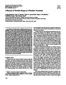
increases with decreasing mesh size. Note that, there is no formula to choose the value of the parameter α in the GHSS preconditioner. Its value is currently chosen on the basis of numerical tests. In the next sections we perform further numerical experiments to identify a strategy to select optimum value of the α. Further Analysis with α values for GHSS: Several values of α from 1.e − 4 to 1.e + 2 for GHSS have been used to solve the interface velocity
system preconditioned by GHSS. Values of α beyond the proposed range do not affect the results so we neglect them. In the following, we report some of the results of possible number of iterations of GHSS for the respective case of physical parameters. The best values of α for the respective parametric case are indicated. Number of iterations (Structured mesh, MINI ; P1 − P1 ) Grid ν = 10−4 , K = 10−3 ν = 10−6 , K = 10−5 ν = 10−6 , K = 10−8 1 2 3 4
ν = 100 , K = 100
4 (α = 1.e − 2)
2 (α = 1.e − 1)
1 (α = 1.e − 1)
4 (α = 1.e − 2)
5 (α = 1.e − 2)
2 (α = 1.e − 1)
1 (α = 1.e − 1)
11 (α = 1.e − 2)
5 (α = 1.e − 2)
2 (α = 1.e − 1)
7 (α = 1.e − 2)
3 (α = 1.e − 1)
1 (α = 1.e − 1) 1 (α = 1.e − 1)
8 (α = 1.e − 2)
10 (α = 1.e − 2)
We have presented the best values of α that should be used to get a number of iterations independent of mesh size. In figures 2.6 - 2.8 we plot the values of α that, corresponding to several values of K and ν, give the lowest number of iterations. The lines in the graphs represent the best-fitting curves. Unfortunately, a clear strategy as how to choose α has not been found yet. GHSS-like Preconditioners The GHSS preconditioner works well especially for low values of parameters. In this section, we consider some possible variants of the GHSS preconditioner with the aim of improving the previous results for physical parameters less than 1. GHSS-Variant(1) Preconditioning The preconditioner that we consider is similar in construction to the GHSS one, but two different values of α are used to characterize the preconditioner. Indeed, we have: P −1 = 2αd (Σd + αd I)−1 (Σs + αs I)−1
(2.77)
Numerical tests have been carried out for several values of αs and αd to characterise the best possible combination of both. (h1 h2 h3 h4 ) represents decreasing mesh sizes such that hj = 2−(j+1) .
2.6. Iteration Tests
38
ν = 10−4 2
y = − 0.05*x3 − 0.74*x2 − 4*x − 8.4 1
log10α
0
−1
−2
−3
−4 −8
−7
−6
−5
−4
−3
−2
log10K
Figure 2.6: Diamonds indicate the values of α that give the lowest number of iterations for the interface velocity system with GHSS preconditioner for different values of K and ν = 10−4
ν = 10−5 2
y = 0.012*x3 + 0.23*x2 + 0.55*x − 2.8 1
log10α
0
−1
−2
−3
−4 −8
−7
−6
−5
−4
−3
−2
log10K
Figure 2.7: Triangles indicate the values of α that give the lowest number of iterations for the interface velocity system with GHSS preconditioner for different values of K and ν = 10−5
2.6. Iteration Tests
39
ν = 10−6 2
y = 0.0031*x3 + 0.078*x2 − 0.079*x − 3.6 1
log10α
0
−1
−2
−3
−4 −8
−7
−6
−5
−4
−3
−2
log10K
Figure 2.8: Squares indicate the values of α that give the lowest number of iterations for the interface velocity system with GHSS preconditioner for different values of K and ν = 10−6 ν = 10−4 , K = 10−3
ν = 10−6 , K = 10−5
ν = 10−6 , K = 10−8
αd , αs
h1
h2
h3
h4
h1
h2
h3
h4
h1
h2
h3
h4
1.e − 3, 1.e − 2
4
4
4
5
2
2
2
2
1
1
1
1
2
3
3
3
1
1
2
2
1
1
1
1
1.e − 3, 1.e0
2
2
2
2
1
1
1
1
1
1
1
1
1
1
2
2
1
1
1
1
1
1
1
1
1.e − 3, 1.e + 2
1
1
1
1
1
1
1
1
1
1
1
1
2
2
2
3
1
1
1
1
1
1
1
1
1.e − 2, 1.e + 1
2
2
3
3
1
1
1
1
1
1
1
1
1.e − 2, 1.e + 4
1
1
1
1
1
1
1
1
1
1
1
1
2
3
4
6
1
1
1
1
1
1
1
1
1.e − 1, 1.e + 5
1
1
1
1
1
1
1
1
1
1
1
1
1.e − 3, 1.e − 1 1.e − 3, 1.e + 1 1.e − 2, 1.e + 2
1.e − 1, 1.e + 2
Iterations highlighted in bold identify possible optimal choices of αd and αs that lead to a number of iterations that does not depend on both h and the physical parameters. If we look at the construction of the preconditioner and at the numerical results, it looks that the Darcy operator Σd should dominate and Σs should be negligible if compared to I. Which implies for low αd and high αs . The other way round does not work for obtaining optimum results. This preconditioner can be used for any mesh size and low parametric values (less than 1) which is the case in most practical situations. The best possible combination can be αd = 1.e − 3, αs = 1.e + 2.
2.6. Iteration Tests
40
GHSS-Variant(2) Preconditioning For the GHSS-Variant(1) preconditioner, we obtained our best results for dominant Σd and negligible Σs as compared to I for low physical parameters. This consideration would lead to characterise another preconditioner which would involve only Σd as follows: P −1 = 2αd (Σd + αd I)−1
(2.78)
Numerical results for the solution of interface problem for velocity preconditioned by GHSSVariant(2) are presented here for several values of αd : ν = 10−4 , K = 10−3
ν = 10−6 , K = 10−5
ν = 10−6 , K = 10−8
αd
h1
h2
h3
h4
h1
h2
h3
h4
h1
h2
h3
h4
1.e − 1
4
5
7
10
2
3
3
3
2
2
2
2
1.e − 2
3
3
4
5
2
2
2
2
1
1
1
1
1.e − 3
2
3
3
3
2
2
2
2
1
1
1
1
1.e − 4
2
2
2
3
2
2
2
2
1
1
1
1
The GHSS-Variant(2) preconditioner has performed best so far. If used with αd = 1.e − 4 for the solution of the interface system, the iterative solver can converge in the same number of iterations irrespective of mesh size and almost of physical parameters as well. It gives solution with the least number of iterations with αd = 1.e − 4, for all cases of parametric values and mesh sizes.
Moreover, it is simpler than the GHSS and it can be solved using CG method that is cheaper than the GMRES. Neumann-Neumann Preconditioning In section 2.4.3 we introduced Neumann-Neumann preconditioner. These are characterized as −1 the sum of two operators (Σ−1 s and Σd ) weighted by the parameters θ1 and θ2 . The weighting
parameters are not known for this kind of problem. Having thorough numerical tests with DirichletNeumann and GHSS’s preconditioners we can propose the weighting parameters. It is already concluded for lower parameters that Σ−1 d should be dominant as the preconditioner like GHSS-I 1. Moreover, Σ−1 s should be dominant as the preconditioner for higher values of parameters. From this conclusion, we can propose following construction of the Neumann-Neumann preconditioner. P −1 = θs 2 (Σs )−1 + θd 2 (Σd )−1 where, θs =
νK νK+h
and θd =
h νK+h
(2.79)
with h being the mesh size.
It is clear in the construction of the preconditioner that for lower parameteric values weight θd2
2.7. Conclusion
41
would be higher as compared to θs2 so that Σ−1 d dominates. Similarly, for higher parameteric values −1 weight θs2 would be higher as compared to θd2 so that Σ−1 s dominates to Σd . Moreover, the con-
struction of the preconditioner is simple to operate. Also, it is symmetric-positive-definite so the preconditioned system can be solved by conjugate gradient method. In the following, we present the number of iterations of the CG method to solve the interface system of velocity preconditioned by Neumann-Neumann method.
mesh size h
ν = 10−4 , K = 10−3
ν = 10−6 , K = 10−5
ν = 10−6 , K = 10−8
ν = 1, K = 1
2−2
2
1
1
4
2−3
2
1
1
8
2−4
2
1
2
18
2−5
3
1
1
40
The results show that the Neumann-Neumann preconditioner for the interface system performs well for the all the parameters below 1. For unity parameters, the computational cost increases with the mesh refinement. If we change one of the weights like as follows, so that Darcy part doest not have any influence multiplied by a very low parameter as: P −1 = 2αθd 2 (Σd )−1 + θs 2 (Σs )−1 where, θd =
h νK+h
and θs =
iteration results:
νK νK+h
(2.80)
with h as the mesh size and α = 1.e − 4, we have the following
mesh size h
ν = 10−4 , K = 10−3
ν = 10−6 , K = 10−5
ν = 10−6 , K = 10−8
ν = 1, K = 1
2−2
3
2
1
4
2−3
3
2
1
5
2−4
3
2
1
5
2−5
4
2
2
5
We can reckon that for higher physical parameters, Dirichlet-Neumann preconditioner should be used for the interface system. And for low physical parameters Neumann-Neumann precondition (2.79) should be operated for the system. Most of the practical applications involve low physical parameters.
2.7
Conclusion
In this chapter, we studied the numerical solution of the steady state Stokes-Darcy coupled problem. Effective solution methods have been proposed.
2.7. Conclusion
42
We have presented the weak-formulation of the coupled Stokes-Darcy problem. A primal mixed formulation for Darcy has been used in variational formulation. This approach naturally allows to impose the interface conditions. The weak formulation has been discretised using finite elements. Having discretised the weak form, the algebraic form of the coupled problem has been obtained. For general practical problem the linear system would be large so an objective is to propose a cheaper and effective method of solution. The method of Schur complements has been used to reduce the large system to the interface problem for velocity and pressure. In this way, a smaller system is solved for the variables at the interface and quantities in domains are solved with the help of Schur complements. This approach is cheaper than solving the large system. The Schur complement system is expensive to solve and the number of iterations for the solution to converge increases with the mesh refinement and depend on the physical parameters as well. We have proposed the use of preconditioned systems which should work with the same cost for the problem of any nature. We propose Neumann-Neumann preconditioner of the form; −1 P −1 = θ1 Σ−1 s + θ2 Σd
(2.81)
This kind of preconditioner has advantages over others. It is simple to operate because of addition of two operators. The operators can be computed in parallel then used. Also strategies to compute weights are available. We propose here that the weights could be chosen as in (2.79) when the physical parameters are low. When the physical parameters are higher, then only the Stokes part should be used by setting the weights as θ1 = 1; θ2 = 0. This proposed method allows to solve the coupled problem in the most general efficient and cheaper way.
Chapter 3
Unsteady Stokes-Darcy Problem In the unsteady case we will have the complete general form of the coupled Stokes-Darcy problem. Now, all the quantities are functions of space as well as of time. ∂us − ν△us + ∇ps = f ∂t ∇ · us = 0
in Ωs
(3.1)
in Ωs
(3.2)
uD s
on ∂Ωs,D
(3.3)
ν∇us · n − ps n = φN
on ∂Ωs,N
(3.4)
in Ωd
(3.5)
us =
ud = −K∇pd
So
∂pd + ∇ · ud = f d ∂t pd = pD d
in Ωd
(3.6)
on ∂Ωd,D
(3.7)
uN d
on ∂Ωd,N
(3.8)
on Γ
(3.9)
ud · n =
us · n = ud · n,
∂us + ps = gpd ∂n ∂us ν −ντ j · = us · τ j ∂n ǫ
−νn ·
on Γ (j = 1, . . . , n − 1)
(3.10) on Γ.
(3.11)
At initial time t = t0 ; us , ps , ud and pd are defined.
3.1
Weak Formulation
We will follow the same approach as we did in the weak formulation of the steady case. Th only difference would be the addition of new term of time increment. We have the following weak
3.2. Finite Element Approximation in Space
44
formulation of the problem using the same procedure and notations.
3.1.1
Z Z
Ωs
Stokes
∂u0s ·vs + ∂t
Z
Ωs
j=1
Z n−1 Z Xν ∂uD s D D φN vs ν∇us · ∇vs − · vs − (u · τ j )(vs · τ j ) + ∂t ǫ s Γ Ωs ∂Ωs,N Z
Ωs
j=1
−
3.1.2
Z
Ωd
3.2
Z
Ωs
∇ · u0s qs =
Z
Ωs
∇ · uD s qs
∀ vs ∈ H 1∂Ωs ,D (Ωs ) (3.12)
∀qs ∈ L2 (Ωs )
(3.13)
Darcy 1 2
1 2
Z n−1 Z Xν 0 ps ∇·vs + gpd (vs ·n)+ f ·vs − (u ·τ j )(vs ·τ j ) = ǫ s Γ Γ Ωs Ωs Z
Z
ν∇u0s ·∇vs −
Z
K
−1
Ωd
1 gud · vd + 2
Z
Ωd
g∇p0d
1 · vd = − 2
Z
Ωd
g∇pD d · vd
∀vd ∈ L2 (Ωd )
(3.14)
Z Z Z ∂p0d 1 g(uN ·qd − (Kg∇p0d ·∇qd ) = − gfd qd + d )qd ∂t 2 Ωd ∂Ωd,N Γ Ω Ωd Z Z Z ∂pD 1 1 D d (Ωd ) (3.15) gSo ∀qd ∈ H∂Ω (Kg∇pD · qd + − g(us · n)qd + d · ∇qd ) d ,D ∂t 2 Ωd Ωd Γ
gud ·∇qd +
Z
g(u0s ·n)qd −
Z
gSo
Finite Element Approximation in Space
The finite elements for the coupled Stokes-Darcy problem has already been discussed in steady case; see section 2.2. We will use the same finite element setting in space for time-dependent problem. We define the following basis for the Finite Element discretization. In terms of shape functions we can write; us =
nsu X j=1
ujs Njsu ,
ps =
nsp X
j , pjs Nsp
vs = Nisu
i = 1 . . . nsu
and
i qs = Nsp
i = 1 . . . nsp
j=1
where, Nsu and Nsp are the shape functions of the Stokes velocity and Stokes pressure fields respectively. Moreover, nsu is the number of internal nodes for Stokes Velocity with interface included and nsp are the number of all nodes for Stokes pressure. We will indicate number of velocity nodes on interface by nsΓ , dirichlet nodes on boundaries by nsu,D and dirichlet nodes on
3.2. Finite Element Approximation in Space
45
interface by nsΓ,D . Similarly, ud =
ndu X
ujd Njdu ,
pd =
j=1
ndp X
j pjd Ndp ,
vd = Nidu
i = 1 . . . ndu
and
i qd = Ndp
i = 1 . . . ndp
j=1
where, Ndu and Ndp are the shape functions of the velocity and pressure fields respectively in porous medium. Moreover, ndu are the number of all nodes for Darcy velocity excluding Neumann boundary and ndp are the number of nodes for Darcy pressure fields with interface included. We will indicate number of pressure nodes on interface by ndΓ , dirichlet nodes by ndp,D .
Stokes Now, (3.12) and (3.13) can be written in discrete form as; Z
nsu X ∂u0,j s
∂t
Ωs j=1
+
Z X ndΓ Γ j=1
−
Z
+
Z
Njsu
j gpjd Ndp (Nisu
+
Z
ν
Ωs
nsu −nsΓ X j=1
∂uD,j s
Ωs j=1
∂t
Njsu · Nisu −
φN Nisu
j u0,j s ∇Nsu
·
∇Nisu
−
Z
nsp X
Ωs j=1
j pjs Nsp ∇ · Nisu
Z n−1 Z nsΓ Xν X 0,j j i · n) + f · Nisu ( us Nsu · τ k )(Nsu · τ k ) = ǫ Γ Ωs k=1
nsu X
∂Ωs,N
· Nisu
Z
j=1 nsu,D
ν Ωs
X j=1
j i uD,j s ∇Nsu · ∇Nsu −
nsΓ,D Z X n−1 ν X D,j j ( us Nsu · τ k )(Nisu · τ k ) ǫ Γ j=1
k=1
for every internal velocity node i
(3.16)
and −
Z
nsu X
Ωs j=1
u0,j s ∇
·
i Njsu Nsp
=
Z
nsu,D
X
j i uD,j s ∇ · Nsu Nsp
Ωs j=1
for every pressure head node i (3.17)
Darcy Descretisation of the (3.14) and (3.15) is as follows; 1 2
Z
K Ωd
−1
g
ndu X j=1
ujd Njdu
·
Nidu
1 + 2
Z
Ωd
g
ndp X j=1
j p0,j d ∇Ndp
· Nidu
1 =− 2
Z
Ωd
ndp,D
g
X j=1
j i pD,j d ∇Ndp · Ndu
for every velocity node i
(3.18)
3.3. Time Discretisation 1 2
Z
g Ωd
1 − 2
3.3
ndu X
ujd Njdu
j=1
Z
(Kg
Ωd
−
Z
+
1 2
46
j=1
nsΓ,D
g(
Γ
ndp X
X
j p0,j d ∇Ndp
j uD,j s Nsu
j=1
Z
Ωd
(Kg
·
i ∇Ndp
·
+
Z
Γ
·
Z nsΓ X 0,j j i g( us Nsu · n)Ndp − j=1
i ) ∇Ndp
i n)Ndp
+
Z
=−
gSo Ωd
ndp,D
X j=1
Z
j i pD,j d ∇Ndp · ∇Ndp )
Ω
i gfd Ndp
ndp X ∂pD,j d
j=1
∂t
+
Z
gSo Ωd
∂Ωd,N
ndp X ∂p0,j d
j=1
∂t
j i Ndp · Ndp
i g(uN d )Ndp
j i Ndp · Ndp
for every internal pressure node i
(3.19)
Time Discretisation
Now, We discretise the form (3.16) - (3.19) in time. The Backward Euler Difference Scheme will be used for approximation in time. This algorithm is stable unconditionally and accurate in first order. Let the [0, T ] be the period of time of the problem. Divide the interval [0, T ] into N subintervals [tm , tm+1 ], (m = 0, 1, 2...N ) satisfying 0 = t0 < t1 < ... < tN −1 < tN = T Let ∆t = tm+1 − tm then for any problem point in time is
∂x = f the Backward Euler approximation at the tm+1 ∂t
xm+1 − xm xm+1 xm = f m+1 =⇒ = f m+1 + ∆t ∆t ∆t
where, for every function X; X m = X(tm ). So, the BEDS for the semi-discretised coupled Stokes-Darcy problem (3.16) - (3.19) for any point tm+1 in time is as follows;
3.3. Time Discretisation
47
Stokes
Z
nsu 0,j,m+1 X us − u0,j,m s
∆t
Ωs j=1
+
Z X ndΓ Γ j=1
−
· Nisu
Z
+
ν
Ωs
nsu −nsΓ X j=1
u0,j,m+1 ∇Njsu s
·
∇Nisu
−
nsp X
Z
Ωs j=1
j pj,m+1 Nsp ∇ · Nisu s
Z n−1 Z nsΓ Xν X j,m+1 j i 0,j,m+1 j i gpd Ndp (Nsu · n) + f m+1 · Nisu ( us Nsu · τ k )(Nsu · τ k ) = ǫ Γ Ωs
Ωs j=1
j=1
k=1
nsu X
Z
Njsu
uD,j,m+1 − uD,j,m s s Njsu · Nisu − ∆t
nsu,D
Z
X
ν
Ωs
j=1
uD,j,m+1 ∇Njsu s
·
∇Nisu
+
Z
m+1
∂Ωs,N
φN Nisu
Z n−1 sΓ,D X ν nX − ( uD,j,m+1 Njsu · τ k )(Nisu · τ k ) for every internal velocity node i s ǫ Γ
(3.20)
j=1
k=1
and −
nsu X
Z
Ωs j=1
u0,j,m+1 ∇ s
·
i Njsu Nsp
=
nsu,D
Z
X
Ωs j=1
i uD,j,m+1 ∇ · Njsu Nsp s
for every pressure node i (3.21)
Darcy
1 2
Z
−
1 2
1 2
Z
−
1 2
K
−1
g
Ωd
Z
Z
g Ωd
+
1 2
X j=1
ndu X
1 + 2
Z
g Ωd
j pD,j,m+1 ∇Ndp · Nidu d
uj,m+1 Njdu d
j=1
(Kg Ωd
g(
Γ
X j=1
(Kg Ωd
i · ∇Ndp
+
Z
Γ
ndp
X j=1
nsΓ,D
Z
· Nidu
ndp,D
Ωd
−
uj,m+1 Njdu d
j=1
g Z
ndu X
ndp,D
X j=1
j=1
j p0,j,m+1 ∇Ndp · Nidu = d
for every velocity node i Z nsΓ X 0,j,m+1 j i g( us Nsu · n)Ndp − j=1
j i p0,j,m+1 ∇Ndp · ∇Ndp )=− d
i uD,j,m+1 Njsu · n)Ndp + s
ndp X
Z
Ωd
Z
Ω
i gfdm+1 Ndp +
Z
(3.22)
gSo Ωd
∂Ωd,N
ndp 0,j,m+1 X p − p0,j,m d
j=1
d
∆t
j i Ndp · Ndp
i g(uN,m+1 )Ndp d
ndp
gSo
X pD,j,m+1 − pD,j,m d
j=1
d
∆t
j i Ndp · Ndp
j i pD,j,m+1 ∇Ndp · ∇Ndp )for every internal pressure head node i d
(3.23)
3.4. Algebraic Formulation
3.4
48
Algebraic Formulation
We have the discrete equations (3.20) and (3.21) for Stokes and (3.22) and (3.23) for Darcy. Now, we will proceed to the Algebraic formulations of the coupled problem. We introduce the following matrices and column-matrices;
Z
(Msu )ij =
nsu X
Ωs j=1
Z
I
(A1 )ij =
i = 1, . . . nsu , j = 1, . . . nsu
ν∇Nisu · ∇Njsu
Ωs Z n−1 X
(A1 Γ )ij =
Njsu · Nisu
Γ
i = 1, . . . nsu , j = 1, . . . nsu − nsΓ
ν i (N · τ k )(Njsu · τ k ) ǫ su
i = 1, . . . nsu , j = 1, . . . nsΓ
Z k=1 i ∇ · Nsu Njsp i = 1, . . . nsu , j = 1, . . . nsp (B1 )ij = − Z Ωs j g(Nisu · n)Ndp i = 1, . . . nsu , j = 1, . . . ndΓ (PΓ )ij =
A1 = A1 I + A1 Γ
Γ
(F 1 )i =
Z
Ωs
f m+1 · Nisu −
nsΓ,D
−
Z
Ωs
nsu,D
ν
X j=1
uD,j,m+1 ∇Njsu · ∇Nisu − s
Z
Ωs j=1
Z Z n−1 Xν X j i Nisu φm+1 ( uD,j,m+1 N · τ )(N · τ ) + k k s su su N ǫ ∂Ωs,N Γ k=1
(F12 )i =
Z
j=1 nsu,D
X
Ωs j=1
i uD,j,m+1 ∇ · Njsu Nsp s
i = 1, . . . nsp
nsu D,j,m+1 X us − uD,j,m s
∆t
i = 1, . . . nsu
Njsu · Nisu
3.4. Algebraic Formulation
49
1 (A2 )ij = 2
Z
K −1 gNjdu · Nidu
1 (B2 )ij = 2
Z
g
Ωd
Ωd
(Mdp )ij = −
Z
(F 21 )i = −
1 2
(F2 )i = − +
Z
Ωd
j ∇Ndp · Nidu
gSo
ndp X
Ωd
1 2
(S)ij = −
ndp X j=1
Z
Z
Z
Ω
j=1 ndp
(Kg
Ωd
i = 1, . . . ndu , j = 1, . . . ndu
X
j=1 ndp,D
i = 1, . . . ndu , j = 1, . . . ndp
j i Ndp · Ndp
i = 1, . . . ndp , j = 1, . . . ndp
j i p0,j d ∇Ndp · ∇Ndp ) i = 1, . . . ndp , j = 1, . . . ndp
j pD,j,m+1 ∇Ndp · Nidu d
X
Ωd j=1
i gfdm+1 Ndp
+
Z
i = 1, . . . ndu
i g(uN d )Ndp
j i + Ndp · Ndp
∂Ωd,N
ndp
gSo
X pD,j,m+1 − pD,j,m d
d
∆t
j=1
nsΓ,D
−
Z
g(
1 2
Z
(Kg
Γ
X
i uD,j,m+1 Njsu · n)Ndp s
j=1 ndp,D
Ωd
X j=1
j i ) pD,j,m+1 ∇Ndp · ∇Ndp d
i = 1, . . . ndp
The discrete equations can be written in the algebraic form as follows;
1 ∆t Msu + B1T
A1 B1
0
PΓ
0
0
0
0
0
A2
B2
PΓT
0
B2T
1 ∆t Mdp
+S
u ˜m+1 s
m+1 p˜s = u m+1 ˜d p˜m+1 d
F1 +
1 ˜m s ∆t Msu u
F12 F 21 F2 +
1 ˜m d ∆t Mdp p
(3.24)
Referring to above system, u ˜m+1 is the vector of values of u0s on all internal velocity nodes of s and p˜m+1 are the vectors of the pressure and pressurethe Stokes domain at time tm+1 . p˜m+1 s d head values respectively, on all pressure nodes of Stokes and Darcy domain respectively at time tm+1 . Similarly, u ˜m+1 is the vector of all values of ud on the velocity nodes in the Darcy domain d computed for time tm+1 . Writing AM 1 = and F2M = F2 +
1 ˜m d ∆t Mdp p
1 ∆t Msu
+ A1 , S M =
1 ∆t Mdp
+ S, F M 1 = F1 +
1 ˜m s ∆t Msu u
then; AM 1T B1 0 PΓT
B1
0
0 0
0 A2
0
B2T
PΓ
u ˜m+1 s
FM 1
m+1 0 p˜s = F12 m+1 B2 u ˜d F 21
SM
p˜m+1 d
F2M
(3.25)
3.4. Algebraic Formulation
50
Putting in evidence the interface values, we get:
AM 1,ii
AM 1,iΓ
B1i
0
0
0
m+1 u˜i s
FM 1i
m+1 M PΓ uΓ F 1Γ 0 p˜m+1 F12 s = m+1 ˜d F 21 B2Γ u M M ˜i m+1 SiΓ p d F2 M M SΓΓ F2Γ pm+1 Γ
M A1,Γi AM 0 0 1,ΓΓ B1Γ BT T B1Γ 0 0 0 1i 0 0 0 A2 B2i 0 T 0 0 B2i SiiM T M 0 PΓT 0 B2Γ SΓi
(3.26)
uΓ is the vector of nodal values of the normal velocity at the interface Γ and pΓ is the nodal values of the pressure head at the interface Γ. If we condense the Stokes variables u˜i and p˜ into one s
s
variable us then the resulting algebraic system can be written as;
As
BsΓ
0
0
T 0 0 BsΓ AM 1,ΓΓ 0 0 A2 B2i T 0 B2i SiiM 0 T M 0 PΓT B2Γ SΓi
m+1 us Fs m+1 M uΓ PΓ F 1Γ m+1 u ˜d = B2Γ F 21 m+1 M M ˜ i SiΓ F p d 2 M M SΓΓ F2Γ pm+1 Γ 0
(3.27)
If we also condense the Darcy variables u ˜d and p˜i d into one variable ud then the resulting algebraic system can be written as; As BsΓ 0 0 um+1 Fs s m+1 M T BsΓ AM 0 PΓ 1,ΓΓ uΓ = F 1Γ 0 m+1 0 Ad BdΓ ud F d M T M SΓΓ 0 PΓT BdΓ pm+1 F2Γ Γ
(3.28)
um+1 , um+1 are the quantities in the interior of the domains excluding the interface Γ computed s d at time tm+1 . The coefficient matrix of the above linear system (3.28) is generally large, sparse, M is negative diagonal symmetric and indefinite; having both positive and negative eigenvalues (SΓΓ matrix). The coupling between the Stokes and mixed formulated Darcy Equations are realised by
the second and fourth rows of the system. Notice that, the sub-matrices PΓ and PΓT impose the algebraic counterpart of the coupling conditions. Above system is similar in construction to the system for steady case. We will proceed now to more simplified form using Shur complements.
3.4.1
Schur Complement Systems
We will find the Schur complements systems with respect to the normal velocity and pressure head on the interface. The variables for internal domains are eliminated and system is solved for the interface variables. Same procedure would be followed as done for the steady case. Following are
3.5. Solution Methods
51
the linear systems for the interface velocity and pressure head on interface for time tm+1 . = f 1Γ − PΓ Σ−1 (Σs + Σd ) um+1 c f2Γ Γ
(3.29)
= f2Γ − PΓT Σ−1 (Σc + Σf ) pm+1 s f 1Γ Γ
(3.30)
T −1 Σs = (AM 1,ΓΓ − BsΓ As BsΓ )
(3.31)
where,
Σc =
M (SΓΓ
Σd =
T −PΓ Σ−1 c PΓ
Σf
−
T BdΓ A−1 d BdΓ )
= −PΓT Σ−1 s PΓ
T −1 f 1Γ = F M 1Γ − BsΓ As F s M T A−1 f2Γ = F2Γ − BdΓ d Fd
(3.32) (3.33) (3.34) (3.35) (3.36)
The above system is solved for every subinterval of time for the interface quantities. Once the interface quantities are solved, these are used for the quantities on the interior of domains with the help of Schur complements.
3.5
Solution Methods
We have the large systems (3.29) and (3.30) for the velocity and pressure head on interface at any discrete point of time. These systems are solved for every subintervals of the total time period. In general, these systems are large and ill-conditioned which make them computationally very expensive. As we have already seen the solution methods in steady case, same approach would be used for unsteady case as well. The systems in this unsteady case are similar to that for steady case. Here, the Krylov subspace methods will be used such that Conjugate gradient and GMRES which have already been discussed in previous chapter.
3.5.1
Preconditioning
As discussed in section 2.4.3, preconditioning is an effective way of reducing the computational cost and make it independent of mesh refinement. Here, we will present preconditioners that can be operated on the interface problems for velocity and pressure head. The systems are similar to that for the time-independent problem. So, same types of preconditioners can be used here as well; Domain Decomposition Methods As the system is composed of two parts, we can get preconditioners from the Domain decomposition method as follows.
3.6. Numerical Tests and Analysis
52
• Dirichlet-Neumann P1−1 = Σ−1 s
for (3.29)
(3.37)
P2−1 = Σ−1 c
for (3.30)
(3.38)
• Neumann-Neumann −1 P1−1 = θ1 Σ−1 s + θ2 Σd
for (3.29)
(3.39)
−1 P2−1 = θ1 Σ−1 c + θ2 Σf
for (3.30)
(3.40)
where θ1 and θ2 are suitable weights which should be defined specifically for the problem. As these preconditioners are symmetric and these will result the symmetric systems from the original systems so conjugate gradient iterative solver would be operated to solve the interface systems preconditioned by the above operators. GHSS Method From Benzi [Ben09], We can use GHSS method to split the above matrix systems and we follow the similar approach as we used for the steady case, as the systems are similar. By this approach coefficient matrix is split into three parts say A = (G + K) + S; for our case S can be taken as zero and coefficient matrices are of the form A = G + K. Following the approach, in (3.29) and (3.30), the coefficient matrices are already composed of two positive definite parts. So by GHSS the Preconditioners are characterised as; � �� � P1 = (2α2 )−1 Σs + α2 I Σd + α2 I � �� � P2 = (2α3 )−1 Σc + α3 I Σf + α3 I
for (3.29)
(3.41)
for (3.30)
(3.42)
Σs and Σc matrices are symmetric having the factor of kinematic viscosity (ν), Darcy conductivity (K) and storativity (S) which are usually small in most of the practical applications. These preconditioners are non-symmetric and it can be easily seen that these will result the non-symmetric matrices if used with the original systems. So, the resulted systems are solved by GMRES iterative solver.
3.6
Numerical Tests and Analysis
A matlab code to solve the Steady coupled Stokes-Darcy problem is extended for the unsteady problem. With the help of numerical tests we will analyse the convergence of the coupled problem and the performance of preconditioners.
3.6. Numerical Tests and Analysis
53
For the numerical tests we consider a time interval [0, T ]. The time interval is dicretised into N subintervals each with the duration of ∆t. The problem is solved in space for each subinterval until the final time T is reached. The initial value of the quantities at t = t0 (= 0) are given. Moreover, We consider a computational domain; Ω ⊂ R2 composed of two sub-domains Stokes Ωs = (0, 1) × (1, 2)
and Darcy Ωd = (0, 1) × (0, 1). The sub-domains are separated by the interface Γ = (0, 1) × {1}.
Domains Ωs and Ωd have boundaries ∂Ωs = ∂Ωs,D ∪ ∂Ωs,N and ∂Ωd = ∂Ωd,D ∪ ∂Ωd,N respectively where we can impose dirichlet and Neumann boundary conditions of the problem. MINI and Taylor-
Hood finite elements are used for Stokes domain and standard elements P1 − P1 and P1 − P2 for Darcy domain. Similar to steady problem, The 2D setting considered here has interface Γ parallel ∂Ωs,D
∂Ωs,D
Ωs
∂Ωs,N
Γ
∂Ωd,N
Ωd
∂Ωd,N
∂Ωd,D
Figure 3.1: Computational domain for numerical tests
to the x-axis, so that orthogonal normal and tangential unit vectors are n = (0, −1) and τ = (1, 0)
respectively. We will focus on the interface problem for velocity (3.29) only.
3.6.1
Error Convergence of the Solution
We present the convergence of the numerical solution towards a known exact one as the grid size reduces. The initial values, boundary conditions and forcing terms are chosen in such a way that exact solution of the coupled Stokes-Darcy problem for the computational domain 3.1 is (us1 , us2 ) = (ey cos(2πt), −ex cos(y)cos(2πt)) ps = ex sin(y)cos(2πt)
(ud1 , ud2 ) = (−ex sin(y)cos(2πt), −ex cos(y)cos(2πt)) pd = ex sin(y)cos(2πt)
(3.43) (3.44) (3.45) (3.46)
3.6. Numerical Tests and Analysis
54
We will check the convergence of the L2 and H 1 norms of the errors of the approximated solution as compared to the given exact solution at the given time t. Following are the rates of error norms as the grid is refined such that for grid index j, the grid size is 2−(j+1) units and time interval ∆t is reduced in relation to grid size. Following are the results for the domain discretised into first order finite elements that are M IN I for Stokes and P1 − P1 for Darcy domain with different order contributions of h and ∆t. Numerical Results with ∆t = h2 The following table summarizes errors for solution of the interface problem for velocity with ∆t = h2 at T = 1s. ||uf − uhf ||0
||uf − uhf ||1
|uf − uhf |1
||div(uf − uhf )||0
||pf − phf ||0
2−6
0.041388
0.222736
0.218857
0.049796
0.590352
2−8
0.010660
0.090958
0.090331
0.022602
0.147570
Grid; h
∆t
1; 2−2
2−4
||ud − uhd ||0
||div(ud − uhd )||0
||pd − phd ||0
||pd − phd ||1
|pd − phd |1
2;
2−3
2−6
0.049076
0.546321
0.020229
0.127484
0.125868
3;
2−4
2−8
0.013658
0.363463
0.0052003
0.061043
0.060821
Grid; h
∆t
1; 2−2
2−4
2;
2−3
3;
2−4
Stokes
Darcy
0.147224
0.168147
0.633834
0.847967
0.616498
0.155205
0.073042
0.282884
2.350706
0.273292
Convergence Rates with ∆t = h2 Following table shows the convergence rates of the interface problem for velocity with ∆t = h2 at T = 1s: • Stokes Problem (Structured mesh of M IN I elements) Grid; h ∆t ||uf − uhf ||0 ||uf − uhf ||1 |uf − uhf |1
||div(uf − uhf )||0
||pf − phf ||0
1; 2−2
2−4
-
-
-
2;
2−3
2−6
1.830736
1.508770
1.494109
1.640065
1.993445
3;
2−4
2−8
1.9569708
1.292054
1.276684
1.139578
2.000170
• Darcy Problem (Structured mesh of P1 − P1 elements) Grid; h ∆t ||ud − uhd ||0 ||div(ud − uhd )||0 ||pd − phd ||0 1; 2−2 2; 2−3
2−4 2−6
1.776632
0.6342608
1.852276
3; 2−4
2−8
1.845245
0.587939
1.959776
-
-
||pd − phd ||1
|pd − phd |1
1.062417
1.049276
1.149895
1.118521
As, we can see that errors decrease with the reduction of the mesh size and time interval. From the above results for h reducing by factor of half and ∆t = h2 , it is clear that L2 norm of error of
3.6. Numerical Tests and Analysis
55
velocity in Stokes domain converges with the rate of about 2. Same result is shown for the velocity in Darcy domain. H 1 norm of the error of the Stokes velocity decreases with the rate of about 1.5 while these norms for Darcy pressure are even less as 1.1. L2 norm of the error of the divergence of the Stokes velocity has convergence rate of less than 1.5 while that for Darcy velocity is 0.6. Numerical Results with ∆t = h3 The following table summarizes errors for solution of the interface problem for velocity with ∆t = h3 at T = 1s. Stokes
Darcy
||uf − uhf ||0
||uf − uhf ||1
|uf − uhf |1
||div(uf − uhf )||0
||pf − phf ||0
2−9
0.007468
0.166311
0.166143
0.044365
0.089211
Grid; h
∆t
1; 2−2
2−6
||ud − uhd ||0
||div(ud − uhd )||0
||pd − phd ||0
||pd − phd ||1
|pd − phd |1
2−3
2−9
0.024392
0.552331
0.003183
0.119867
0.119825
Grid; h
∆t
1; 2−2
2−6
2; 2−3
2;
0.043376
0.085037
0.361938
0.841641
0.359330
0.020617
0.096739
0.239846
0.643251
0.238958
Convergence Rates with ∆t = h3 at T = 1s. Here, we will present some of the convergence rates of the interface problem for velocity with ∆t = h2 at T = 1s. • Stokes Problem (Structured mesh with M IN I elements) Grid; h ∆t ||uf − uhf ||0 ||uf − uhf ||1 |uf − uhf |1 ||div(uf − uhf )||0 1; 2−2
2−6
-
-
-
-
2; 2−3
2−9
2.538026
1.121861
1.112882
1.124665
• Darcy Problem (Structured mesh of P1 − P1 elements) Grid; h ∆t ||ud − uhd ||0 ||div(ud − uhd )||0 ||pd − phd ||0 1; 2−2
2−6
-
-
-
2; 2−3
2−9
1.801680
0.607671
2.695159
||pf − phf ||0 -
2.850081
||pd − phd ||1
|pd − phd |1
1.000668
0.995827
-
-
The tables above summarise the errors and convergence of the errors for the h reducing by half and ∆t = h3 . It is clear from the results that L2 norm of the error of Stokes velocity converge with the rate of about 2.5 and that of Darcy velocity with rate of 1.8. L2 norm of error of pressure in Stokes and Darcy converge with the improved rate of above 2.5.
3.7. Numerical Tests for Iterations
3.7
56
Numerical Tests for Iterations
Now, we will discuss the behaviour of iterative methods and their computational cost depending on the mesh refinement, time interval and physical parameters. As stated before, interface systems (3.29) and (3.30) are solved by the effective iterative methods CG or GMRES. The linear system for interface velocity is solved here with various mesh size such that for grid index j the grid size is 2−(j+1) . For the following numerical results; the initial values, boundary conditions and forcing terms are chosen in such a way that exact solution of the coupled Stokes-Darcy problem for computational domain (figure 3.1) is
(us1 , us2 ) = (((y − 1)2 + (y − 1) + ǫ)cos(2πt), x(x − 1)cos(2πt)), (ǫ = 1) ps = 2ν(x + y − 1)cos(2πt),
(3.48)
(ud1 , ud2 ) = (((2x − 1)(y − 1) − 2ν)cos(2πt), ((x2 − x) − (y − 1)2 )cos(2πt)), pd = ((1/K)(x(1 − x)(y − 1) + (1/3)(y − 1)3 ) + 2νx)cos(2πt)
3.7.1
(3.47)
(3.49) (3.50)
Non-Preconditioned
First we will solve the interface system for velocity without the preconditioning. The system is solved by the conjugate gradient method. Following are the iterations for the solution of the problem for different cases of the problem. Number of Iterations for ∆t = 0.5 (Structured Mesh with MINI ; P1 − P1 elements) Grid ν = 10−4 , K = 10−3
ν = 10−6 , K = 10−5
ν = 10−6 , K = 10−8
ν = 100 , K = 100
1
4
4
4
4
2
9
9
10
8
3
20
20
24
16
4
34
34
39
28
Number of Iterations for ∆t = 0.01 (Structured Mesh with MINI ; P1 − P1 elements) Grid ν = 10−4 , K = 10−3 ν = 10−6 , K = 10−5 ν = 10−6 , K = 10−8 ν = 100 , K = 100 1
4
4
4
4
2
9
9
10
8
3 4
20 33
20 35
24 39
14 21
As we can see from the above results that computational cost increases with the mesh refinement. When the physical parameters are low, the system takes more iterations before converging to the solution. Now, we proceed to the preconditioned system to make the solution independent
3.7. Numerical Tests for Iterations
57
of the mesh refinement and physical nature.
3.7.2
Preconditioned
Preconditioning for the linear system of the coupled problem is already discussed in the section 3.5.1. We will analyse the iterations of the solver to solve the linear system for the interface velocity within the given tolerance of 10−9 . Dirichlet-Neumann preconditioner will be used first of all then the GHSS and the Neumann-Neumann at the end. 1. Dirichlet-Neumann P −1 = Σ−1 s
(3.51)
This is the simplest operator for preconditioning. As it is the symmetric-positive-definite and the preconditioned system would also be SPD, so conjugate gradient method can be operated for the solution. Following are the iteration results for the linear system of interface velocity solved by CG preconditioned by the Dirichlet-Neumann operator. Number of Iterations for ∆t = 0.5 (Structured Mesh with MINI ; P1 − P1 elements) Grid ν = 10−4 , K = 10−3 ν = 10−6 , K = 10−5 ν = 10−6 , K = 10−8 ν = 100 , K = 100 1
4
4
4
4
2
8
8
9
5
3
16
14
14
5
4
19
14
13
5
Number of Iterations for ∆t = 0.01 (Structured Mesh with MINI ; P1 − P1 elements) Grid ν = 10−4 , K = 10−3 ν = 10−6 , K = 10−5 ν = 10−6 , K = 10−8 ν = 100 , K = 100 1
4
4
4
4
2
9
9
8
4
3
14
14
13
4
4
13
13
13
4
The results show the iteration tests for varying mesh size and for two different time step sizes. The computational cost increases as the mesh is refined except for the case of unity physical parameters. This preconditioner has improved the results for the case of the higher values of physical parameters. For this case, same number of iterations are required independent of mesh size. To some extent, the system for small time step size is easier to solve. We should proceed to other preconditioners.
3.7. Numerical Tests for Iterations
58
2. GHSS P −1 = 2α(Σd + αI)−1 (Σs + αI)−1
(3.52)
Dirichlet-Neumann is useful when the physical parameters have higher values. Here, we will test the GHSS preconditioner. This is difficult to operate because of its composition. This operator is not symmetric in general so the system preconditioned by this operator would not be symmetric. Therefore, GMRES solver is used for the solution of the interface sytem preconditioned by GHSS. Number of Iterations for ∆t = 0.5 (Structured Mesh with MINI ; P1 − P1 elements); α = 1e − 3
Grid
ν = 10−4 , K = 10−3
ν = 10−6 , K = 10−5
ν = 10−6 , K = 10−8
ν = 100 , K = 100
1
4
4
4
4
2
8
8
8
8
3
16
16
16
16
4
27
32
30
21
First, we have used the general value of the parameter α in the GHSS preconditioner. For this case, the iteration results are not optimum and these are even worse than those for the Dirichlet-Neumann. As value of α is not fixed, we can test several values of α and find the best value for each case of physical prametric values. Having done rigorous numerical tests, following are the results for different cases of physical values with corresponding to the best value of α.
Number of Iterations for ∆t = 0.5 (Structured Mesh with MINI ; P1 − P1 elements) Grid
ν = 10−4 , K = 10−3
ν = 10−6 , K = 10−5
ν = 10−6 , K = 10−8
ν = 100 , K = 100
1
4 (α = 1.e − 1)
4 (α = 1.e0)
2 (α = 1.e0)
4 (α = 1.e0)
2 (α = 1.e0)
4 (α = 1.e − 1)
4 (α = 1.e0) 4 (α = 1.e0)
2 (α = 1.e0) 2 (α = 1.e0)
2 3 4
7 (α = 1.e − 1)
8 (α = 1.e − 1) 13 (α = 1.e − 1)
7 (α = 1.e − 1)
8 (α = 1.e − 1) 8 (α = 1.e − 1)
The above results show the improved performance of the GHSS operator unless good α value is chosen for every case of physical nature of the problem. This preconditioner has performed very well specifically when the physical parameters have low values. Number of Iterations for ∆t = 0.01 (Structured Mesh with MINI ; P1 − P1 elements) α = 1e − 3 Grid
ν = 10−4 , K = 10−3
ν = 10−6 , K = 10−5
ν = 10−6 , K = 10−8
ν = 100 , K = 100
1
4
4
1
4
2
8
8
1
8
3
16
16
3
16
4
32
32
8
21
3.7. Numerical Tests for Iterations
59
Number of Iterations for ∆t = 0.01 (Structured Mesh with MINI ; P1 − P1 elements) Grid
ν = 10−4 , K = 10−3
ν = 10−6 , K = 10−5
ν = 10−6 , K = 10−8
ν = 100 , K = 100
1
4 (α = 1.e − 1)
4 (α = 1.e0)
4 (α = 1.e0)
8 (α = 1.e0)
7 (α = 1.e0)
4 (α = 1.e − 1)
9 (α = 1.e0)
7 (α = 1.e0)
4 (α = 1.e0)
6 (α = 1.e0)
2 3 4
8 (α = 1.e − 1)
15 (α = 1.e − 1)
16 (α = 1.e − 1)
6 (α = 1.e − 1)
7 (α = 1.e − 1)
7 (α = 1.e − 1)
When the time interval is smaller, the system preconditioned by the GHSS operator is difficult to solve for the case when the physical parameters are high. Otherwise, the results are same as for the large time interval. 3. GHSS-Variant(2) P −1 = 2αd (Σd + αd I)−1
(3.53)
Similar to the case of the steady problem, we will use a variant of GHSS preconditioner. Here, preconditioner is composed of only one operator which is associated to Darcy problem. Following are the results for the solution of the interface problem of velocity by CG preconditioned by new operator with the αd = 1e − 4 which has found optimum. Number of Iterations for ∆t = 0.5 (Structured Mesh with MINI ; P1 −P1 elements) αd = 1e−4 Grid ν = 10−4 , K = 10−3 ν = 10−6 , K = 10−5 ν = 10−6 , K = 10−8 ν = 100 , K = 100 1
2
1
1
4
2
2
1
1
8
3
2
1
1
16
4
2
1
1
32
Number of Iterations for ∆t = 0.01 (Structured Mesh with MINI ; P1 −P1 elements) αd = 1e−4 Grid ν = 10−4 , K = 10−3 ν = 10−6 , K = 10−5 ν = 10−6 , K = 10−8 ν = 100 , K = 100 1
3
1
1
4
2
3
1
1
8
3
3
1
1
16
4
4
1
1
32
As the above results show, this new prconditioner GHSS-Variant(2) has performed very well to reduce the computational cost of the interface problem. But, it could not facilitate for the problem of high physical parameters. For the low parameters, the computational cost is independent of mesh refinement, time interval and physical nature of the problem. 4. Neumann-Neumann P −1 = θd 2 (Σd )−1 + θs 2 (Σs )−1
(3.54)
3.8. Uncoupled Time dependent Stokes-Darcy problem where, θd =
h νK+h
and θs =
νK νK+h
60
with h as the mesh size.
This preconditioner is composed of both the operators associated to Stokes as well as Darcy. Two operators are weighted by the appropriate parameters and added together. The weights are such that when the physical parameters are lower, the Darcy operator dominates while for the higher physical parameters Stokes operator dominates. This is simple to operate because of its composition. The preconditioner is symmetric so the preconditioned system system will be solved by the CG method. Following are the iteration results for the solution of the interface problem. Number of Iterations for ∆t = 0.5 (Structured Mesh with MINI ; P1 − P1 elements) Grid ν = 10−4 , K = 10−3 ν = 10−6 , K = 10−5 ν = 10−6 , K = 10−8 ν = 100 , K = 100 1
3
2
2
4
2
3
2
2
8
3
3
2
2
18
4
3
2
2
32
Number of Iterations for ∆t = 0.01 (Structured Mesh with MINI ; P1 − P1 elements) Grid ν = 10−4 , K = 10−3 ν = 10−6 , K = 10−5 ν = 10−6 , K = 10−8 ν = 100 , K = 100 1
4
3
2
4
2
6
3
2
8
3
6
3
2
16
4
6
3
2
32
As we can see that Neumann-Neumann preconditioner is facilitating the solver to solve in least possible iterations independent of mesh size. But this performance is only for the low physical parameters. It can be asserted that for higher physical parameters (≥ 1) more dominance of the Stokes operator is required. So, for this case the Dirichlet-Neumann preconditioner should be operated. And other cases of physical parameters (≤ 1) Neumann-Neumann operator can be used as this is simple to operate.
3.8
Uncoupled Time dependent Stokes-Darcy problem
In the previous sections, coupled time-evolutionary Stokes-Darcy problem has been analysed. The Stokes and Darcy problems have been coupled and solved all-together at once through one linear system (3.24) or (3.28). We used the strategy of Schur complement to reduce the system. Here, we
3.8. Uncoupled Time dependent Stokes-Darcy problem
61
will discuss a decoupled scheme with different time step sizes for evolutionary Stokes-Darcy model proposed by Shan et al. [SZL11]. It is an asynchronous, uncoupled, partitioned method for the fully evolutionary Stokes-Darcy problem. This method allows different time steps by an integer ratio in the two sub-domains. The usage of different time steps is justified by the intuition that fluid flow is faster than that in the porous medium. Also, the natural CFL condition demands
u∆t h
≤ 1 where
u denote the velocity in the sub-domain. As the different domains have different flow velocities,
practical computing often will require different time steps in each sub-domain. Shan has presented and analysed the partitioned method for Stokes-Darcy problem where Darcy problem has been taken as parabolic problem solving only for Darcy pressure. We will extend the same algorithm for the evolutionary Stokes-Darcy problem where Darcy is solved fully with primal-mixed formulation solving for both velocity and pressure in porous medium. Using the same notations as in coupled system (3.24), the decoupled algorithm proposed by Shan et al. [SZL11] can be extended as;
) with m = mk , mk + 1, ....mk+1 − 1; • Find (˜ us m+1 , p˜m+1 s 1 ( ∆t )Msu + A1 B1
B1T
0
!
u ˜s m+1 p˜m+1 s
!
=
1 k F1 m+1 + ( ∆t )Msu u ˜s m − PΓ p˜m d
F12
!
(3.55)
with small time step ∆t • Set S mk =
1 n
mk+1 P−1 i=mk
uΓ i
m
• Find (˜ ud mk+1 , p˜d k+1 ) A2
B2
B2T
1 ( ∆s )Mdp + S
!
u ˜d mk+1 p˜mk+1 d
!
=
F21 mk+1 1 T mk k F2 mk+1 + ( ∆s )Mdp p˜m d − PΓ S
!
(3.56)
with large time step size ∆s = n∆t where n ∈ ℵ. • Set k = k + 1 and repeat until k = M − 1.
Here, M n = N where N is the number of time points for Stokes problem.
3.8.1
Numerical Tests; Errors and Convergence of the Solution
Now we will solve the time dependent Stokes-Darcy problem with the decoupled algorithm by direct method. Same problem (3.43)-(3.46) will be solved here as we solved in the section 3.6. The accuracy and the convergence of errors would be analysed here for the decoupled scheme.
3.8. Uncoupled Time dependent Stokes-Darcy problem
62
Numerical Results for ∆t = h2 and n = 1 Following are the errors of the solution of Stokes-Darcy using decoupled scheme for varying mesh size and ∆t = h2 with same time step (n = 1) for both the sub-domains. Errors are coputed at the time T = 1s.
Stokes
Darcy
||uf − uhf ||0
||uf − uhf ||1
|uf − uhf |1
||div(uf − uhf )||0
||pf − phf ||0
2−6
0.055477
0.245309
0.238954
0.050613
0.576830
3; 2−4
2−8
0.014209
0.094576
0.093502
0.022628
0.144815
Grid; h
∆t
1; 2−2
2−4
||ud − uhd ||0
||div(ud − uhd )||0
||pd − phd ||0
||pd − phd ||1
|pd − phd |1
2;
2−3
2−6
0.063231
0.550529
0.032093
0.135993
0.132152
3;
2−4
2−8
0.016828
0.363219
0.007934
0.062136
0.061628
Grid; h
∆t
1; 2−2
2−4
2; 2−3
0.200831
0.244840
0.745476
0.870453
0.717915
0.167619
0.136139
0.353015
2.259764
0.325708
Above results show that the errors decrease with the reducing mesh size and time interval. We can compare the errors to the coupled scheme in section 3.6.1 for the reliability of the decoupled scheme. The L2 norm of the errors of the Stokes velocity as well as Darcy velocity have some difference as compared to that for the coupled scheme. This difference is not higher specially for the reduced mesh size and time so it can be compromised to the ease of the computations. Same is the case for the L2 norm of the Darcy pressure head and divergence of velocities in both domains. H 1 norms of the errors of the velocities in the Stokes and pressure head in Darcy domains, respectively, have the similar behaviour. In contrast, L2 norm of the error of the pressure in Stokes domain has a little improvement as compared to the coupled problem. Convergence Rates with ∆t = h2 and n = 1 at T = 1s • Stokes Problem (Structured mesh of M IN I elements) Grid; h ∆t ||uf − uhf ||0 ||uf − uhf ||1 |uf − uhf |1
||div(uf − uhf )||0
||pf − phf ||0
1; 2−2
2−4
-
-
-
2; 2−3
2−6
1.856021
1.603558
1.587078
1.727606
1.969954
3; 2−4
2−8
1.965048
1.375052
1.353652
1.161387
1.993933
• Darcy Problem (Structured mesh of M IN I elements) Grid; h ∆t ||ud − uhd ||0 ||div(ud − uhd )||0 ||pd − phd ||0
-
-
||pd − phd ||1
|pd − phd |1
1; 2−2
2−4
-
-
-
2; 2−3
2−6
1.953129
0.660946
2.084741
1.376198
1.301383
2−4
2−8
1.909757
0.599978
2.015997
1.130014
1.100538
3;
-
-
3.8. Uncoupled Time dependent Stokes-Darcy problem
63
As compared to the coupled solution (section 3.6.1), the decoupled scheme has little improvement in the convergence rates of the norms of errors of all quantities in both sub-domains. Numerical Results with ∆t = h2 and n = 4 Now we will solve the transient Stokes-Darcy problem with different time step in both the subdomains. Time step in Darcy domain will be greater than that in Stokes domain by the factor of n = 4. Following are the errors of the solution of Stokes-Darcy using decoupled scheme for varying mesh size and ∆t = h2 for the Structured mesh with M IN I; are computed at time T = 1s.
Stokes
Darcy
P1 − P1 elements. Errors
||uf − uhf ||0
||uf − uhf ||1
|uf − uhf |1
||div(uf − uhf )||0
||pf − phf ||0
2−6
0.072694
0.277716
0.268034
0.051468
0.514502
2−8
0.018482
0.099982
0.098259
0.022653
0.132628
Grid; h
∆t
1; 2−2
2−4
||ud − uhd ||0
||div(ud − uhd )||0
||pd − phd ||0
||pd − phd ||1
|pd − phd |1
2−3
2−6
0.1707702
0.604578
0.098011
0.227146
0.204913
3; 2−4
2−8
0.043629
0.367443
0.024576
0.077308
0.073298
Grid; h
∆t
1; 2−2
2−4
2;
2−3
3;
2−4
2;
0.2490406
0.7120308
0.852647
0.911448
0.815467
0.176238
0.399826
0.838554
1.969328
0.737097
For the decoupled scheme with different time steps in sub-domains, errors of the quantities in both sub-domains are higher as compared to decoupled scheme (section 3.8.1) with same time step and coupled scheme (section 3.6.1) as well. The difference of the errors is considerably higher for the Darcy domain as we are solving it with large time steps. Moreover, the L2 norms of the errors show greater deteriorations than the H 1 norms. Convergence Rates with ∆t = h2 and n = 4 at T = 1s. • Stokes Problem (Structured mesh of M IN I elements) Grid; h ∆t ||uf − uhf ||0 ||uf − uhf ||1 |uf − uhf |1
||div(uf − uhf )||0
||pf − phf ||0
1; 2−2
2−4
-
-
-
2;
2−3
2−6
1.7764703
1.618334
1.605210
1.775755
1.936452
3;
2−4
2−8
1.9757110
1.473870
1.447751
1.183956
1.955783
• Darcy Problem (Structured mesh of P1 − P1 elements) Grid; h ∆t ||ud − uhd ||0 ||div(ud − uhd )||0 ||pd − phd ||0 1; 2−2
2−4
-
-
-
2−3
2−6
2.059883 1.968677
0.592232 0.718407
2.028356 1.995672
2; 3; 2−4
2−8
-
-
||pd − phd ||1
|pd − phd |1
1.884278 1.554923
1.846839 1.483164
-
-
3.9. Conclusion
64
The convergence rates of the norms of the errors of the quantities have no deteriorations; even some improvement as compared to the coupled scheme. So, the errors can be reduced by reducing mesh size and time steps for the decoupled scheme. Another advantage of the decoupled scheme is that it reduces the problem into sub-problems which can be solved in parallel computational systems.
3.9
Conclusion
In this chapter, we have extended the steady Stokes-Darcy problem to the fully time-evolutionary Stokes-Darcy. Same approach has been followed for the solution of the transient problem as used in the steady case. Having the weak formulation of the coupled problem done, the problem is discretised in space by the finite element method. The problem is then discretised fully in time by the backward Euler difference method. Discretisation leads to the linear algebraic system of the coupled problem in space which is solved for every subinterval of time. Similar to previous chapter, the large algebraic system for the whole domain is reduced into two interface problems each for velocity and pressure at the interface. Then we have discussed effective solution methods for the interface problems. We have analysed the preconditioned systems for their effectiveness for the reduction of the computational cost. Having accomplished rigorous numerical tests we have concluded a general solution method which can be followed independent to the nature of the problem. We propose to solve velocity interface problem preconditioned by the Neumann-Neumann method using conjugate gradient iterative solver. The preconditioner is of the form: −1 P −1 = θ1 Σ−1 s + θ2 Σd
(3.57)
The preconditioner is easy to operate and also have the advantage of the parallel operations. For the weights θ1 and θ2 , we propose the following approach: when the physical parameters are higher (→ 1) use θ1 = 1;
θ2 = 0. When the physical parameters are very low (→ 0) use θ1 = 0;
θ2 = 1.
For the in-between values of the parameters use the weights as presented for the expression 3.54. Moreover, we have also analysed a decoupled method for the solution of the Stokes-Darcy problem with different time step sizes in different domains. The method shows higher error as compared to the coupled scheme. But, the difference is not considerable, specifically for the refined mesh and low time interval, so the decoupled scheme is reliable to use.
Chapter 4
Practical Simulation In this chapter we will present some simulations of practical interest. The solutions are obtained by the solution through the algorithm presented in the previous chapters. We will show the effectiveness and usefulness of the solution method applied to the real world application.
4.1
Cross-Flow Membrane Filtration
Cross-flow filtration is an effective separation technology applicable in various areas. It is used to clean the fluids and separate fine matter. As the name implies, the fluid flows tangentially over a porous boundary. Some of the water permeates through the porous membrane while the major amount flows out and it is recirculated. In this way, the matter is being washed away by the fluid continuously so that blockage of the membrane is avoided. Hanspal [HWNW09] presented a Stokes-Darcy model. A practical application has also been presented. We will solve a similar computational model of cross flow filtration by our proposed solution method. This will proof the effectiveness of the proposed solution method for a practical problem where exact solution not known.
4.1.1
Problem Setup
We will solve a steady solution of the problem. Two rectangular domains each for free flow and porous medium have been defined. The fluid enters from the left and exits from relatively small opening at the right. Fluid flows over the flat interface with the porous medium and some amount will permeate into porous medium. The computational domain is shown in the figure 4.1.1. The rectangular free-fluid domain is 0.015m long and 0.005m wide. The porous region has the length of 0.0075m and width of 0.0025m. The exit of the free fluid is of 0.00125m hight. The boundary conditions are shown in the figure 4.1.1. The working fluid considered here has dynamic viscosity of 80 P as and density ρ = 970kgm−3 . So, the kinematic viscosity is 0.08247m2 /s. For the first
4.1. Cross-Flow Membrane Filtration
66
Figure 4.1: Computational domain of cross-flow filtration, showing boundary conditions as well. (figure taken from [HWNW09]) case, the homogeneous permeability of the porous medium is 10−6 m2 and for another case it is taken as 10−12 m2 . Values of hydraulic conductivity corresponding to values of permeability are 1.1882 × 10⁻⁴ m/s and 1.1882 × 10⁻¹⁰ m/s, respectively. Discretisation We will use the unstructured mesh of finite elements here. The free fluid region has been discretised into M IN I finite elements while the porous region mesh is discretised by stabilized P1 −P1 elements.
The number of elements will be shown with the solution.
Figure 4.2: Discretisation of the computational domain of cross-flow filtration; 1728 elements in Stokes and 416 elements in Darcy domain
4.1. Cross-Flow Membrane Filtration
4.1.2
67
Solution
The solution has been obtained by solving interface system for normal velocity (2.50) by conjugate gradient method. The results of the computational cost for the solution of non-preconditioned system and proposed preconditioned system (2.79) are presented hereafter. The minimum residual value for the solver is set at 10−9 . Number of elements Stokes Darcy 432 1728 6912
104 416 1664
Number of iterations for solution Non-Preconditioned system Neumann-Neumann Preconditioned system K = 1.1882 × 10⁻⁴ K =1.1882 × 10⁻¹⁰ K = 1.1882 × 10⁻⁴ K =1.1882 × 10⁻¹⁰ 10 10 5 3 17 25 5 3 25 43 5 3
The results clearly show the effectiveness of the Neumann-Neumann preconditioner for a general practical problem. Their is a large difference between the computational costs of non-preconditioned and preconditioned systems.
4.1.3
Results
Having solved the problem for steady case, we have following results of velocity and pressure as shown in figures from 4.3 to 4.6 for third mesh (6912 elements in Stokes and 1664 elements in Darcy). If we look at the case where the permeability is 10−6 , it is shown in figures (4.3 and 4.4) that fluid enters from left opening and flows uniformly until the interface. At the interface fluid enters the porous region and permeates because permeability is high. Some of the fluid exits from the opening at right. However, when the permeability is very low 10−12 as shown in figures (4.5 and 4.6), the major amount of the fluid flows straight exiting through the opening. The fluid can not permeate through the porous region because of the high resistance. These results can be matched to those presented in [HWNW09]. The following table account the mass balance of the fluid flow solution. Results have been given for two values of hydraulic conductivities and different cases of meshes. Overall mass balance calculations represent the convergence of the error of solution by the refinement of the mesh, where exact solution is unknown. Error is higher for the low value of hydraulic conductivity which shows the requirement of even more refined mesh.
4.1.4
Solution and Results of Transient Problem
The cross-flow filtration problem has also been solved as a unsteady problem. The heterogeneous hydraulic conductivity has been used where the conductivity of the 40% of porous medium from interface is function of time. An arbitrary function has been used for the modelling of blockage of
4.1. Cross-Flow Membrane Filtration
68
Velocity vectors 3
1.5E−001
2.5
1.3E−001
2
1.1E−001
1.5
9.7E−002
1
8.1E−002
0.5
6.5E−002
0
4.9E−002
−0.5
3.2E−002
−1
1.6E−002
−1.5
0
1
2
3
4
5
6
7
8
0.0E+000
Figure 4.3: Velocity vectors for ν = 0.08247m2 /s and K = 1.1882 × 10⁻⁴ m/s −3
5
Pressure Contours
x 10
15000
4.5 4 3.5 3 2.5 2
10000
1.5 1 0.5 −3
0
x 10 0
0.005
0.01
0.015
−0.5
5000
−1 −1.5 −2 −2.5
0
0.005
0.01
0.015
Figure 4.4: Pressure contours for ν = 0.08247m2 /s and K = 1.1882 × 10⁻⁴ m/s filter by the solid particles with time. Remaining porous medium has the constant conductivity. Storativity of the porous medium is set as zero. Kinematic viscosity of the fluid is 0.08247m2 /s.
0
4.1. Cross-Flow Membrane Filtration
69
Velocity Vectors 3
6.0E−001
2.5
5.3E−001
2
4.6E−001
1.5
4.0E−001
1
3.3E−001
0.5
2.7E−001
0
2.0E−001
−0.5
1.3E−001
−1
6.6E−002
−1.5
0
1
2
3
4
5
6
7
8
9
0.0E+000
Figure 4.5: Velocity vectors for ν = 0.08247m2 /s and K = 1.1882 × 10⁻¹⁰ m/s −3
5
Pressure
x 10
5
x 10 2
4.5 1.8
4 3.5
1.6
3 1.4
2.5 2
1.2 1.5 1
1
0.5 −3
0
x 10 0
0.8 0.005
0.01
0.015
−0.5
0.6
−1 0.4 −1.5 0.2 −2 −2.5
0
0.005
0.01
0.015
0
Figure 4.6: Pressure contours for ν = 0.08247m2 /s and K = 1.1882 × 10⁻¹⁰ m/s Problem is solved for an unstructured mesh with 1728 elements in Stokes and 416 elements in Darcy region. The time step size is 1s and total time period is 50s. The solution is obtained
4.1. Cross-Flow Membrane Filtration Darcy Conductivity K (m/s)
Number of Elements Stokes Darcy 432 1728 6912 432 1728 6912
1.1882 × 10⁻⁴
1.1882 × 10⁻¹⁰
70
ms,in /ρ (m3 s−1 ) 5.e − 4 5.e − 4 5.e − 4 5.e − 4 5.e − 4 5.e − 4
104 416 1664 104 416 1664
Mass balance md,out /ρ (m3 s−1 ) 4.9159e − 4 4.9099e − 4 4.9033e − 4 1.0725e − 7 8.0838e − 8 7.3072e − 8
ms,out /ρ (m3 s−1 ) 3.4942e − 6 7.5798e − 6 9.2034e − 6 2.4994e − 4 4.2784e − 4 4.7992e − 4
ms,in −ms,out −md,out ms,in
0.00982 0.00284 0.00093 0.49989 0.14415 0.04001
by solving interface velocity system (3.29) by CG solver preconditioned by Neumann-Neumann preconditioner (3.54). Some of the results of unsteady problem are shown from figure (4.7) to (4.9). Value of hydraulic conductivity and number of iterations of solver for solution at the time are given. The minimum residual value for the solver is set at 10−9 . The results for the unsteady problem show the effectiveness of Neumann-Neumann preconditioner when the physical parameter changes its value with time, as summarized in following table: Time
Hyd. Conductivity
t(s)
K(m/s)
Non-Preconditioned
Number of iterations Neumann-Neumann Preconditioner
ms,in −ms,out −md,out ms,in
Mass balance error
1 10 20 30 40 50
1.1883 0.11883 0.00297 4.4009e-5 4.641e-7 3.802e-9
17 17 17 16 12 22
2 2 3 5 12 8
0.00195 0.00155 0.00127 0.00218 0.05533 0.14225
Velocity Vectors for t = 1sec; Number of iterations for solution = 2
Velocity Vectors for t = 10sec; Number of iterations for solution = 2 1.5E−001
0.8
1.5E−001 0.8
1.3E−001
0.6
1.1E−001
1.3E−001
0.6
1.1E−001
9.8E−002 0.4
9.8E−002 0.4
8.1E−002 0.2
8.1E−002 0.2
6.5E−002
0
4.9E−002
6.5E−002
0
4.9E−002
3.3E−002 −0.2
3.3E−002 −0.2
1.6E−002 −0.4
1.6E−002 −0.4
0
0.5
1 1.5 Darcy Conductivity = 1.1883
2
0.0E+000
0
0.5
1 1.5 Darcy Conductivity = 0.11883
Figure 4.7: Velocity vectors at t = 1s and t = 10s
2
0.0E+000
4.1. Cross-Flow Membrane Filtration
71
Velocity Vectors for t = 20sec; Number of iterations for solution = 3
Velocity Vectors for t = 30sec; Number of iterations for solution = 5 1.5E−001
0.8
1.5E−001 0.8
1.3E−001
0.6
1.1E−001
1.3E−001
0.6
1.1E−001
9.8E−002 0.4
9.8E−002 0.4
8.1E−002 0.2
8.1E−002 0.2
6.5E−002
0
4.9E−002
6.5E−002
0
4.9E−002
3.3E−002 −0.2
3.3E−002 −0.2
1.6E−002 −0.4
1.6E−002 −0.4
0
0.5
1 1.5 Darcy Conductivity = 0.0029706
2
0.0E+000
0
0.5
1 1.5 Darcy Conductivity = 4.4009e−005
2
0.0E+000
Figure 4.8: Velocity vectors at t = 20s and t = 30s
Velocity Vectors for t = 40sec; Number of iterations for solution = 12
Velocity Vectors for t = 50sec; Number of iterations for solution = 8 2.5E−001
0.8
6.3E−001 0.8
2.2E−001
0.6
1.9E−001
5.6E−001
0.6
4.9E−001
1.7E−001 0.4
4.2E−001 0.4
1.4E−001 0.2
3.5E−001 0.2
1.1E−001
0
8.3E−002
2.8E−001
0
2.1E−001
5.5E−002 −0.2
1.4E−001 −0.2
2.8E−002 −0.4
7.1E−002 −0.4
0
0.5
1 1.5 Darcy Conductivity = 4.6416e−007
2
0.0E+000
0
0.5
1 1.5 Darcy Conductivity = 3.8024e−009
Figure 4.9: Velocity vectors at t = 40s and t = 50s
2
0.0E+000
Conclusions In this thesis, effective solution methods have been investigated for the solution of coupled StokesDarcy problem based on mixed finite element discretization and preconditioned Schur complements. We have used the BJS interface condition into the weak formulation of the coupled problem that is based on mixed and primal-mixed approach for Stokes and Darcy respectively. Finite element discretisation leads to the large linear system. We have computed the Schur complements of the normal velocity and piezometric head on interface which reduced the overall system and also provided symmetric positive-definite matrices. The interface system consists of two parts; Stokes and Darcy. The idea was to solve these interface systems by the CG or GMRES methods, preconditioned by the most optimum preconditioner. We have analysed several preconditioners for the effective and rapid solution of the problem which would be independent of mesh size and physical parameters. We propose to solve the interface system by conjugate gradient method, preconditioned by Neumann-Neumann preconditioners (of the form: 2.54 and 2.55) for steady as well as unsteady problem. We have also presented the effectiveness of the proposed solution method by solving an application based problem where exact solution was unknown. Moreover, from the point of view of domain decomposition method, the proposed solution method can be implemented to couple already available computational codes for Stokes and Darcy problems and can also be facilitated by the parallel computing.
Future Recommendations The Stokes-Darcy model can be coupled with the transport equations to model the substances in the fluids as found in practical filtration processes. We also propose for the working on Navier Stokes - Forchheimer model based on mixed formulation for both the sub-domains. This would cater to the solution of problems involving high Reynolds number flow. Moreover, the numerical solution method for the coupled problem can be implemented in higher level programming language and be integrated with already available pre/post-processing software which would help in solving real world problems efficiently.
Bibliography [AI06]
P. J. Alvarez and W. A. Illman. Bioremediation and Natural Attenuation: Process Fundamentals and Mathematical Models. Wiley, 2006.
[Bea07]
J. Bear. Hydraulics of Groundwater. Dover Publications Inc, New York, the dover edition, 2007.
[Ben09]
M. Benzi. A generalization of the Hermitian and skew-Hermitian splitting iteration. SIAM J. Matrix Anal. Appl., 31(2):360–374, 2009.
[BJ67]
G. Beavers and D. Joseph. Boundary conditions at a naturally impermeable wall. J. Fluid. Mech., 30:197–207, 1967.
[Cod11]
R. Codina. Finite element approximation of the Stokes problem. Lecture Notes for MSc Computational Mechanicas, UPC, May 2011.
[DH03]
J. Donea and A. Huerta. Finite Element Methods for Flow Problems. Wiley, 2003.
[Dis04]
M. Discacciati. Domain Decomposition Methods for the Coupling of Surface and Groundwater Flows. PhD thesis, Ecole Polytechnique Federale de Lausanne, 2004.
[Dis11]
M. Discacciati. Augmented interface systems for the Darcy-Stokes problem. Technical report, UPC-Lacan, 2011.
[DZ12]
C. D’Angelo and P. Zunino. Numerical approximation with Nitsche’s coupling of transient Stokes’/Darcy flow problems applied to hemodynamics. Applied Numerical Mathematics, 62(4), 2012.
[ESW05]
H. Elman, D. Silvester, and A. Wathen. Finite Elements and Fast Iterative Solvers with Applications in Incompressible Fluid Dynamics. Oxford Science Publisher, first edition, 2005.
[Hua09]
F. Hua. Modeling, Analysis and Simulation of the Stokes - Darcy System with BeaversJoseph Interface Condition. PhD thesis, Florida State University, 2009.
[HWNW09] N.S Hanspal, A.N. Waghode, V. Nassehi, and R.J. Wakeman. Development of a predictive mathematical model for coupled Stokes/Darcy flows in cross-flow membrane filtration. Chem. Eng. J., 149(1-3):132–142, July 2009. [JM96]
W. Jager and A. Mikelic. On the boundary conditions at the contact interface between a porous medium and a free fluid. Ann. Scuola Norm. Sup. Pisa Cl. Sci., 23:403–465, 1996.
Bibliography
74
[JM00]
W. Jager and A. Mikelic. On the interface boundary condition of Beavers, Joseph and Saffman. SIAM J. Appl. Math., 60(4):1111–1127, 2000.
[JMN01]
W. Jager, A. Mikelic, and N. Neuss. Asymptotic analysis of the laminar viscous flow over a porous bed. SIAM J. J. Sci. Comput., 22(6):2006–2028, 2001.
[Kel95]
C. T. Kelley. Iterative Methods for Linear and Non-Linear Equations. SIAM Philadelphia, 1995.
[Lak10]
L. Lakatos. Numerical analysis of iterative substructuring methods for the Stokes/Darcy problem. Master’s thesis, Ecole Polytechnique Federale de Lausanne, 2010.
[LSY03]
W.L. Layton, F. Schieweck, and I. Yotov. Coupling fluid flow with porous media flow. SIAM J. Num. Anal., 40:2195–2218, 2003.
[Mas02]
A. Masud. Stabilized mixed finite element method for Darcy flow. Comput. Meth. Appl. Mech. Eng., 191:4341–4370, 2002.
[Mil03]
Millipore Corporation, Billerica USA. Protein Concentration and Diafiltration by Tangential Flow Filtration, 2003.
[NHW+ 05] V. Nassehi, N.S. Hanspal, A.N. Waghode, W.R. Ruziwa, and R.J. Wakeman. Finiteelement modelling of combined free/porous flow regimes: simulation of flow through pleated cartridge filters. Chemical Engineering Science, 60:995–1006, 2005. [PF03]
C. Pozrikidis and D. A. Farrow. A model of fluid flow in solid tumors. Annals of Biomedical Engineering, 31:181–194, 2003.
[QV99]
A. Quarteroni and A. Valli. Domain Decomposition Methods for Partial Differential Equations. Oxford University Press, Oxford, 1999.
[RY05]
B. Riviere and I. Yotov. Locally conservative coupling of Stokes and Darcy flows. SIAM J. Num. Anal., 42(5):1959–1977, 2005.
[Saf71]
P.G. Saffman. On the boundary condition at the interface of a porous medium. Stud. Appl. Math., 1:93–101, 1971.
[SBG96]
B. Smith, P. Bj∅rstad, and W. Gropp. Domain Decomposition, Parallel Multilevel Methods for Elliptic Partial Differential Equations. Cambridge University Press, 1996.
[SZL11]
L. Shan, H. Zheng, and W. J. Layton. Decoupled scheme with different time step sizes for evolutionary Stokes-Darcy model. Technical report, University of Pittsburgh, 2011.
[Tem00]
Roger Temam. Navier-Stokes Equations: Theory and Numerical Analysis. AMS Chelsea Publishing, 2000.
[UDGD08]
J.M. Urquiza, D.N’Dri, A. Garon, and M.C. Delfour. Coupling Stokes and Darcy equations. Applied Numerical Mathematics, 58:525–538, 2008.
Bibliography [YR10]
75 Sarah Y. Yuan and Robert R. Rigor. Regulation of Endothelial Barrier Function. San Rafael (CA): Morgan and Claypool Life Sciences, 2010. Available from: http://www.ncbi.nlm.nih.gov/books/NBK54117/.