Numerical-asymptotic boundary integral methods in high-frequency ...

Acta Numerica (2012), pp. 89–305 doi:10.1017/S0962492912000037

c Cambridge University Press, 2012 Printed in the United Kingdom

Numerical-asymptotic boundary integral methods in high-frequency acoustic scattering∗ Simon N. Chandler-Wilde1 Ivan G. Graham2 Stephen Langdon1 Euan A. Spence2 1

Department of Mathematics and Statistics, University of Reading, Reading RG6 6AX, UK E-mail: {S.N.Chandler-Wilde,S.Langdon}@reading.ac.uk 2

Department of Mathematical Sciences, University of Bath, Bath BA2 7AY, UK E-mail: {I.G.Graham,E.A.Spence}@bath.ac.uk

In this article we describe recent progress on the design, analysis and implementation of hybrid numerical-asymptotic boundary integral methods for boundary value problems for the Helmholtz equation that model time harmonic acoustic wave scattering in domains exterior to impenetrable obstacles. These hybrid methods combine conventional piecewise polynomial approximations with high-frequency asymptotics to build basis functions suitable for representing the oscillatory solutions. They have the potential to solve scattering problems accurately in a computation time that is (almost) independent of frequency and this has been realized for many model problems. The design and analysis of this class of methods requires new results on the analysis and numerical analysis of highly oscillatory boundary integral operators and on the high-frequency asymptotics of scattering problems. The implementation requires the development of appropriate quadrature rules for highly oscillatory integrals. This article contains a historical account of the development of this currently very active field, a detailed account of recent progress and, in addition, a number of original research results on the design, analysis and implementation of these methods.

∗

Colour online for monochrome figures available at journals.cambridge.org/anu.

90

S. Chandler-Wilde, I. Graham, S. Langdon and E. Spence

CONTENTS 1 Introduction 2 BVPs and integral equation formulations 3 Asymptotics and hybrid approximation spaces 4 Numerical treatment of oscillatory integrals 5 Conditioning and coercivity 6 Error analysis 7 Numerical results Appendix: Function spaces on Lipschitz domains References

90 100 146 168 195 227 245 269 290

1. Introduction Acoustic, elastic and electromagnetic wave scattering problems arise in many applications of mathematical, physical and engineering interest, including the modelling of radar, sonar, noise barrier design and atmospheric particle scattering. Often the scattering problem comprises the forward map in the formulation of an inverse problem, for example in non-destructive testing or in methods for detecting hydrocarbon-bearing deposits under the sea bed. While in general the scattered wave has to be found in an inhomogeneous medium, there are a substantial number of applications in which the material is either homogeneous or piecewise homogeneous, at least sufficiently far away from the scatterer. In these cases boundary integral equation (BIE) methods are of considerable interest and form the basis for several commercial scattering codes; see, for example, Chew et al. (2004). This review focuses on the efficient solution of high-frequency acoustic scattering problems in homogeneous media, using integral equation methods. Hence we consider the Helmholtz equation, ∆u + k 2 u = 0,

(1.1)

in a domain Ω+ := Rd \Ω− , d = 2 or 3, where Ω− is some bounded open set with surface Γ, and (1.1) is to be solved subject to some suitable boundary condition on Γ and radiation condition in the far field. The Helmholtz equation is of course derived from the linear wave equation under the assumption that all quantities vary harmonically (e−iωt ) in time. Here ω is the angular frequency and k := ω/c > 0 is the wavenumber, where c is the speed of sound. The problem (1.1) has solutions which oscillate in space with wavelength λ = 2π/k. For example the plane waves u(x) = exp(ikx · a ˆ), where a ˆ ∈ Rd is a unit vector, are solutions. The number of oscillations grows linearly in

High-frequency acoustic scattering

91

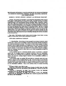
k and so the application of conventional (piecewise polynomial) boundary elements to this problem leads to full matrices of dimension at least N = O(k d−1 ) and a solution time of this order or worse as k → ∞. (Domain finite elements lead to sparse matrices but require even larger N .) Since this lack of robustness with respect to increasing values of k puts highfrequency problems beyond the reach of many standard algorithms, much recent research has been devoted to finding more robust methods. Of course, saying that k, which has dimension 1/length, is large is meaningless without reference to the size of the scatterer. The dimensionless quantity that can meaningfully be thought of as quantifying the oscillatory character of our problem is kL, where L is an appropriate characteristic length of the scattering surface Γ (e.g., the diameter of Γ). Thus a problem can be highly oscillatory even if k is not large provided that L is sufficiently large. But without loss of generality, throughout the review we consider k as the relevant large parameter, equivalently assuming that the unit of length is chosen so that the surface Γ has characteristic length O(1). The aim of this review is to describe a currently very active area of research which seeks algorithms for scattering problems which (ideally) have bounded error for fixed computational effort as k → ∞, and have computational complexity which is either independent of k, or grows only mildly as k increases. To achieve this aim, the methods we describe explicitly build into the numerical method a certain amount of asymptotic information about the oscillatory nature of the solution as k → ∞, and seek to approximate only the slowly varying components by (piecewise) polynomials. By now these methods have been supported by substantial theoretical justification, as we shall describe. It is well known that the scattering problem described above is in general a multiscale problem. Figure 1.1 illustrates the resulting total field u := uI + uS induced by a scatterer Ω− composed of the union of a disk and ˆ), a triangle, when the incident field uI is a plane wave uI (x) = exp(ikx · a with unit incident direction a ˆ. The scattered field uS is found as the solution of the classical ‘sound-soft’ scattering problem, that is, uS satisfies (1.1) in Ω+ , the Dirichlet condition uS = −uI (and so u = 0) on the scattering surface Γ (in this case the union of the circle and the boundary of the triangle) and, in addition, uS satisfies the usual Sommerfeld radiation condition (given by (2.9)) in the far field. While the incident field uI oscillates on the single scale k −1 , the total field u contains several other scales coming from the scattered field uS . These include scales of k −1/2 (respectively k −1/3 ) associated with widths of zones of transition from illuminated to shadow regions behind diffracting corners (respectively tangency points) These oscillatory and multiscale properties of scattered fields – known for many years in the asymptotics literature – are described in a form useful for numerical analysis in Section 3 of this review.

92


Figure 1.1. The total field when the incident field is a plane wave in the direction a ˆ = (cos θ, sin θ), with θ = −π/18, and the wavelength is λ = 0.2 (so k = 2π/λ = 10π ≈ 31.42). The scatterer has two components, a disk of unit diameter and a triangle.

To formulate BIEs for (1.1), we introduce the standard fundamental solution of the Helmholtz equation, given, in the two-dimensional (2D) and three-dimensional (3D) cases, by  i (1)     4 H0 (k|x − y|), d = 2, (1.2) Φk (x, y) :=  exp(ik|x − y|)   , d = 3,  4π|x − y| (1)

for x, y ∈ Rd , x = y, where Hν denotes the Hankel function of the first kind of order ν. Using Φk , we can build layer potentials that provide solutions to (1.1) in the exterior domain Ω+ , and automatically satisfy the radiation condition at infinity. These potentials conveniently also provide solutions to (1.1) in the interior domain Ω− . In general all the standard boundary value problems (BVPs) for the Helmholtz equation (1.1) can be formulated as integral equations on Γ using these layer potentials. For example, in the case of sound-soft scattering, the solution u is fully determined on Ω+ by its Neumann data ∂u/∂n on Γ; see Section 2 for details. Moreover the ‘far-field’ behaviour of u (often of interest in the solution of inverse scattering problems) can be determined by the action of a simple oscillatory linear operator applied to the Neumann data. The required Neumann data can be obtained, for example, by solving the combined potential

93


integral equation ∂Φk (x, y) ∂u 1 ∂u (x) + − iηΦk (x, y) (y) ds(y) = fk,η (x), 2 ∂n ∂n(x) ∂n Γ

x ∈ Γ,

(1.3) where, throughout the review, we adopt the convention that the normal derivative is taken outward from Ω− , and the source term is given by fk,η (x) :=

∂uI (x) − iηuI (x), ∂n

x ∈ Γ.

(1.4)

The problem (1.3) is well-posed for any fixed choice of the coupling parameter η ∈ R\{0} (see Theorem 2.46). We write (1.3) more compactly as 1 I + Dk − iηSk v = fk,η , where v := ∂u/∂n. (1.5) Ak,η v := 2 The operators Sk , Dk and Ak,η will be discussed in detail in Section 2. Turning to numerical methods, for an operator equation of the general form Av = f posed in L2 (Γ), the Galerkin method consists of choosing a finite-dimensional approximating space VN and then seeking an approximate solution vN ∈ VN such that (AvN , wN )L2 (Γ) = (f, wN )L2 (Γ) ,

for all wN ∈ VN .

(1.6)

For the discretization of the second-kind integral equation (1.5) there is a classical theory, which holds at least when Γ is sufficiently smooth and when the approximating space consists of piecewise polynomials. Suppose that we solve (1.5) using the Galerkin method (1.6) on a family of N dimensional spaces VN of piecewise polynomial functions of fixed degree on a quasi-uniform sequence of meshes on Γ with diameter h → 0 (so that N is proportional to h1−d ). Then it can be shown, using the methods in Atkinson (1997), for example, that there exist constants C > 0 and N0 > 0 such that the Galerkin solution vN satisfies the quasi-optimal error estimate v − vN ≤ C

inf

wN ∈VN

v − wN ,

(1.7)

for all N ≥ N0 , where here and throughout this review · represents · L2 (Γ) , unless otherwise specified. (This theory also extends to some collocation and, with the addition of quadrature, Nystr¨ om-like methods.) However, the classical theory does not tell us how C and N0 depend on k. These subtle questions are discussed in some detail in Section 6.1 of this review, but we can easily see that the error v − vN will be highly kdependent. This is because v is in general oscillatory, and the jth derivative of v will, roughly speaking, be O(k j ) times bigger than v itself. Thus, using standard estimates for piecewise polynomial approximation of degree p, the

94


error in best approximation appearing on the right-hand side of (1.7) will have an estimate of the form inf

wN ∈VN

v − wN ≤ C (hk)p+1 ,

(1.8)

for some constant C (which may itself grow with k). Thus h will need to decrease with O(k −1 ), and possibly faster, in order to keep the error bounded as k → ∞. Hence, standard (piecewise) polynomial BEMs applied directly to approximate the oscillatory solution v of (1.5) on a surface in Rd will have complexity at least O(h1−d ) = O(k d−1 ) as k → ∞. By contrast, the hybrid numerical-asymptotic methods which are the main subject of this review article exploit more detailed information about the oscillations in v (obtained via asymptotic analysis or exact integral representations) directly in the numerical method. Known highly oscillatory components of v are treated exactly in the algorithm, leaving only more slowly varying components to be approximated by piecewise polynomials. This yields a method which is much more ‘robust’ as k → ∞. One of the simplest hybrid numerical-asymptotic methods, and one which we shall discuss at length in Section 3, can be seen as an extension of the ‘physical optics’ (also called the ‘Kirchhoff’) approximation. This method assumes that the scattered wave uS oscillates on the same scale as the incoming plane wave, leading to the ansatz v(x) = kV (x, k) exp(ikx · a ˆ),

x ∈ Γ.

(1.9)

For some geometries (e.g., smooth convex scatterers), V (·, k) is much less oscillatory than v, and methods based on approximating V (·, k) using piecewise polynomials have been proposed by a number of authors. This procedure is equivalent to approximating v using a hybrid space VN with a basis consisting of products of the plane wave exp(ikx · a ˆ) and appropriate piecewise polynomial basis functions. Using such a hybrid space VN , it is possible to show that the best approximation error on the left-hand side of (1.8) increases much more slowly as k → ∞ than the estimate on the right-hand side of (1.8) (which holds for conventional piecewise polynomial spaces). Thus good approximation for large k on relatively coarse meshes (and with relatively few degrees of freedom) can potentially be achieved by hybrid methods. Unfortunately the benefits of these hybrid methods do not come without cost. When the mesh is fairly coarse and k is large, integration of the kernel of Sk or Dk over the support of a basis function requires computing an oscillatory integral. The additional oscillations arising via the basis functions further complicate these integrals, which have to be evaluated with a work count growing at worst modestly in k if the overall algorithm is to be


95

successful. Hence this field requires a substantial investment in research into numerical methods for oscillatory integrals; see Section 4 for details. To do a full numerical analysis of hybrid methods, not only do we require good estimates for the best approximation error (on the right-hand side of (1.7)), but also we need k-explicit estimates for the constants N0 and C in (1.7). This issue is discussed in Sections 5 and 6. Summarizing these points, one can think of the numerical analysis of hybrid methods as requiring research on three related questions. Q1 The design of k-dependent finite-dimensional approximation spaces VN , with the property that the best approximation error, that is, inf wN ∈VN v − wN , remains within a given tolerance as k → ∞, with N fixed or growing only slowly with k. Q2 The design of k-robust methods for computing the oscillatory integrals arising in implementation. Q3 The proof of sharp estimates for the dependence on k of the ‘stability constant’ C and the space dimension threshold N0 , ideally showing that these grow only slowly as k → ∞. This review describes research on these three fundamental issues and related topics, and we summarize its contents here. In Section 2 we describe fundamental solvability results on the relevant BVPs for (1.1) and the reformulation of these BVPs as BIEs, including new BIE formulations that have recently been proposed for high-frequency scattering problems. Given that many scatterers in applications involve corners and edges, we work on general Lipschitz domains. Background results for this section, some of which are not easily found in the literature, are given as an appendix. Section 3 describes the design of good hybrid spaces for a range of scattering problems and the proof of k-robustness of the best approximation error for these spaces (Q1). While this section is concerned mostly with 2D problems, hybrid spaces for a class of 3D screen problems are also discussed later in Section 7.6. In Section 4 the question of robust computation of oscillatory integrals which arise in hybrid methods is considered (Q2), and rigorous error estimates for these integration schemes, which have been the subject of recent research, are described. Section 5 describes the recently very active field which seeks k-explicit bounds on the conditioning of integral operators such as that in (1.5) (in particular, bounds on the operator, bounds on its inverse, coercivity properties, etc.). These results are required for estimating the constants N0 and C appearing in the formulation of Q3 above. This is done in Section 6, which in fact gives error estimates for standard as well as hybrid boundary element methods, valid as k → ∞. Finally, Section 7 presents a series of illustratory numerical examples, supporting the estimates of Section 6 and showing that, for a range of scattering

96


problems, arbitrary accuracy is achieved with a computational cost that grows only very mildly with respect to k. We finish this introduction with some historical remarks on the development of hybrid numerical-asymptotic methods, concluding with some remarks on other methods for the accurate solution of high-frequency scattering problems. Methods that combine numerical and asymptotic approaches in order to reduce computational cost have been applied within the electromagnetics community for many years. Two papers dating back to 1975 suggest reducing the computational cost at high frequencies by splitting the boundary into different regions, and using numerical methods in some regions and asymptotic approximations in others (Thiele and Newhouse 1975, Burnside, Yu and Marhefka 1975). The BIE method proposed in Burnside et al. (1975), for an electromagnetic problem equivalent to plane wave scattering by a sound-hard square, can sensibly be viewed as a prototype of the methods that we develop for scattering by convex polygons in Section 3.3 (and see Sections 7.2–7.4). The related method proposed in Thiele and Newhouse (1975) is a first instance of what has become a popular hybrid BIE-based methodology, whereby high-frequency physical optics approximations (see (3.4) below) are employed on part of the scattering surface, and standard BEM approximations on the remainder, with coupling between these subdomains: see Djordjević and Notaro˘s (2005), Zhang et al. (2010) and the references therein for recent developments. A hybrid numerical-asymptotic BIE method in exactly the sense of this article was proposed at almost the same time in the acoustics literature by Uncles. In a short proof-of-concept paper, Uncles (1976) proposed the use of essentially the ansatz (1.9), computing scattering by a sound-hard sphere using a piecewise constant approximation for the unknown V (·, k). This hybrid BIE idea (approximating the ratio of scattered to incident field rather than the scattered field itself) was used for the 2D problem of scattering by an impedance half-plane (which we treat with more sophisticated hybrid methods in Section 3.2), by Chandler-Wilde (1988), with numerical results demonstrating the efficiency of this approach at moderate frequencies. Essentially the same hybrid BIE method to that in Uncles (1976) was proposed independently in the electromagnetics literature in James (1990). Numerical results for the case of a circular scatterer (solving the integral equations (2.109) and (2.111) below) again demonstrated a significant reduction in the number of unknowns required compared to a conventional BEM. A more elaborate method, using hybrid spaces which are close to but less sophisticated than those described below in Sections 3.3.1–3.3.2, was proposed by Wang (1991), whose numerical results demonstrate some accuracy for a number of 2D geometries. The work of Aberegg and Peterson (1995) developed the methods of Uncles and Wang. To tackle 2D problems


97

of electromagnetic scattering by piecewise smooth convex obstacles, solving the Helmholtz equation (1.1), they used the same ansatz (1.9) but introduced a number of aspects that are key to the effective implementation of hybrid methods and which we will study in some detail in Section 3, namely higher-order basis functions, the treatment of corner singularities (via special basis functions in Aberegg and Peterson (1995)), and the use of mesh grading. They report, for many geometries, reasonably accurate results (≤ 3.5% relative error) with ten times fewer degrees of freedom compared to standard BEMs, and note that the method is robust in that, in cases where the ansatz (1.9) does not capture accurately the oscillation in the solution, the method should in any case be no less accurate for the same number of degrees of freedom than conventional BEMs. Since 1994 there has been significant numerical analysis interest in hybrid methods for scattering problems, with the majority of investigations focusing (either implicitly or explicitly) on the case of a smooth convex obstacle. This started with the contributions of Abboud et al. (1994, 1995), who considered (1.1) subject to an impedance boundary condition on Γ, and formulated this as a first-kind BIE, somewhat different to (1.3) (see (3.10) for details). The ansatz (1.9) was then applied, with the ‘slow variable’ V (·, k) being approximated using the h-version BEM. This analysis and numerical scheme was subsequently developed by Darrigrand (2002), who proposed fast multipole-based methods to evaluate the oscillatory integrals that arise. A more advanced approach than that taken by Abboud, Nédélec and Zhou (1995), taking special care to approximate V (·, k) accurately near the shadow boundary (see Section 3 for details), was proposed by Bruno, Geuzaine, Monro and Reitich (2004). They developed a high-frequency Nystr¨ om approach, substituting (1.9) directly into (1.5) to obtain a secondkind integral equation for the slow variable V (·, k) (see (3.11)), and then devising a frequency-robust, fast quadrature method for discretizing the corresponding integral operators. This was extended further, with strong emphasis on integration in 3D problems, by Bruno and Geuzaine (2007). At around the same time, Giladi and Keller (2004) – see also Giladi (2007) (following earlier work by Giladi and Keller (2001) on finite element methods) – solved the same equation considered by Bruno et al. (2004) using a collocation method, but also took into account the exponentially damped ‘creeping waves’ behind the shadow boundary. Subsequently Huybrechs and Vandewalle (2006) developed steepest descent-based methods for oscillatory integration and applied these in the implementation of a collocation-type scheme for the BIE (2.109), again using the ansatz (1.9) (Huybrechs and Vandewalle 2007b), with the advantage that their approach leads to a sparse linear system.

98


The same problem of scattering by a sound-soft smooth convex 2D obstacle was considered in Dom´ınguez, Graham and Smyshlyaev (2007), where the ansatz (1.9) was again used. By extending the asymptotic analysis of Melrose and Taylor (1985), Dom´ınguez et al. were able to derive rigorous estimates demonstrating that their Galerkin method achieved an error that depended only very mildly on k (see Section 3.1). For the problem of scattering by an impedance half-plane (see Section 3.2), Chandler-Wilde, Langdon and Ritter (2004), and then Langdon and Chandler-Wilde (2006), proposed and analysed a hybrid Galerkin BEM, proving rigorous error estimates independent of k, as k → ∞. These ideas were extended to scattering by sound-soft convex polygons (Chandler-Wilde and Langdon 2007, Hewett, Langdon and Melenk 2012), curvilinear polygons (Langdon, Mokgolele and Chandler-Wilde 2010), convex polygons with impedance boundary conditions (Chandler-Wilde, Langdon and Mokgolele 2012b), and non-convex polygons (Chandler-Wilde, Hewett, Langdon and Twigger 2012a), and are described in detail in Sections 3.3 and 3.4. A Galerkin method in the same spirit, utilizing a high-frequency ansatz similar to those described in Section 3, was applied to the 2D problem of scattering by a flat strip in Davis and Chew (2008), with numerical results suggesting only a very mild dependence of the error on the frequency. For the case of scattering by a smooth convex obstacle in 3D, Ganesh and Hawkins (2011) again used the ansatz (1.9), and the integral equation for V (·, k) was solved using a discrete Galerkin method with a global polynomial basis and a specially chosen global quadrature rule to handle the oscillatory integrals. The design of hybrid spaces for the case of multiple scattering (scattering by two or more disjoint convex scatterers) has been considered by Geuzaine, Bruno and Reitich (2005), and a detailed analysis of the phase structure of the solution has been given in Ecevit (2005), Ecevit and Reitich (2009) and Anand, Boubendir, Ecevit and Reitich (2009). Further discussion of many of the above approaches will be given in Sections 3 and 4. Due to space considerations, this review has not been able to discuss in detail three other techniques which also address the efficient solution of high-frequency scattering problems, and here we give only a few representative references. The first seeks fast implementations (often specifically tuned to the highfrequency case) of standard discretization methods and includes fast multipole and related fast iterative methods. Research in this direction is still very active and here we mention Rokhlin (1990), Amini and Maines (1998), Christiansen and Nédélec (2000), Farhat, Macedo and Lesoinne (2000), Bruno and Kunyansky (2001), Chandler-Wilde, Rahman and Ross (2002), Donepudi, Jin and Chew (2003), Harris and Chen (2003), Darve and Havé (2004), Livschits and Brandt (2006), Erlangga, Oosterlee and Vuik


99

(2006), Engquist and Ying (2007), Banjai and Hackbusch (2008), Bruno, Dom´ınguez and Sayas (2012), Ernst and Gander (2012) and Engquist and Ying (2012). The second is research on partition of unity and related methods in which a number of plane waves is introduced on each element in addition to standard piecewise polynomial boundary elements. These methods are accurate and rapidly convergent for general Helmholtz problems and do not require any prior knowledge of the asymptotics of the solution, but they do not enjoy the k-robustness of the hybrid methods for classes of scattering problems which we describe in this review; in particular, in each of these methods, the degrees of freedom need to increase in proportion to k d−1 to maintain accuracy as k → ∞, just as for conventional BEMs, albeit with a lower constant of proportionality. Examples of this approach include de La Bourdonnaye (1994), Perrey-Debain, Trevelyan and Bettess (2003a), Perrey-Debain, Trevelyan and Bettess (2003b), de La Bourdonnaye and Tolentino (2004), Perrey-Debain, Laghrouche, Bettess and Trevelyan (2004), Perrey-Debain, Trevelyan and Bettess (2005), and Honnor, Trevelyan and Huybrechs (2010). There also exists an extensive literature applying similar ideas within a finite element context; see, for example, Melenk and Babuˇska (1996), Babuˇska and Melenk (1997), Cessenat and Després (1998), Monk and Wang (1999), Giladi and Keller (2001), Laghrouche, Bettess and Astley (2002), Huttunen, Monk and Kaipio (2002), Cessenat and Després (2003), Laghrouche, Bettess, Perrey-Debain and Trevelyan (2005), Buffa and Monk (2008), Gittelson, Hiptmair and Perugia (2009), Luostari, Huttunen and Monk (2009), Hiptmair, Moiola and Perugia (2011a) and Esterhazy and Melenk (2012). The third is the solution of appropriate limiting problems, which are valid only if the frequency is sufficiently high (so-called ‘ray tracing’ methods). Considerable progress has been made on extending these to practical geometries and obtaining error estimates; see, for example, Engquist and Runborg (2003), Benamou (2003), Bleszynski, Bleszynski and Jaroszewicz (2004) and Motamed and Runborg (2009). Finally we mention that earlier reviews on the subject matter of this article include Bruno and Reitich (2007) and Chandler-Wilde and Graham (2009). We finish with a brief word on notations and assumed prior knowledge. Throughout we use function space notations that are explained in the Appendix (with cross-referencing from other sections). This use is mild in the more algorithmic Sections 3, 4, and 7, and more pronounced in Sections 2, 5, and 6, where we also need some functional analysis concepts and results which are briefly listed with references at the beginning of the Appendix. We are a little cavalier throughout as to whether we write γu (the trace of u) or u|Γ (the restriction of u to Γ) for the value of the total field on Γ,

100


and likewise whether we write ∂n u or ∂u/∂n for the normal derivative. The distinction in these definitions, and that they coincide for the scattering problems that we study, is explained in Section 2.1 (see Theorem 2.12) and Section 2.8.

2. BVPs and integral equation formulations In this section we formulate the relevant BVPs for the Helmholtz equation, giving details as appropriate of function spaces, radiation conditions, etc. We also formulate BIEs, and study properties of the layer potentials and integral operators which these give rise to. We make explicit the relationship between integral equations and BVPs, in particular the conditions under which BIE and BVP formulations are equivalent. There is much in this section regarding the theory of BIEs for acoustic problems which is not found in other reviews or monographs, in part because many of the results we describe are very recent. In particular, we develop new BIE formulations and new representations for boundary integral operators, which are essential components in the wavenumber-explicit error and stability analysis in Sections 5 and 6. However, those readers whose primary interest is in the design of hybrid algorithms and their implementation may well prefer to start with Sections 3 and 4, which can be read largely independently of this section. This article is concerned with scattering problems, so that our focus is naturally on exterior BVPs, that is, problems set in the unbounded exterior of a scatterer. But the theory of BIEs, particularly perhaps BIEs for acoustic problems, depends inextricably on an understanding of the well-posedness of both interior and exterior BVPs, so that necessarily we shall consider interior problems too. When it comes to the formulation of BVPs and BIEs, there is a degree of choice in the function space setting, in the sense in which the boundary conditions are to be understood, and indeed in the class of domains that one wishes to consider. Overwhelmingly the literature of the modern theory of BIE methods and their numerical solution, especially the solution of these problems on non-smooth domains, uses Sobolev space settings, for which a standard reference is McLean (2000). There is some variation in notations and definitions in respect of Sobolev spaces. We spell out our definitions precisely in the Appendix, mainly following McLean (2000), which has become a standard reference for the theory of BIEs on Lipschitz domains, but indicating explicitly wherever our notations and definitions vary from those of McLean, in which case we usually follow Sauter and Schwab (2011). For many of the scattering problems we consider, formulations in spaces of continuous functions, or Hölder-continuous functions, are also possible, particularly where the boundary is sufficiently smooth. A standard


101

reference for these is Colton and Kress (1983). We will indicate to what extent and under what conditions these formulations are equivalent in what follows. Some of the results that we wish to use and develop in this article are associated with a third setting for the BVPs, that associated with the harmonic analysis of Calder´ on–Zygmund operators on the boundaries of Lipschitz domains. There one studies BVPs with data in Lp spaces, understands boundary conditions to hold in a sense of almost everywhere non-tangential convergence, and supplements this with a requirement on the behaviour of maximal functions. Much of the above material, in particular the deep results using harmonic analysis methods, is not available in an accessible form in the BIE literature, and their implications for BIE methods are not fully understood. At the same time a number of the recent results which we will describe, and which are key to a rigorous error analysis of the new boundary element methods that we will propose, make essential use of these methods of analysis. For this reason the Appendix includes a brief account of these results, which use function spaces specified in terms of maximal functions, and of the relationship of these function spaces to usual Sobolev spaces. 2.1. Acoustic boundary value problems All the BVPs that we consider are for the Helmholtz equation (1.1) with wavenumber k, which arises in acoustics from the wave equation, satisfied by the perturbation in pressure on an assumption of harmonic (e−iωt ) time dependence. We will impose most often the sound-soft or Dirichlet boundary condition, namely that u is specified on the boundary Γ, which has been the focus of most of the theory and computation for hybrid numericalasymptotic methods to date. We will also show numerical results and analysis for problems where an impedance boundary condition (much more widely used in acoustic modelling) is imposed. This is ∂u − ikβu = h (2.1) ∂n on Γ, where n is the normal directed outwards from the domain of propagation, and β is the normalized admittance of the surface. In general β is a function of position (and generally also a function of frequency ω), given by β = ρc/ζ, where ζ is the surface impedance, and ρ the density of the fluid in which the acoustic wave propagates; the product ρc is termed the impedance of the medium of propagation. The h in (2.1) is given; usually h = 0 in scattering problems whenever u denotes the total field. Physical considerations, namely the requirement that the boundary does not emit energy, imply that Re β ≥ 0.

(2.2)

102


In the special case β = 0, the impedance boundary condition reduces to the Neumann or sound-hard boundary condition. One of many examples where (2.1) is a widely used boundary condition is in outdoor noise propagation, an application we will return to in Section 3.2, where (2.1) with β = 0 is an appropriate boundary condition on a hard road surface, while (2.1), with Re β > 0 and frequency dependent, is a widely used model of a range of sound-absorbing outdoor surfaces; e.g., Taraldsen and Jonasson (2011). This review contains some new BIE methods which give rise to the study of a generalization of the above boundary condition. Let Z be a bounded vector field defined (at least) on the boundary Γ. The generalization we make replaces the normal derivative in the boundary condition by an oblique derivative, so that the boundary condition is Z · ∇u − ikβu = h

(2.3)

on Γ. We will formulate all of our problems in the Sobolev space setting, and selected problems also in alternative function space settings. In the interior problems below, D is a bounded Lipschitz domain (see Definition A.2 and the paragraph that follows that definition) with boundary Γ, and γ is the trace operator (see Section A.3). We state first the interior Dirichlet problem: Given h ∈ H 1/2 (Γ), find u ∈ C 2 (D) ∩ H 1 (D) such that (1.1) holds in D and γu = h on Γ.

(2.4)

The solvability of this standard interior problem is well understood, e.g., McLean (2000, p. 286). Theorem 2.1. There exists a sequence 0 < k1 < k2 < · · · of positive wavenumbers, with km → ∞ as m → ∞, such that the interior Dirichlet problem with h = 0 has a non-trivial solution. For all other values of k > 0 the interior Dirichlet problem has exactly one solution. The other interior BVPs that are relevant to us are the interior impedance problem and what we will call the interior oblique impedance problem, by which we will mean the Helmholtz equation subject to the boundary condition (2.3). Note that, in these Sobolev space formulations, we understand the normal derivative of u in (2.1) as ∂n u ∈ H −1/2 (Γ), where ∂n is the normal derivative operator defined in equation (A.28). (Of course – see (A.18) – ∂n u coincides with classical definition of the normal derivative ∂u/∂n when u is sufficiently regular.) We understand the oblique derivative Z · ∇u as meaning Z · ∇u = Zn ∂n u + Z · ∇Γ γu, where Zn := Z · n is the normal component of Z and ∇Γ is the surface

103


gradient operator (see (A.14)). Thus the interior impedance problem is Given h ∈ H −1/2 (Γ), and β ∈ L∞ (Γ), find u ∈ C 2 (D) ∩ H 1 (D) such that (1.1) holds in D and ∂n u − ikβγu = h on Γ;

(2.5)

and the interior oblique impedance problem is Given h ∈ L2 (Γ), Z ∈ (L∞ (Γ))d , and β ∈ L∞ (Γ), find u ∈ C 2 (D) ∩ H 1 (D), with γu ∈ H 1 (Γ), such that (1.1) holds in D and Zn ∂n u + Z · ∇Γ γu − ikβ γu = h on Γ.

(2.6)

Note that the requirement, in (2.5), that ∂n u = h + ikβγu holds, means, in view of the definition of the normal derivative operator ∂n in (A.28) and (A.29), nothing more or less than the requirement that h γv ds + ik β γu γv ds = ∇u · ∇¯ v + v¯ ∆u dx, v ∈ H 1 (D), (2.7) Γ

Γ

D

2 −1/2 (Γ) but h ∈ L2 (Γ), in the case that

h ∈ L (Γ). In the case that h ∈ H the integral Γ h γv ds in (2.7) is understood as the limit h γv ds = lim hj γv ds, Γ

j→∞ Γ

where (hj ) ⊂ L2 (Γ) is any sequence which is convergent to h in the H −1/2 (Γ) norm. The boundary condition in (2.6) has an analogous interpretation to that of (2.7). The part of the solvability theory for the interior impedance BVP that we need (Colton and Kress 1983, McLean 2000) is encapsulated in the following theorem. In the statement of this theorem we make the first reference to the following assumption. Assumption 2.2. Either: (a) Re β ≥ 0 and Re β > 0 on some relatively open subset of Γ; or: (b) Re β ≤ 0 and Re β < 0 on some relatively open subset of Γ. Theorem 2.3. (i) Suppose that Assumption 2.2 holds. Then the interior impedance problem has exactly one solution. (ii) Suppose that β = 0 (the Neumann boundary case). Then there exists a sequence 0 = k1 < k2 < · · · of positive wavenumbers, with km → ∞ as m → ∞, such that the interior impedance problem with h = 0 has a non-trivial solution. For all other values of k > 0 the interior impedance problem with β = 0 has exactly one solution.

104


The existence statement in (i) can be obtained by a variety of arguments, not least by BIE methods as a corollary of Theorem 2.30 below. The uniqueness statement in (i) is a consequence of (2.7). In more detail, if u1 and u2 are solutions of (2.5) then, defining u := u1 − u2 , it follows from (2.7) applied with v = u, since ∆u = −k 2 u, that 2 ik β |γu| ds = |∇u|2 − k 2 |u|2 dx. (2.8) Γ

D

Taking imaginary parts, we see that Γ Re β|γu|2 ds = 0, so that in case (i) we deduce that γu vanishes on some relatively open subset of Γ. Since ∂n u = ikβγu, it follows that ∂n u vanishes on the same open subset of Γ. By the following version of Holmgren’s uniqueness theorem it follows that u is identically zero and so u1 = u2 . Theorem 2.4. Suppose that D is a bounded Lipschitz open set and that u ∈ C 2 (D) ∩ H 1 (D) satisfies the Helmholtz equation (1.1) in D and γu = ∂n u = 0 on Γ0 , some non-empty, relatively open subset of Γ = ∂D. Then u = 0 (in D). Proof. Let G = (Rd \Γ)∪Γ0 , so that G is the open set which is the union of Γ0 and the interior and exterior of Γ. Extend the definition of u from D to G by setting u(x) = 0 for x ∈ G \ D. Then it follows from Theorem 2.20 below that u in G\Γ0 is the difference of two layer potentials, each with density that vanishes on Γ0 . Hence, by Theorem 2.14, u ∈ C 2 (G) and (1.1) holds in G. But (see, e.g., Colton and Kress 1983) solutions of the Helmholtz equation in a domain are real analytic in that domain and, if they vanish in some open subset, vanish identically. Thus u = 0 in the component of G that includes D ∪ Γ0 , and in particular u = 0 in D. Of course, the focus of this article is on solving exterior problems in unbounded domains, for which radiation conditions need to be imposed to ensure uniqueness of solution, expressing mathematically the physical idea that any acoustic field is radiating away from the physical boundary. In the case when the Helmholtz equation (1.1) holds outside some bounded set, the standard radiation condition to impose is the Sommerfeld radiation condition, that ∂u (x) − iku(x) = o(r−(d−1)/2 ), (2.9) ∂r as r := |x| → ∞, uniformly in x ˆ := x/r. The following lemma is an important consequence of this radiation condition; for a proof see, e.g., Colton and Kress (1983). In this lemma, and the remainder of the article, we use the notations BR := {x ∈ Rd : |x| < R}, ΓR := ∂BR = {x : |x| = R}, and Sd−1 := {x ∈ Rd : |x| = 1}.

105


Lemma 2.5. If, for some R > 0, u satisfies (1.1) in Rd \ BR and the Sommerfeld radiation condition (2.9), then there exists a function F ∈ C ∞ (Sd−1 ) (the far-field pattern) such that u(x) =

eikr

r(d−1)/2

F (ˆ x) + O(r−1 )

(2.10)

as r → ∞, uniformly in x ˆ := x/r. A consequence of Lemma 2.5 is the following lemma, derived by applying Green’s first identity (A.29) to u in the domain BR ∩ Ω+ and then letting R → ∞. In this lemma and for the next paragraphs up to and including Theorem 2.10, we suppose that Ω− is a bounded Lipschitz open set such that Ω+ := Rd \ Ω− is a Lipschitz domain with boundary Γ = ∂Ω+ . In this configuration, as noted in Sections 1 and A.5, the normal vector n will 1 (Ω ) is as defined always be taken to point out from Ω− into Ω+ , and Hloc + in (A.30). 1 (Ω ) and u satisfies the Helmholtz Lemma 2.6. If u ∈ C 2 (Ω+ ) ∩ Hloc + equation (1.1) in Ω+ and the Sommerfeld radiation condition (2.9), then 2 2 2 |∇u| − k |u| dx = I − γ u ¯ ∂n u ds (2.11) Ω+

where

I := lim

R→∞ ΓR

u ¯

Γ

∂u ds = ik lim R→∞ ∂r

|u|2 ds = ik ΓR

Sd−1

|F (ˆ x)|2 dˆ x,

is understood as the improper integral and the integralover Ω+ in (2.11) limR→∞ BR ∩Ω+ |∇u|2 − k 2 |u|2 dx. We will study, in the unbounded domain Ω+ , the exterior Dirichlet problem: 1 (Ω ) such that (1.1) holds Given h ∈ H 1/2 (Γ), find u ∈ C 2 (Ω+ ) ∩ Hloc + in Ω+ , γu = h on Γ, and u satisfies the radiation condition (2.9). (2.12)

We will also study the exterior impedance problem: Given h ∈ H −1/2 (Γ) and β ∈ L∞ (Γ), find u ∈ C 2 (Ω+ )∩ 1 (Ω ) such that (1.1) holds in Ω , ∂ u + ikβu = h on Γ, Hloc + + n and u satisfies the radiation condition (2.9).

(2.13)

(The sign change in this impedance boundary condition compared to (2.1) is because the normal n here points into the domain of propagation.) In contrast to the interior Dirichlet and Neumann problems, both problems (2.12) and (2.13) have at most one solution for all k > 0. This is a consequence of Lemma 2.8 below, which in turn follows from the following key lemma due to Rellich (for a proof see Colton and Kress 1983).

106


Lemma 2.7. (Rellich) If u ∈ C 2 (Ω

+ ) satisfies (1.1) in Ω+ and the radiation condition (2.9), and limR→∞ ΓR |u|2 ds = 0, then u is identically zero. Rellich’s lemma implies the following result (Colton and Kress 1983). 1 (Ω ) satisfies (1.1) in Ω , the radiation Lemma 2.8. If u ∈ C 2 (Ω+ ) ∩ Hloc + + condition (2.9), and γu ¯∂n u ds ≤ 0, Im Γ

then u = 0 (in Ω+ ). Proof.

The conditions of the lemma imply, by Lemma 2.6, that 2 |F (ˆ x)| dˆ x = Im γu ¯∂n u ds ≤ 0, k Sd−1

(2.14)

Γ

so that F = 0 in L2 (Sd−1 ). It follows from Lemma 2.6 that |u|2 ds = 0 lim R→∞ ΓR

and hence, by Rellich’s lemma, that u = 0. An immediate consequence of Lemma 2.8 is the following uniqueness result for the exterior Dirichlet and impedance problems. Corollary 2.9. The exterior Dirichlet BVP (2.12) and the exterior impedance BVP (2.13), with Re β ≥ 0, each have at most one solution. Corollary 2.9 is the uniqueness part of the following theorem. Theorem 2.10. The exterior Dirichlet BVP and the exterior impedance BVP, with Re β ≥ 0, each have exactly one solution. Proof. Existence follows from Corollary 2.28 below, which uses results about invertibility of boundary integral operators. Our prime interest in the above exterior Dirichlet and impedance problems is that they arise in the context of acoustic scattering. By acoustic scattering we mean the problem of computing the scattered acoustic field uS produced when an incident field uI interacts with an obstacle or obstacles (the scatterer ) occupying some closed set Ω, such that Ω+ := Rd \ Ω is an unbounded domain. By an incident field we mean the following. Definition 2.11. We call uI ∈ L1loc (Rd ) an incident field if, for some open neighbourhood G of Ω, uI |G ∈ C ∞ (G) and satisfies the Helmholtz equation (1.1) in G. We will refer throughout to the sum u := uI + uS as the total acoustic field (total field for short).

107


We deal exclusively with the case when Ω is bounded, except in Section 3.2. Further, except in Section 7.6, we deal exclusively with the case where Ω = Ω− , with Ω− , the interior of Ω, a Lipschitz open set, in which case Γ, the surface of the scatterer, is the common boundary of Ω+ and Ω− . We will focus particularly on the case when the incident field is a plane a| = 1, wave, that is, for some a ˆ ∈ Rd with |ˆ ˆ), uI (x) = exp(ikx · a

x ∈ Rd .

However, many of our results apply to general incident fields, for example the field generated by a point source, that is, for some z ∈ Rd \ Ω, uI (x) = Φk (x, z),

x ∈ Rd \ {z},

where Φk is the fundamental solution of the Helmholtz equation defined in (1.2). In this article we will focus on the cases of the sound-soft scatterer (where u = 0 on Γ), the impedance scatterer, where (2.13) with h = 0 holds on Γ, and the sound-hard scatterer, the special case of the impedance scatterer in which ∂u/∂n = 0 on Γ. Considering first the sound-soft scattering problem, one natural formulation, where our requirement on uS is continuity rather than membership of a particular Sobolev space, is the following: Find uS ∈ C 2 (Ω+ ) ∩ C(Ω+ ) such that (1.1) holds in Ω+ , u = 0

(2.15)

(so uS = −uI ) on Γ, and uS satisfies the radiation condition (2.9). In the case that Ω+ is a Lipschitz domain, a second natural formulation is to require that the scattered field uS satisfy the exterior Dirichlet problem (2.12), with boundary data −uI |Γ . In other words uS satisfies: 1 (Ω ) such that (1.1) holds in Ω , γu = 0 (2.16) Find uS ∈ C 2 (Ω+ ) ∩ Hloc + +

(so γuS = −uI |Γ ) on Γ, and uS satisfies the radiation condition (2.9). It is shown in Colton and Kress (1998, Theorem 3.7) that problem (2.15) has at most one solution, and the argument in the proof of that theorem shows that if uS satisfies (2.15) and Ω+ is Lipschitz, then uS satisfies (2.16). Further, in the case that Ω+ is Lipschitz, it is a corollary of Theorem 2.10 that (2.16) has exactly one solution which also satisfies (2.15); to see this it is a matter of showing that if uS satisfies (2.16) then uS ∈ C(Ω+ ). This does not follow from the Sobolev embedding theorem (Theorem A.1), but is a consequence of elliptic regularity results up to the boundary; e.g., Kenig (1994). Thus the following result holds. Theorem 2.12. The Dirichlet scattering problem (2.15) has at most one solution. In the case that Ω+ is a Lipschitz domain, (2.15) and (2.16) share the same unique solution, which satisfies ∂n u ∈ L2 (Γ).

108


Proof. In view of the discussion above it remains only to show that ∂n u ∈ L2 (Γ). But, by Definition 2.11, for some neighbourhood G of Γ, uI |G ∈ C ∞ (G) so that uI |Γ ∈ C ∞ (Γ) ⊂ H 1 (Γ) (see Section A.3). Thus γuS ∈ H 1 (Γ), and the fact that ∂n u ∈ L2 (Γ) follows from Theorem A.5. We remark that, while it is common (following the lead of Colton and Kress 1983, for instance) to make use of the formulation (2.15) in the case when Ω+ is sufficiently smooth, precisely when Ω+ is C 1,µ for some µ ∈ (0, 1], overwhelmingly the recent numerical analysis literature for the case of Lipschitz Ω+ uses the formulation (2.16). Theorem 2.12 makes clear that the formulation (2.15) is a valid alternative even in the Lipschitz case. Consider next the impedance scattering problem formulated as follows. Restricting attention to the case when Ω+ is Lipschitz, we require that uS satisfies the exterior impedance problem (2.13) with I ∂u I + ikβu ∈ L2 (Γ). h := − (2.17) ∂n Γ In other words, with h given by (2.17), uS satisfies: 1 (Ω ) such that (1.1) holds in Find uS ∈ C 2 (Ω+ ) ∩ Hloc +

Ω+ , ∂n u + ikβγu = 0 (so ∂n uS + ikβγuS = h) on Γ, and

uS

(2.18)

satisfies the radiation condition (2.9).

Analogously to Theorem 2.12, an immediate corollary of Theorem 2.10 and Theorem A.5, is the following result. Corollary 2.13. The impedance scattering problem (2.18) has exactly one solution, which satisfies ∂n u ∈ L2 (Γ) and γu ∈ H 1 (Γ). 2.2. Layer potentials In Section 2.5 we will formulate the BVPs in the previous subsection as BIEs. Here we introduce the required layer potentials and recall some of their properties. Suppose that Ω+ is an unbounded Lipschitz open set with boundary Γ, in which case Ω− := Rd \ Ω+ is a bounded Lipschitz open set. For φ ∈ L1 (Γ) and k > 0 let Φk (x, y)φ(y) ds(y), x ∈ Rd \ Γ, (2.19) Sk φ(x) := Γ

and

Dk φ(x) :=

Γ

∂Φk (x, y) φ(y) ds(y), ∂n(y)

x ∈ Rd \ Γ,

(2.20)


109

where the normal n is directed into Ω+ . Note that, in particular, these definitions apply for φ ∈ H s (Γ) with 0 ≤ s ≤ 1, since of course H s (Γ) ⊂ L2 (Γ) ⊂ L1 (Γ). Further, they extend in a natural way, via the duality pairing ·, ·Γ defined by (A.24), to the case that φ ∈ H s (Γ) for −1 ≤ s < 0. In this case, for example, noting that Φk (x, ·) ∈ C ∞ (Γ) ⊂ H −s (Γ), Sk φ(x) is understood as Sk φ(x) = Φk (x, ·), φΓ , and Dk φ(x) is understood similarly. Equivalently, Sk φ(x) and Dk φ(x) can be understood as the limits Sk φ(x) = lim Sk φj (x), j→∞

Dk φ(x) = lim Dk φj (x), j→∞

(2.21)

where (φj ) ⊂ L2 (Γ) is any sequence converging in H s (Γ) to φ ∈ H s (Γ). We will use the above definitions also for k = 0 with Φ0 given by (1.2) in the 3D case (d = 3). The definition (1.2) does not make sense when d = 2 and here we define Φ0 by a 1 log , (2.22) Φ0 (x, y) := 2π |x − y| for some constant a > 0 (the usual choice a = 1). In both 2D and 3D, Φ0 is the standard fundamental solution for the Laplace equation. Boundary integral equation methods for solving the BVPs of Section 2.1 are based on solutions in terms of layer potentials. This is effective because of the following simple result whose proof we sketch. Theorem 2.14. For k ≥ 0 and φ ∈ H −1 (Γ), Sk φ, Dk φ ∈ C 2 (Rd \ Γ) and satisfy (1.1) in Rd \ Γ. For k > 0, Sk φ and Dk φ satisfy the Sommerfeld radiation condition (2.9). Proof. For a proof in the case that φ ∈ C(Γ), see Colton and Kress (1983). For Sk φ the result follows for φ ∈ H −1 (Γ) since C(Γ) is dense in H −1 (Γ), so that there exists a sequence (φj ) ⊂ C(Γ) with φ − φj H −1 (Γ) → 0 as j → ∞, which implies that Sk φj (x) → Sk φ(x) uniformly on compact subsets of Rd \ Γ, from which it follows that Sk φ satisfies (1.1). In the case k > 0 also, for all sufficiently large R, max |x| |Sk φj (x) − Sk φ(x)| → 0, as j → ∞, |x|≥R

from which it follows that Sk φ satisfies the Sommerfeld radiation condition. The same arguments work for Dk φ when φ ∈ H −1 (Γ). The above theorem, coupled with Lemma 2.5, implies that, for k > 0, Sk φ and Dk φ both have the representation (2.10) at infinity. In fact (see Colton and Kress 1998, or McLean 2000, p. 294), the far-field patterns of

110


Sk φ and Dk φ are, respectively, x) = c d k FS (ˆ

exp(−ikˆ x · y)φ(y) ds(y)

(d−3)/2

and

(2.23)

Γ

x) = −i cd k (d−1)/2 FD (ˆ

x ˆ · n(y) exp(−ikˆ x · y)φ(y) ds(y),

(2.24)

Γ

where cd =

e−i(d−3)π/4 . 2(2π)(d−1)/2

To derive BIEs for scattering problems, we need to supplement the above result with mapping properties of Sk and Dk . In the following theorem, χ ∈ C0∞ (Rd ) is any smooth compactly supported function such that χ(x) = 1 in a neighbourhood of Ω− ∪ Γ and, for example, χSk denotes the composition of the operator Sk followed by multiplication by χ. A consequence 1 (Rd ) and that D φ ∈ H 1 (Ω ). (From of Theorem 2.15 is that Sk φ ∈ Hloc ± k loc (2.23) and (2.24) it follows that Sk φ and Dk φ decay too slowly at infinity for either to be in H 1 (Ω+ ).) Theorem 2.15. bounded:

For − 12 ≤ s ≤

1 2

and k ≥ 0, the following mappings are

(i) χSk : H s−1/2 (Γ) → H s+1 (Rd ); (ii) χDk : H s+1/2 (Γ) → H s+1 (Ω± ). A proof of the above theorem for the restricted range |s| < 1/2, derived from the key paper by Costabel (1988), is given in McLean (2000). It depends on characterizations of the single- and double-layer potential operators in terms of the adjoints of the trace and normal derivative operators, respectively, and, in particular, depends on (A.17), which holds only for 1/2 < s < 3/2 and not for s = 1/2 (even for smooth boundaries Γ). Thus the proof does not extend to s = ±1/2. This is of significance for us since, for the most part, it will be precisely the limiting cases s = ±1/2 that are of interest. To establish the mapping properties of Theorem 2.15 for s = ±1/2 (which, as McLean notes, imply the same mapping properties for |s| < 1/2 by interpolation), we can use the equivalences of Corollary A.8. These, together with the standard interpolation results, imply that Theorem 2.15 is equivalent to Theorem 2.16 below. In this theorem, the so-called non-tangential maximal functions, u∗ and (∇u)∗ , are defined as in (A.36) and (A.37), except that now Θ(x) := Θ+ (x) ∪ Θ− (x), where {Θ± (x) : x ∈ Γ} denotes any uniform and sufficient family of non-tangential approach sets in Ω± , so that Θ± (x) ⊂ Ω± , Θ± (x) ∩ Γ = {x}, and (A.32) holds with the same constant C > 1 for every x ∈ Γ.

111


Theorem 2.16. For φ, ψ ∈ H −1 (Γ) let u = Sk φ and v = Dk ψ. Then, for some constant C > 0 independent of φ and ψ: (i) if φ ∈ L2 (Γ) then (∇u)∗ ∈ L2 (Γ) and (∇u)∗ L2 (Γ) ≤ CφL2 (Γ) ; (ii) if ψ ∈ L2 (Γ) then v ∗ ∈ L2 (Γ) and v ∗ L2 (Γ) ≤ CψL2 (Γ) ; (iii) if φ ∈ H −1 (Γ) then u∗ ∈ L2 (Γ) and u∗ L2 (Γ) ≤ CφH −1 (Γ) ; (iv) if ψ ∈ H 1 (Γ) then (∇v)∗ ∈ L2 (Γ) and (∇v)∗ L2 (Γ) ≤ CψH 1 (Γ) . The proof of this theorem requires deep results from the harmonic analysis literature, specifically that part concerned with the study of Calderón– Zygmund operators, in particular Cauchy integral and layer-potential operators on Lipschitz curves and surfaces. For a proof of (i) and (ii) we refer the reader to the account in Meyer and Coifman (2000) for the case k = 0 and Torres and Welland (1993) and Liu (1995) for the extension to k > 0. It is convenient to leave remarks on the proof of (iii) and (iv) (which are corollaries of (i) and (ii)) until we introduce relevant boundary integral operators in the next subsection. Note that by far the main part of the work is to establish results for k = 0. Extensions from k = 0 to k > 0 by perturbation arguments are relatively straightforward because Wk := Φk −Φ0 is much smoother than Φ0 . Precisely, it follows easily from (1.2) and the power series expansions for Hankel functions that Wk (x, y) = wk (x − y) where wk ∈ C ∞ (Rd \ {0}) and, for some constant ck > 0, ck log |x|−1 , d = 2, α |wk (x)| + |∇wk (x)| ≤ ck , |∂ wk (x)| ≤ (2.25) d = 3, ck |x|−1 , for |x| ≤ 1/2. Here α is any multi-index with |α| = 2 so that ∂ α wk is any second-order partial derivative (we use here the notation (A.1)). The monograph of Colton and Kress (1983) is a classic example of arguing by perturbation from k = 0 to obtain results for k > 0; see also Torres and Welland (1993), Liu (1995) and Mitrea (1996). As in Section A.5, we denote the exterior and interior trace operators by γ+ and γ− , and the exterior and interior normal derivative operators by ∂n+ and ∂n− , respectively, with the normal directed out of Ω− into the exterior domain Ω+ . Applying Theorem 2.15 with s = 0 and Theorem 2.14, we see that, for φ ∈ H −1/2 (Γ) and ψ ∈ H 1/2 (Γ), both χSk φ and χDk ψ are in H 1 (Ω± ), in fact in H 1 (Ω± ; ∆). (This notation is defined below equation (A.26).) It follows from (A.17) that the traces γ± Sk φ and γ± Dk ψ are welldefined as elements of H 1/2 (Γ), and that (see (A.28)) the normal derivatives ∂n± Sk φ and ∂n± Dk ψ are well-defined as elements of H −1/2 (Γ). Moreover (McLean 2000) the following jump relations hold: γ+ Sk φ = γ− Sk φ,

∂n+ Dk ψ = ∂n− Dk ψ.

(2.26)

112


A natural question to ask is whether the traces and normal derivatives of the single- and double-layer potentials, u = Sk φ and v = Dk ψ, have anything to do with the limiting values of u(x), v(x), ∇u(x) and ∇v(x) as x approaches Γ from inside Ω± . Reassuringly, this is the case, at least if the densities φ and ψ are smooth enough. As before Theorem 2.16, for x ∈ Γ let Θ± (x) denote any non-tangential approach set to x from Ω± , so that Θ± (x) ⊂ Ω± , Θ± (x) ∩ Γ = {x}, and (A.32) holds. Then, if φ ∈ H s−1/2 (Γ) and ψ ∈ H s+1/2 (Γ), for some s ∈ (−1/2, 1/2], it follows from Lemma A.9 that, for almost every x ∈ Γ, γ± u(x) =

lim

y→x, y∈Θ± (x)

u(y)

and

γ± v(x) =

lim

y→x, y∈Θ± (x)

v(y).

(2.27)

Further, these non-tangential limits are well-defined, by Theorem 2.16 and Corollary A.8, even for φ ∈ H −1 (Γ) and ψ ∈ L2 (Γ), providing an extension of the notion of the traces of u and v to the cases of densities φ ∈ H −1 (Γ) and ψ ∈ L2 (Γ). Similarly, if φ ∈ L2 (Γ) and ψ ∈ H 1 (Γ) then, by Theorem 2.16 and Lemma A.10, ∂n± u, ∂n± v ∈ L2 (Γ) and, for almost all x ∈ Γ, ∂n± u(x) =

∂u± (x) := lim n(x) · ∇u(y) ∂n y→x, y∈Θ± (x)

(2.28)

∂n± v(x) =

∂v± (x) := lim n(x) · ∇v(y). ∂n y→x, y∈Θ± (x)

(2.29)

and

Further, for almost all x ∈ Γ, by Theorem 2.16 and Lemma A.10, ∇Γ γu ∈ L2 (Γ) and lim

∇u(y) = ∇Γ γ± u(x) + n(x)∂n± u(x)

(2.30)

lim

∇v(y) = ∇Γ γ± v(x) + n(x)∂n± v(x).

(2.31)

y→x,y∈Θ± (x)

and y→x,y∈Θ± (x)

2.3. Boundary integral operators For k ≥ 0 we define the acoustic single- and double-layer operators, Sk and Dk , respectively, by Φk (x, y)φ(y) ds(y), Sk φ(x) := Γ (2.32) ∂Φk (x, y) φ(y) ds(y), Dk φ(x) := ∂n(y) Γ for x ∈ Γ, where Φk is given by (1.2) in 3D and in 2D by (1.2) for k > 0 and by (2.22) for k = 0.


113

When Γ and φ are both sufficiently smooth, it is well known that the above integrals are well-defined (the integrands are in L1 (Γ)) for all x ∈ Γ. In particular (Colton and Kress 1983), this is the case if Γ is C 2 and φ ∈ C(Γ), with both Sk φ, Dk φ ∈ C(Γ). In the 2D case, with φ ∈ L2 (Γ) and Γ Lipschitz, it still holds (by Cauchy–Schwarz, since Φk (x, ·) ∈ L2 (Γ) when d = 2), that Sk φ(x) is well-defined for all x ∈ Γ and Sk φ ∈ C(Γ). For Lipschitz Γ, the situation is more delicate for the double-layer potential, but for φ ∈ L2 (Γ), irrespective of the dimension d, Sk φ and Dk φ are well-defined by (2.32) for almost all x ∈ Γ, with Dk φ understood as the Cauchy principal value integral ∂Φk (x, y) φ(y) ds(y), x ∈ Γ, (2.33) Dk φ(x) := lim →0 Γ\B (x) ∂n(y) where B (x) is the open ball of radius centred at x and Sk φ, Dk φ ∈ L2 (Γ). This result for the double-layer potential is not straightforward and was established first for the case k = 0; see, e.g., Meyer and Coifman (2000) and the discussion in the following paragraphs. The extension to k > 0 is more straightforward; see Torres and Welland (1993). As is well known, and will be recalled below, Sk φ and Dk φ appear when we take boundary values of the single- and double-layer potentials Sk φ and Dk φ. When we apply the normal derivative operator ∂n , two additional boundary integral operators, Dk and Hk , arise, which we will term the (acoustic) adjoint double-layer operator and the (acoustic) hypersingular operator, respectively. For φ ∈ L2 (Γ) and ψ ∈ H 1 (Γ) these operators are given explicitly by ∂Φk (x, y) φ(y) ds(y), (2.34) Dk φ(x) := ∂n(x) Γ ∂ ∂Φk (x, y) ψ(y) ds(y), (2.35) Hk ψ(x) := ∂n(x) Γ ∂n(y) for almost all x ∈ Γ, where the integral defining Dk φ is understood as a Cauchy principal value integral (as in (2.33)) while Hk ψ ∈ L2 (Γ) is defined in the sense of (2.29), that is, Hk ψ(x) :=

lim

y→x, y∈Θ± (x)

n(x) · ∇Dk ψ(y).

(2.36)

Note that for ψ ∈ H 1/2 (Γ), ∂n+ Dk ψ = ∂n− Dk ψ (see (2.26)). It follows from (2.29) that the limits in (2.36) as y → x from Θ+ (x) and from Θ− (x) coincide. It is a consequence of Young’s inequality for convolutions that Sk is a bounded operator on L2 (Γ). A much deeper result is that both Dk and Dk are bounded operators on L2 (Γ); for a clear discussion of the proofs of these results for k = 0 see Meyer and Coifman (2000), and see Torres

114


and Welland (1993) for the relatively straightforward extensions to k > 0. This boundedness was established only in 1982 as a corollary of the proof of Coifman, McIntosh and Meyer (1982) that the Cauchy integral operator is bounded on L2 (Γ) when Γ is the graph of a Lipschitz-continuous function. It was shown soon afterwards, by Verchota (1984), that, in the case k = 0, Dk is also a bounded operator on H 1 (Γ) and Sk a bounded operator from L2 (Γ) to H 1 (Γ); again, for extensions to k > 0 see Torres and Welland (1993). The results in Verchota (1984) were achieved through the use of Rellich-type identities, which we will make new use of in Section 5.7 (see the discussion in Section 5.3). Important identities, which follow by Fubini’s theorem for Sk , and by the arguments of Meyer and Coifman (2000) plus Fubini’s theorem (to move from k = 0 to k > 0) for Dk and Dk , are that, for φ, ψ ∈ L2 (Γ), φ Sk ψ ds = ψ Sk φ ds, φ Dk ψ ds = ψ Dk φ ds. (2.37) Γ

Γ

Γ

Γ

For k = 0 (when the kernels of the operators are real) this is precisely a statement that, as operators on the Hilbert space L2 (Γ), Dk is the adjoint of Dk and Sk is self-adjoint. To frame these identities as statements about adjoints for k > 0, let C : H s (Γ) → H s (Γ) denote the operation of complex conjugation, that is, Cu(x) := u(x), x ∈ Γ, so that C is an anti-linear bounded operator on H s (Γ) for |s| ≤ 1. Then, if A∗ denotes the adjoint of a bounded linear operator A on L2 (Γ), it follows from (2.37) that (2.38) Sk∗ = CSk C, Dk∗ = CDk C. Combined with standard results on adjoints of operators on Hilbert spaces, this has simple but important consequences, for example that Dk L2 (Γ)←L2 (Γ) = Dk∗ L2 (Γ)←L2 (Γ) = Dk L2 (Γ)←L2 (Γ) .

(2.39)

A further important consequence follows from writing (2.37) in terms of the duality pairing (A.24), as Sk φ, ψΓ = φ, Sk∗ ψΓ ,

Dk φ, ψΓ = φ, Dk∗ ψΓ .

(2.40)

These identities hold in the first instance just for φ, ψ ∈ L2 (Γ). But, since Sk is a bounded operator from L2 (Γ) to H 1 (Γ), the first of these identities can be extended to φ ∈ L2 (Γ), ψ ∈ H −1 (Γ), and used to show (together with (2.38)) that Sk extends to a bounded operator from H −1 (Γ) to L2 (Γ). Similarly, since Dk is a bounded operator on H 1 (Γ) as well as on L2 (Γ), the second of these identities implies that Dk extends to a bounded linear operator on H −1 (Γ). These remarks sketch the proof of most of the following result.


Theorem 2.17. bounded:

115

For |s| ≤ 1/2 and k ≥ 0 the following mappings are Sk : H s−1/2 (Γ) → H s+1/2 (Γ), Dk : H s+1/2 (Γ) → H s+1/2 (Γ), Dk : H s−1/2 (Γ) → H s−1/2 (Γ).

Proof. We have shown the above mappings for the limiting cases s = ±1/2. The results for intermediate values of s follow by interpolation (see, e.g., the introduction and Theorems B.2 and B.11 in Appendix B of McLean (2000)). The connection between the above boundary integral operators and the operators Sk and Dk is obtained via an extended version of the jump relations (2.26). From McLean (2000) we have, on H −1/2 (Γ), γ± Sk = Sk ,

∂n± Sk = ∓ 12 I + Dk ,

(2.41)

where I is the identity operator. Similarly, on H 1/2 (Γ), we have γ± Dk = ± 12 I + Dk .

(2.42)

For ψ ∈ H 1 (Γ) we have, from (2.26), (2.36) and (2.29), that Hk ψ = ∂n± Dk ψ.

(2.43)

To see that Hk extends (uniquely) to a bounded operator from H s+1/2 (Γ) to H s−1/2 (Γ), for |s| ≤ 1/2, and in particular that (2.43) holds for ψ ∈ H 1/2 (Γ), our method is again to show this result first for k = 0 and then make a perturbation argument. To obtain the result for k = 0 a convenient route is to use the result of Verchota (1984) that S0 : L2 (Γ) → H 1 (Γ) is a bijection. (There is a subtlety in dimension 2: we have to choose a in (2.22) so that it does not equal the so-called capacity of Γ. For example, choosing a larger than the diameter of Γ is sufficient. See Chapter 8 in McLean (2000) and Section 4 of Verchota (1984).) This implies by duality that also S0∗ = S0 : H −1 (Γ) → L2 (Γ) is a bijection, and hence, by interpolation, that S0 : H s−1/2 (Γ) → H s+1/2 is a bijection for |s| ≤ 1/2. Uniqueness for the interior Dirichlet problem for Laplace’s equation and the trace results (2.41) and (2.42) imply that, for ψ ∈ H 1 (Γ), D0 ψ(x) = −S0 S0−1 12 I − D0 ψ(x), x ∈ Ω− (2.44) (a similar argument is used in Verchota 1984). By density of H 1 (Γ) in L2 (Γ), and that both the left and right sides of this equation depend continuously on ψ ∈ L2 (Γ), it follows that (2.44) in fact holds for all ψ ∈ L2 (Γ). The identity (2.44) firstly establishes (iv) in Theorem 2.16, as a corollary of (i) (see the remarks following Theorem 2.16). Then, recalling that Verchota (1984) also tells us that 12 I − D0 is a bijection on H s (Γ) for s = 0 and

116


1, and hence by interpolation for all 0 ≤ s ≤ 1, we can rewrite (2.44) as −1 S0 φ(x), x ∈ Ω− , (2.45) S0 φ(x) = −D0 12 I − D0 for φ ∈ H −1 (Γ). Hence we are able to deduce (iii) in Theorem 2.16 as a corollary of (ii). Finally, combining (2.41), (2.42), and (2.44), we see that, on H 1 (Γ), H0 = −∂n− S0 S0−1 12 I − D0 = − 12 I + D0 S0−1 12 I − D0 . (2.46) This identity, combined with the above observation that S0 : H s−1/2 (Γ) → H s+1/2 (Γ) is a bijection, and Theorem 2.17, allows us to extend the domain of definition of H0 , and implies, together with the bounds (2.25), the following result. Theorem 2.18.

For |s| ≤ 1/2, the hypersingular operator Hk : H s+1/2 (Γ) → H s−1/2 (Γ),

and this mapping is bounded. 2.4. Green’s representation theorems Our main starting point for our numerical schemes will be integral equations obtained from Green’s theorems. We begin with the following simple consequence of (A.29). Theorem 2.19. (Green’s second formula) Suppose that D is a Lipschitz open set and that u, v ∈ H 1 (D; ∆). Then γv∂n u − γu∂n v ds = v∆u − u∆v dx. Γ

D

From this theorem we deduce Green’s representation theorems. As in the previous subsection, Ω− is a bounded Lipschitz open set, and Ω+ = Rd \ Ω− is assumed to be connected, and so is an unbounded Lipschitz domain, and the trace and normal derivative operators, γ± and ∂n± , are as defined in Section A.5. Theorem 2.20. 0 in Ω− , then

If u ∈ H 1 (Ω− )∩C 2 (Ω− ) and, for some k ≥ 0, ∆u+k 2 u =

Sk ∂n− u(x)

− Dk γ− u(x) =

u(x) 0

x ∈ Ω− , x ∈ Ω+ .

(2.47)

Proof. For x ∈ Ω+ this is an immediate consequence of Theorem 2.19, applied with D = Ω− and v = Φk (·, x). For x ∈ Ω− , the application of Theorem 2.19 is in Ω− with a small ball of radius removed, and the theorem follows on taking the limit → 0; see Colton and Kress (1983) for details.


117

The following is the version of Green’s representation theorem which holds in exterior domains. It is shown by applying Theorem 2.20, with Ω− replaced by the part of Ω+ contained in a large ball of radius R, and then letting R → ∞. The integral around the boundary of the large ball vanishes in this limit as a consequence of the Sommerfeld radiation condition (2.9) satisfied by u and by Φk (·, x); see Colton and Kress (1983) for details. 1 (Ω ) ∩ C 2 (Ω ) and, for some k > 0, ∆u + Theorem 2.21. If u ∈ Hloc + + 2 k u = 0 in Ω+ and u satisfies the Sommerfeld radiation condition (2.9) in Ω+ , then u(x) x ∈ Ω+ , (2.48) −Sk ∂n+ u(x) + Dk γ+ u(x) = 0 x ∈ Ω− .

2.5. Boundary integral equation formulations We have set up the tools that we need to derive BIE formulations of the BVPs in Section 2.1. Our main tool for computation will be so-called direct BIE formulations, namely, integral equation formulations derived from the Green’s representation theorems in which the solution to the integral equation is either the trace or normal derivative of the solution to the BVP. The starting point to derive these BIEs are the representation formulae in Theorems 2.20 and 2.21. To describe the integral equations succinctly, we define the matrices of operators

γ± Dk −γ± Sk . (2.49) P± = ± ± ∂n Dk −∂n± Sk These are the so-called Calder´ on projectors; we will see shortly that these are indeed projection operators (for example on the Hilbert space H 1/2 (Γ)× H −1/2 (Γ)). Applying the jump relations, (2.41), (2.42) and (2.43), we find that (2.50) P± = 12 I ± Mk , where I is the (2 × 2 matrix) identity operator and Mk is the matrix of boundary integral operators

Dk −Sk . (2.51) Mk = Hk −Dk To see where P+ arises, we apply the trace operator γ+ and then the normal derivative operator ∂n+ to (2.48) to obtain two equations which we can write in matrix form as P+ c+ u = c+ u,

(2.52)

where c+ u = [γ+ u, ∂n+ u]T is the Cauchy data for u on Γ. Explicitly, using

118


(2.50), these two equations are Dk − 12 I γ+ u − Sk ∂n+ u = 0 and

Hk γ+ u − Dk + 12 I ∂n+ u = 0,

(2.53) (2.54)

each a linear relationship between the components γ+ u and ∂n+ u of the Cauchy data c+ u. Similar relationships between the components of the Cauchy data c− u = [γ− u, ∂n− u]T are obtained by applying γ− and ∂n− to (2.47). We summarize these key results in the following lemma. Lemma 2.22. If u ∈ H 1 (Ω− )∩C 2 (Ω− ) and, for some k ≥ 0, ∆u+k 2 u = 0 1 (Ω ) ∩ C 2 (Ω ) and, for in Ω− , then P− c− u = c− u. Similarly, if u ∈ Hloc + + some k > 0, ∆u + k 2 u = 0 in Ω+ and u satisfies the Sommerfeld radiation condition (2.9) in Ω+ , then P+ c+ u = c+ u. Of course, this lemma implies that if, for some k > 0, u ∈ H 1 (Ω− ) ∩ 1 (Ω )∩C 2 (Rd \Γ), ∆u+k 2 u = 0 in Rd \Γ, and u satisfies the Sommerfeld Hloc + radiation condition, then P± c± u = c± u. In particular, by Theorems 2.14 and 2.15, the following lemma holds. Lemma 2.23. If u = Dk φ1 − Sk φ2 with φ1 ∈ H 1/2 (Γ), φ2 ∈ H −1/2 (Γ), then P± c± u = c± u. Further, writing φ = [φ1 , φ2 ]T , it follows immediately from the definition (2.49) that c± u = ±P± φ, so that P±2 φ = ±P± c± u = ±c± u = P± φ. This lemma confirms that P± are projection operators on H 1/2 (Γ) × i.e., that P±2 = P± . Further, in view of (2.50), this projection property is equivalent to the very useful identity H −1/2 (Γ),

Mk2 = 14 I,

(2.55)

which, written out in component form, is Sk Hk = Dk2 − 14 I,

Dk Sk = Sk Dk ,

Hk Dk = Dk Hk ,

(2.56)

plus a further identity, obtained from the first identity by taking adjoints. Lemma 2.22 is the basis for all the standard direct BIE formulations for interior and exterior acoustic BVPs. For example, if u satisfies the exterior Dirichlet problem (2.12), then it follows immediately from (2.52), in component form (2.53) and (2.54), that ∂n+ u satisfies both (2.57) Sk ∂n+ u = Dk − 12 I h


and

Dk + 12 I ∂n+ u = Hk h.

119

(2.58)

Similarly, if u satisfies the interior Dirichlet problem (2.4), then, from Lemma 2.22, in particular from the equation P− c− u = c− u, it follows that (2.59) Sk ∂n− u = Dk + 12 I h and

Dk − 12 I ∂n− u = Hk h.

(2.60)

Let us make two simple observations here. Firstly, all these equations are BIEs of the form Aφ = ψ, (2.61) where A is a linear combination of boundary integral operators and the identity, φ is the solution to be determined and ψ is given data. Secondly we observe that the same operator A can arise from both interior and exterior problems. This has the important implication that, although exterior acoustic problems are generically uniquely solvable (this holds in particular for the exterior Dirichlet and Neumann/impedance problems that we focus on in this article: see Theorem 2.10), the natural BIE formulations of these problems need not be uniquely solvable for all wavenumbers k. For example, Theorem 2.1 shows that the homogeneous interior Dirichlet problem has non-trivial solutions at a sequence km of positive wavenumbers. If k = km and u is such a solution then ∂n− u is a solution of (2.59) with h = 0 (a non-trivial solution by Theorem 2.4 which implies that ∂n− u = 0), and so, for k = km , the BIE (2.57) for the exterior Dirichlet problem has infinitely many solutions (in H −1/2 (Γ)). In (2.57)–(2.60) we have stated four standard BIEs for the exterior and interior Dirichlet BVPs. Similarly, we can write down BIEs for the exterior and interior Neumann problems (problems (2.5) and (2.13) with β set to zero); indeed these equations are just equations (2.57)–(2.60) re-interpreted as equations where the unknown is the Dirichlet data h and the known function is ∂n u. Another popular and closely related approach is the indirect method where the solution is sought in the form of a layer potential with some unknown density, for example in the form u = Sk φ

or

u = Dk ψ,

(2.62)

for some φ ∈ H −1/2 (Γ) or ψ ∈ H 1/2 (Γ). By Theorems 2.14 and 2.15 these satisfy each of the BVPs of Section 2.1 provided the relevant boundary condition is satisfied. For example, u = Sk φ satisfies the exterior Dirichlet problem (2.12) if and only if γ+ u = h, that is, Sk φ = h;

(2.63)

120


similarly u = Dk φ satisfies (2.12) if and only if γ+ u = h, that is, 1 2 I + Dk ψ = h.

(2.64)

Like (2.57) and (2.58), these equations are of the form (2.61); indeed, with the same operator A = Sk in (2.63) and (2.57), and with closely related operators in (2.58) and (2.64). We recall (see (2.38)) that Dk is closely related to the Hilbert space adjoint of Dk . Seeking to generalize this, let us denote by A the quasi-adjoint of an operator A, where we call A the quasi-adjoint of A if A = CA∗ C,

(2.65)

where A∗ is the Hilbert space adjoint of A. We call A quasi-self-adjoint if A = A. Then (see (2.38)) Dk is the quasi-adjoint of Dk and Sk is quasiself-adjoint, and moreover 1 1 2 I + Dk = 2 I + Dk , that is, the operator in (2.64) is the quasi-adjoint of that in (2.58). Remark 2.24. An important observation is that A, A∗ and (as a consequence of (2.65)) A all share the same norm. Furthermore, one of the three is invertible if and only if they are all invertible. Moreover, if they are all invertible, then their inverses share the same norm. The observation that the operator in (2.64) is the quasi-adjoint of that in (2.58) holds more generally: the indirect BIE method gives rise to equations of the form (2.61) where the operator A is the quasi-adjoint of an equation arising from the direct BIE approach. In particular the interior and exterior Dirichlet and Neumann problems all give rise to BIEs of the form (2.61) and the operators that arise are tabulated in Table 2.1. In the column labelled ‘Direct’, we list the operators in the direct BIEs which follow from Lemma 2.22, while in the column labelled ‘Indirect’ we show this information for the indirect BIEs which arise from looking for the solution in the form (2.62). Let us pull out a few points from this table. Observe first that each operator in the third column is the quasi-adjoint of the operator immediately to its left. The message here is, roughly speaking, that the indirect formulation does not give rise to different operators to invert from the direct formulation, in particular all spectral properties (relevant for conditioning and behaviour of iterative solvers) are the same. Secondly, note that the collection of operators arising in the different formulations of the exterior Dirichlet and Neumann problems is precisely the same collection of operators as arises in the formulation of the interior problems. Finally, recall that we argued below equation (2.61) that (2.57) has infinitely many solutions in H −1/2 (Γ) at wavenumbers k for which the interior Dirichlet problem

121


Table 2.1. The integral operator A, in the equation of the form (2.61), that arises from a direct formulation from Lemma 2.22 (column 2) or an indirect formulation, looking for a solution in the form (2.62) (column 3). The operators in a particular row are not invertible for values of k, for which the homogeneous interior problem indicated in the last column has non-trivial solutions. Direct

Interior Dirichlet problem 1 2I

Interior Neumann problem

1 2I

Exterior Dirichlet problem 1 2I

Exterior Neumann problem

1 2I

Sk − Dk + Dk Hk Sk + Dk − Dk Hk

Indirect

1 2I 1 2I

1 2I 1 2I

Homogeneous interior problem

Sk − Dk

Dirichlet Dirichlet

+ Dk Hk

Neumann Neumann

Sk + Dk

Dirichlet Neumann

− Dk Hk

Dirichlet Neumann

(2.4) with h = 0 has non-trivial solutions, so that Sk (as an operator from H −1/2 (Γ) to H 1/2 (Γ)) cannot be invertible at those frequencies. Arguing similarly, as indicated in Table 2.1, one can show that Hk , as an operator from H 1/2 (Γ) to H −1/2 (Γ) is not invertible if the interior Neumann problem has non-trivial solutions and that 12 I ± Dk and 12 I ± Dk are not invertible if particular homogeneous interior problems have non-trivial solutions. These are either the Dirichlet problem ((2.4) with h = 0) or the Neumann problem ((2.5) with β = h = 0), as indicated in the last column of the table. Let us summarize what is known about the invertibility of the operators in Table 2.1 in a theorem. For k > 0 and |s| ≤ 12 the mappings 1 s+1/2 Sk : H s−1/2 (Γ) → H s+1/2 (Γ), (Γ) → H s+1/2 (Γ), 2 I ± Dk : H 1 s−1/2 (Γ) → H s−1/2 (Γ) Hk : H s+1/2 (Γ) → H s−1/2 (Γ), 2 I ± Dk : H

Theorem 2.25.

are all Fredholm of index zero. Further, Sk , 12 I − Dk and 12 I − Dk are invertible as mappings between the spaces indicated above for |s| ≤ 1/2 if and only if the interior homogeneous Dirichlet problem ((2.4) with h = 0) only has the trivial solution, while Hk , 12 I + Dk and 12 I + Dk are invertible if and only if the interior homogeneous Neumann problem ((2.5) with β = h = 0) only has the trivial solution.

122


Proof. All the mappings are bounded by Theorems 2.17 and 2.18. Note that, as discussed before Theorem 2.18, S0 is invertible as a mapping from L2 (Γ) to H 1 (Γ) and as a mapping from H −1 (Γ) to L2 (Γ), provided that, in the 2D case, a in (2.22) is chosen sufficiently large (which we assume throughout). It is enough to focus on the operators Sk , Hk , 12 I − Dk , and 1 2 I + Dk , as the results for the other two operators follow by taking quasiadjoints. So let Rk denote one of these operators. To show that Rk is Fredholm of index zero for all k and |s| ≤ 1/2, it is enough to show that Rk = R† + Ck where R† is invertible and Ck is compact. Further, it is enough to show that R† is invertible and Ck compact for the limiting values s = ±1/2. (The full range |s| ≤ 1/2 follows from the limiting cases by interpolation: see Appendix B (especially Theorem B.2) in McLean (2000) and Cobos, Edmunds and Potter (1990).) Once we have shown that Rk is Fredholm of index zero, the theorem is proved if we can show, for each s in the range |s| ≤ 1/2, that Rk is invertible if and only if the relevant homogeneous interior problem only has the trivial solution. Since Rk is Fredholm of index zero, invertibility of Rk is equivalent to injectivity. This injectivity has to be shown for all |s| ≤ 1/2. However, H r (Γ) is dense in H t (Γ) for −1 ≤ t < r ≤ 1, so that a standard result of Fredholm theory (see, for example, Section 1 in Pr¨ ossdorf and Silbermann 1991) implies that, if an operator L is Fredholm of the same index on H r (Γ) and H t (Γ), then the null space of L is the same in each space. This result is applied directly to Rk in the cases Rk = 12 I + Dk and Rk = 12 I − Dk , and is applied to S0−1 Sk and S0 Hk in the cases Rk = Sk and Rk = Hk , respectively, and implies that the null space of Rk is independent of s so that injectivity for s = 0 is equivalent to injectivity for all |s| ≤ 1/2. Thus the proof is completed if we can show that Rk is injective for s = 0 if and only if the relevant homogeneous interior problem only has the trivial solution. But this is well known (see, for example, the results in Section 7.6 of Steinbach 2008), following easily from Theorems 2.14 and 2.15 and the jump relations (2.41), (2.42) and (2.43). (See also the discussion in the paragraph below (2.59) and (2.60).) We now give a proof of the fact that Rk = R† +Ck , with R† invertible and Ck compact, for s = ±1/2. This step varies between the distinct choices Rk = Sk , 12 I − Dk , 12 I + Dk , and Hk . In each case it follows from the bounds (2.25) that the difference Rk − R0 is compact for all k > 0 for s = ±1/2. (For example, Sk − S0 is a compact operator from L2 (Γ) to H 1 (Γ) because Sk − S0 and ∇Γ (Sk − S0 ) are compact operators on L2 (Γ), this being clear from the bounds (2.25), which imply that these are integral operators on L2 (Γ) with bounded kernels. Then the fact that Sk − S0 = (Sk − S0 ) is a compact operator from H −1 (Γ) to L2 (Γ) follows by duality.) When Rk = Sk a sensible splitting is R† = R0 = S0 and Ck = Sk − S0 . This works because


123

R† = S0 is invertible for s = ±1/2. Likewise, it is shown in Verchota (1984) that 12 I − D0 is invertible on L2 (Γ) and H 1 (Γ). Thus, taking adjoints, when Rk = 12 I − Dk , R0 is invertible on L2 (Γ) and H −1 (Γ). The splitting in the other two cases is slightly more subtle because H0 and 1 I 2 + D0 are not invertible (but are Fredholm of index zero). For |s| ≤ 1/2 and φ ∈ H s (Γ) let P φ = |Γ|−1 φ, 1Γ 1, where 1 is the constant function on Γ with

value one, ·, ·Γ is the duality pairing (A.24), and |Γ| = 1, 1Γ = Γ ds. Then, for |s| ≤ 1, P is a (bounded) projection operator, mapping H s (Γ) onto the one-dimensional subspace of constant functions. For |s| ≤ 1, let H∗s (Γ) := {φ ∈ H s (Γ) : P φ = 0}, a closed subspace of H s (Γ) of co-dimension 1. Where T := 12 I +D0 and L2∗ (Γ) := H∗0 (Γ), it is shown as Theorem 3.3(i) in Verchota (1984) that T : L2∗ (Γ) → L2∗ (Γ) is invertible and T : L2 (Γ) → L2∗ (Γ). This implies that T as an operator on L2 (Γ) is Fredholm of index zero (note that if φ ∈ L2 (Γ) and T φ = 0, then φ is a multiple of 1 − (T |L2∗ (Γ) )−1 T 1, so that the null space of T has dimension one). Thus, so is its dual, T ∗ = 12 I + D0 . Further, (2.56) implies that, as an operator on H −1 (Γ), T = 12 I + D0 = S0−1 ( 12 I + D0 )S0 , so that T is Fredholm of index zero also on H −1 (Γ) and, passing to adjoints, T ∗ is Fredholm of index zero on H 1 (Γ). A splitting of Rk = 12 I + Dk is Rk = R† + Ck with R† = T ∗ + P ∗ = (T + P )∗ and Ck = Dk − D0 − P ∗ . Ck is compact on L2 (Γ) and H 1 (Γ) and R† is Fredholm of index zero on each space. To see that R† is invertible, it is enough to show that T + P is injective, and indeed to show that it is injective as an operator on L2 (Γ). But, if φ ∈ L2 (Γ) and (T + P )φ = 0, then, since T maps L2 (Γ) onto L2∗ (Γ), P T φ = 0 so that P φ = P 2 φ = 0 and φ ∈ L2∗ (Γ) with T φ = 0. Thus φ = 0 since T is invertible on L2∗ (Γ). Finally, that H0 is Fredholm of index zero as a mapping from L2 (Γ) to H −1 (Γ) and from H 1 (Γ) to L2 (Γ) follows from (2.46) and the results just discussed. This identity and the above results imply further that a suitable splitting of Rk = Hk is Rk = R† + Ck with R† = −( 12 I + D0 + P )S0−1 ( 12 I − D0 ), which has R† invertible and a compact perturbation of H0 , so that Ck is compact. An attraction of the BIE (2.57) for the exterior Dirichlet problem (and the corresponding formulation for the Neumann problem where the operator is Hk ) is that, even at frequencies where the operator is not invertible, the integral equation formulation is still equivalent to the BVP formulation, in a sense that we make precise now for the Dirichlet case in a theorem.

124


Theorem 2.26.

If u satisfies the exterior Dirichlet problem (2.12), then u(x) = Dk h(x) − Sk ∂n+ u(x),

x ∈ Ω+ ,

H −1/2 (Γ)

∈ satisfies (2.57). Conversely, if φ ∈ and solution to the integral equation (2.57) and ∂n+ u

u(x) := Dk h(x) − Sk φ(x),

x ∈ Ω+ ,

(2.66) H −1/2 (Γ)

is a

(2.67)

then u satisfies (2.12). Proof. If u satisfies (2.12) then Theorem 2.21 implies that (2.66) holds, and we have seen above that (2.57) follows by taking traces. Conversely, if φ ∈ H −1/2 (Γ) is a solution to (2.57), that is, Sk φ = (Dk − 12 I)h, and u is defined by (2.67), then, applying (2.41) and (2.42), it follows that γ+ u = ( 12 I + Dk )h − Sk φ = h. Thus, and by Theorems 2.14 and 2.15, u satisfies (2.12). 2.6. Combined potential integral equations As is clear from Theorem 2.25, none of the BIEs detailed above have unique solutions at all wavenumbers k > 0. In the case of direct formulations one simple and effective solution to this, an idea which dates back at least to Burton and Miller (1971), is to take linear combinations of the equations that we have met already. In particular, taking a linear combination of (2.57) and (2.58), we obtain Ak,η ∂n+ u = Bk,η h,

(2.68)

where η ∈ C is a parameter that we need to choose and Ak,η , Bk,η are the operators (2.69) Ak,η = 12 I + Dk − iηSk and Bk,η = Hk + iη 12 I − Dk . Equation (2.68), considered as a reformulation of the exterior Dirichlet problem (2.12), will be the focus of much of the numerical analysis in this review. Equation (2.68) can also be viewed as a reformulation of the exterior Neumann problem ((2.13) with β = 0), in which case ∂n+ u is the known data and h = γ+ u is to be determined, this being the point of view taken in Burton and Miller (1971). We will see in Theorem 2.27 that both Ak,η and Bk,η are invertible (considered as operators between appropriate pairs of Sobolev spaces) for all k > 0 provided Re η = 0, the argument justifying the injectivity of Bk,η dating back to Burton and Miller (1971). Alternatively, we can formulate uniquely solvable indirect integral equations. In these equations the operators to be inverted are the quasi-adjoints of Ak,η and Bk,η . In particular, if we look for a solution of (2.12) in the form of the combined layer-potential u(x) = Dk φ(x) − iηSk φ(x),

x ∈ Ω+ ,

(2.70)

125


for some φ ∈ H 1/2 (Γ) and η ∈ C, we see from Theorems 2.14 and 2.15 and from (2.41) and (2.42) that u satisfies (2.12) if and only if Ak,η φ = h,

(2.71)

where Ak,η is the quasi-adjoint of Ak,η , that is, Ak,η = 12 I + Dk − iηSk .

(2.72)

Equation (2.71) and this method for solving the exterior Dirichlet problem date back to Brakhage and Werner (1965), Leis (1965) and Paniˇc (1965). Similarly, u given by (2.70) with φ ∈ H 1/2 (Γ) satisfies the exterior impedance problem (2.13) if and only if φ=h Ck,η,kβ

where, for ηˆ ∈ L∞ (Γ), η Ak,η Ck,η,ˆ η = Bk,η + iˆ

and

Bk,η = Hk + iη

(2.73) 1

2I

− Dk

(2.74)

= Bk,η in the Neumann BVP is the quasi-adjoint of Bk,η . Of course, Ck,η,kβ case β = 0. The corresponding direct formulation for the exterior impedance problem follows essentially from (2.68). If u satisfies (2.13) then, by Lemma 2.22, in particular from (2.53) and (2.54), we see that 1 (2.75) 2 I − Dk γ+ u − ikSk (βγ+ u) = −Sk h

and Hk γ+ u + ik

1

2I

+ Dk (βγ+ u) = 12 I + Dk h.

(2.76)

For the case β = 0 (the exterior Neumann problem) we have seen in Table 2.1 that equation (2.75) is not uniquely solvable at wavenumbers k for which the homogeneous interior Dirichlet problem has a non-trivial solution, and (2.76) is not uniquely solvable at wavenumbers for which the homogeneous interior Neumann problem has a non-trivial solution. These statements hold equally for β = 0; this can essentially be read off from Table 2.1. In particular, from (2.59) and (2.60) we see that, if u is a non-trivial solution of the homogeneous interior Dirichlet problem ((2.4) with h = 0), then ∂n− u (which is non-zero by Theorem 2.4) is in the null space of both Sk and 1 1 ∞ 2 I − Dk , and hence in the null space of 2 I − Dk − ikβSk , for any β ∈ L (Γ). Thus, if (2.4) with h = 0 has a non-trivial solution, then 12 I − Dk − ikβSk is not invertible. Hence by Remark 2.24 its quasi-adjoint 12 I − Dk − ikSk β, which is the operator on the left-hand side of (2.75), also is not invertible. We obtain a direct combined potential formulation of the exterior impedance problem by taking a linear combination of equations (2.75) and (2.76), which gives (2.77) Ck,η,kβ γu = Ak,η h,

126


where Ck,η,ˆη is the quasi-adjoint of Ck,η,ˆ η , defined explicitly by

η φ), Ck,η,ˆη φ := Bk,η φ + iAk,η (ˆ

φ ∈ H 1/2 (Γ).

(2.78)

We can deduce mapping properties of the operators Ak,η , Bk,η , Ck,η,ˆη and their quasi-adjoints straightforwardly from Theorem 2.17. This is the content of the first sentence of the following theorem. Theorem 2.27.

For k ≥ 0, η ∈ C, |s| ≤ 12 , and ηˆ ∈ L∞ (Γ), the mappings

Ak,η : H s+1/2 (Γ) → H s+1/2 (Γ),

Ak,η : H s−1/2 (Γ) → H s−1/2 (Γ),

Bk,η : H s+1/2 (Γ) → H s−1/2 (Γ),

Bk,η : H s+1/2 (Γ) → H s−1/2 (Γ),

Ck,η,ˆη : H s+1/2 (Γ) → H s−1/2 (Γ),

s+1/2 Ck,η,ˆ (Γ) → H s−1/2 (Γ), η :H

are bounded. Further, for k > 0 and Re η = 0 the mappings for Ak,η , Ak,η , are invertible; the mappings for Ck,η,ˆη and Ck,η,ˆ Bk,η and Bk,η η are also invertible provided also that Re ηˆ ≥ 0. Proof. That these mappings are bounded follows from Theorems 2.17 and 2.18. It is enough (cf. Remark 2.24) to show the invertibility of Ak,η , Bk,η , and Ck,η,ˆη , with the invertibility of the other operators following by passing to adjoints. A main step in proving the invertibility of these three operators is to show that each is Fredholm of index zero for |s| ≤ 1/2. But this follows from Theorem 2.25 since, for |s| ≤ 12 , Ak,η is a compact perturbation of 12 I + Dk and Bk,η and Ck,η,ˆη are compact perturbations of Hk . These compactness results follow from the boundedness of the mappings in Theorem 2.17 and that the operator embedding H t (Γ) into H r (Γ) is compact for −1 ≤ r < t ≤ 1. To establish invertibility, it remains to show injectivity and, arguing as in the proof of Theorem 2.25, it is enough to show this injectivity for the standard case s = 0. We give the proof of injectivity for just one of these operators, namely Ak,η , which is the focus of much of the rest of this article, following Theorem 2.7 in Chandler-Wilde and Langdon (2007). The proofs for the other operators are similar. So suppose that φ ∈ H −1/2 (Γ) and Ak,η φ = 0 and let u = Sk φ. Then, using (2.41) and Theorems 2.14 and 2.15, we see that u satisfies the interior impedance problem (2.5) with h = 0 and β = η/k, in particular ∂n− u − iηγ− u = Ak,η φ = 0. It follows from Theorem 2.3 that, provided Re η = 0, u = 0 in Ω− . This (together with Theorems 2.14 and 2.15) implies that u in Ω+ satisfies the homogeneous exterior Dirichlet problem ((2.12) with h = 0), in particular γ+ u = γ− u = 0. It follows from Corollary 2.9 that u = 0 in Ω+ so that φ = ∂n− u − ∂n+ u = 0. The implications of this for our combined potential integral equation formulations is spelled out in the following corollary. This corollary provides further the promised proof of the existence part of Theorem 2.10.


127

Corollary 2.28. Suppose that k > 0 and η ∈ C with Re η = 0. Then both the following statements hold. (i) For every h ∈ L2 (Γ) the integral equation (2.71) has exactly one solution φ ∈ L2 (Γ), and if h ∈ H s (Γ) for 0 ≤ s ≤ 1 then also φ ∈ H s (Γ). If h ∈ H 1/2 (Γ) and φ ∈ H 1/2 (Γ) is the unique solution of (2.71), then u given by (2.70) is the unique solution of (2.12). Conversely, if u is the unique solution of (2.12) then ∂n+ u ∈ H −1/2 (Γ) is the unique solution of (2.68). Further, if h = γ+ u ∈ H s (Γ) for 1/2 < s ≤ 1 then ∂n+ u ∈ H s−1 (Γ). (ii) For every h ∈ H −1 (Γ) the integral equation (2.73) has exactly one solution φ ∈ L2 (Γ), and if h ∈ H s (Γ) for −1 ≤ s ≤ 0 then also φ ∈ H s+1 (Γ). If h ∈ H −1/2 (Γ) and φ ∈ H 1/2 (Γ) is the unique solution of (2.73), then u given by (2.70) is the unique solution of (2.13). Conversely, if u is the unique solution of (2.13) then γ+ u ∈ H 1/2 (Γ) is the unique solution of (2.77). Further, if h = γ+ u ∈ H s (Γ) for −1/2 < s ≤ 0 then γ+ u ∈ H s+1 (Γ). The above corollary makes clear that the exterior Dirichlet, Neumann and impedance BVPs can be solved by combined potential integral equation formulations. Essentially the same boundary integral operators arise when we solve the interior impedance BVP (2.5). To see this, extending the notations (2.72) and (2.74), for η ∈ L∞ (Γ), we define the bounded operators : H s (Γ) → H s−1 (Γ), for 0 ≤ s ≤ 1, by Ak,η : H s (Γ) → H s (Γ) and Bk,η φ = H φ + i 1 I − D (ηφ), (2.79) Ak,η φ = 12 φ + Dk φ − iSk (ηφ) and Bk,η k k 2 and, with Ak,η and Bk,η defined in this way, define the bounded operator Ck,η,ˆη , for ηˆ ∈ L∞ (Γ), by (2.78). Thus the following result contains the in Theorem 2.27 as a special invertibility statements about Ak,η and Bk,η case. Its proof is a straightforward variation on the proof of Theorem 2.27. Theorem 2.29. If η ∈ L∞ (Γ) and Assumption 2.2 holds with β replaced are invertible as mappings Ak,η : by η, then the operators Ak,η and Bk,η s+1/2 s+1/2 s+1/2 (Γ) → H (Γ) and Bk,η : H (Γ) → H s−1/2 (Γ), for |s| ≤ 1/2. H s+1/2 (Γ) → Further, if also ηˆ ∈ L∞ with Re ηˆ ≥ 0, then also Ck,η,ˆ η : H H s−1/2 (Γ) is invertible for |s| ≤ 1/2. arise when we make a direct forThese generalizations of Ak,η and Bk,η mulation of the interior impedance problem (2.5).

Theorem 2.30.

If u satisfies the interior impedance problem (2.5), then Ak,kβ γ− u = Sk h, γ− u = − 12 I − Dk h, Bk,kβ

(2.80) (2.81)

128


and γu is the unique solution in H 1/2 (Γ) of each of these equations in the case that Assumption 2.2 holds. Conversely, suppose Assumption 2.2 holds. Then, if φ ∈ H 1/2 (Γ) is the unique solution of either Ak,kβ φ = Sk h or 1 Bk,kβ φ = − 2 I − Dk h, and u(x) = Sk (h + ikβφ)(x) − Dk φ(x),

x ∈ Ω− ,

(2.82)

it follows that u satisfies (2.5). Proof. Equations (2.80) and (2.81) follow from Lemma 2.22 and (2.50), and the fact that γu is the unique solution of each of these equations follows from Theorem 2.29. Suppose now that Assumption 2.2 holds and φ ∈ H 1/2 (Γ) is the unique solution of either (2.80) or (2.81) and u is defined by u(x) := Sk (h + ikβφ)(x) − Dk φ(x),

x ∈ Rd \ Γ.

(2.83)

1 (Ω ) ∩ C 2 (Rd \ Γ), Then, by Theorems 2.14 and 2.15, u ∈ H 1 (Ω− ) ∩ Hloc + 2 d ∆u + k u = 0 in R \ Γ, and u satisfies the Sommerfeld radiation condition. Further, by Lemma 2.23, (2.50) and (2.80), ∂n+ u − ∂n− u = −(h + ikβφ) and γ− u − γ+ u = φ and moreover γ+ u = 0 in the case that Ak,kβ φ = Sk h, φ = −( 12 I − Dk )h. Thus, by the while ∂n+ u = 0 in the case that Bk,kβ uniqueness parts of Theorem 2.10, u = 0 in Ω+ so that γ+ u = ∂n+ u = 0 and ∂n− u = h + iβkγ− u. Thus we have shown that u|Ω− satisfies (2.5).

2.7. Poincaré–Steklov and boundary integral operators In this section we explore the connections between boundary integral operators and solution operators for the corresponding BVPs (Dirichlet to Neumann and similar maps). The representations we deduce, several of which appear to be new, will be an important tool in our investigation of the k-dependence of condition numbers of BIE formulations in Section 5. We noted in Theorem 2.10 that the exterior Dirichlet problem (2.12) is + denote the mapping which takes h ∈ H 1/2 (Γ) uniquely solvable. Let PDtN + to ∂n u, where u is the solution to (2.12). This mapping PDtN : H 1/2 (Γ) → H −1/2 (Γ) is called the exterior Dirichlet to Neumann map or exterior Poin+ : H −1/2 (Γ) → H 1/2 (Γ) denote caré–Steklov operator. Similarly, let PNtD the mapping which takes h ∈ H −1/2 (Γ) to γu ∈ H 1/2 (Γ), where u is the + is solution to the exterior Neumann problem ((2.13) with β = 0). PNtD called the exterior Neumann to Dirichlet map or sometimes the exterior Steklov–Poincaré operator (Sauter and Schwab 2011). It is immediate from these definitions that these mappings are inverses of each other; what is less obvious, but follows easily from Green’s second formula (Theorem 2.19), is that the Steklov–Poincaré and Poincaré–Steklov operators are both quasiself-adjoint. Thus + + + + + + + + PNtD = PNtD PDtN = I, PDtN = PDtN , PNtD = PNtD . (2.84) PDtN


129

The importance of these mappings for our purposes is their close connection with boundary integral operators. Indeed, we have from Corollary 2.28(i) that, if u satisfies the exterior Dirichlet problem (2.12), then ∂n u is the unique solution of (2.68). Thus −1 + PDtN = Ak,η Bk,η . (2.85) + We can deduce a further representation for PDtN from Corollary 2.28(i) + from Corolbased on solving (2.71) and can deduce representations for PNtD lary 2.28(ii), but these representations can equally be read off from (2.84). For example, combining (2.84) and (2.85), we see that + −1 + = PDtN = Ak,η Bk,η = Bk,η A−1 PDtN k,η .

Let us summarize these representations in a theorem. Theorem 2.31. It holds that −1 −1 + + −1 = Ak,η Bk,η = Bk,η A−1 . PDtN k,η and PNtD = Bk,η Ak,η = Ak,η Bk,η + + : H 1/2 (Γ) → H −1/2 (Γ) and PNtD : H −1/2 (Γ) → H 1/2 (Γ) The operators PDtN + : are bounded, and have unique extensions to bounded operators PDtN + 2 −1 −1 2 L (Γ) → H (Γ) and PNtD : H (Γ) → L (Γ). Further, + PDtN : H 1/2+s (Γ) → H −1/2+s (Γ)

and

+ PNtD : H −1/2+s (Γ) → H 1/2+s (Γ),

for |s| ≤ 1/2, and all these mappings are bounded. The above representations are only one of many possible boundary integral representations for the Poincaré–Steklov maps; indeed it is most usual in the BIE literature (e.g., Steinbach 2008, Sauter and Schwab 2011) to use representations directly in terms of Sk , Dk , Dk and Hk , avoiding combined potential operators. One such representation follows from Theorem 2.26 and (2.57); we see that, for values of k for which Sk is invertible, + = Sk−1 − 12 I + Dk . PDtN For further such representation see Steinbach (2008) and Sauter and Schwab (2011). Similar representations can be obtained for interior Dirichlet to Neumann and Neumann to Dirichlet operators, for wavenumbers k for which the Dirichlet and Neumann interior problems are uniquely solvable. But we −,η which will focus here on the interior impedance to Dirichlet operator PItD −1/2 (Γ) to γu, where u is the solution of the interior impedance maps h ∈ H problem (2.5) with β = η/k. Provided β satisfies Assumption 2.2, which is the case if and only if η ∈ L∞ (Γ) satisfies Assumption 2.2, it follows from Theorem 2.10 that this is a well-defined mapping from H −1/2 (Γ) to

130


H 1/2 (Γ); we see from Theorem 2.30 that −,η = A−1 PItD k,η Sk .

(2.86)

One can also make representations for exterior impedance to Dirichlet op+,ˆ η denote erators. For h ∈ H −1/2 (Γ) and ηˆ ∈ L∞ (Γ) with Re ηˆ ≥ 0, let PItD 1/2 the mapping which takes h to γu ∈ H (Γ), where u denotes what is, by Theorem 2.10, the unique solution of the exterior impedance problem (2.13) with β = ηˆ/k. From Theorem 2.30 and (2.77) we see that, for every η ∈ C with Re η = 0, +,ˆ η −1 = Ck,η,ˆ PItD η Ak,η .

(2.87)

Just as for the exterior Dirichlet to Neumann map, it follows from Theo−,η +,ˆ η and PItD are quasi-self-adjoint. Thus, in rem 2.19 that the operators PItD particular, −1 −,η −1 −,η = PItD = Ak,η Sk = Sk Ak,η . (2.88) PItD These representations are one route to establishing the following mapping properties. Theorem 2.32. Provided ηˆ ∈ L∞ (Γ) and Assumption 2.2 is satisfied with −,ˆ η : H −1/2 (Γ) → H 1/2 (Γ) is bounded and β replaced by ηˆ, the mapping PItD −,ˆ η has a unique extension to a bounded operator PItD : H −1 (Γ) → L2 (Γ). +,ˆ η The same statements hold for PItD for ηˆ ∈ L∞ (Γ) with Re ηˆ ≥ 0. Further, provided the respective conditions on ηˆ are satisfied, ±,ˆ η : H −1/2+s (Γ) → H 1/2+s (Γ), PItD

for |s| ≤ 1/2, and all these mappings are bounded. The above results represent the exterior DtN and NtD maps and the interior and exterior ItD maps partly in terms of the inverses of Ak,η , Bk,η and Ck,η,ˆη . A component of our arguments in Section 5.6, when we study the dependence of the norm of A−1 k,η on k, will be the following representations in the other direction. While representations, such as those we have presented above, for Poincaré–Steklov operators in terms of boundary integral operators and their inverses are widely used, these representations in the other direction seem less well known. Theorem 2.33. Suppose that η ∈ L∞ (Γ) and that Assumption 2.2 holds 1/2+s (Γ) → with β replaced by η. Then, for |s| ≤ 1/2, the mapping A−1 k,η : H H 1/2+s (Γ) has the representation −,η + (2.89) A−1 k,η = I − PItD PDtN − iη −1 and, provided also that ηˆ ∈ L∞ (Γ) with Re ηˆ ≥ 0, the mapping Ck,η,ˆ η :


H s−1/2 (Γ) → H 1/2+s (Γ) has the representation −1 +,ˆ η −,η +,ˆ η Ck,η,ˆη I − i(η + ηˆ)PItD . = PItD − PItD

131

(2.90)

Proof. The left- and right-hand sides of (2.89) are bounded operators on H s+1/2 (Γ) for |s| ≤ 1/2, by Theorems 2.27, 2.31 and 2.32, so that to show (2.89) it is enough to show that −,η + (2.91) A−1 k,η h = h − PItD PDtN − iη h holds for all h in some dense subset of L2 (Γ), e.g., H 1/2 (Γ). So suppose that h ∈ H 1/2 (Γ) and that φ = A−1 k,η h, so that Ak,η φ = h, and define u = Dk φ − iSk (ηφ).

(2.92)

Then, by Lemma 2.23 and (2.50), γ+ u = h, γ− u = h − φ and ∂n+ u − ∂n− u = iηφ, so that ∂n− u − iηγ− u = ∂n+ u − iηh. Hence, and by Theorems 2.14 and 2.15, u|Ω+ satisfies the exterior Dirichlet problem (2.12) with γ+ u = h, while u|Ω− satisfies the interior impedance problem (2.5) with β = η/k and impedance data ∂n+ u − iηh, so that −,η + −,η + ∂n u − iηh = PItD PDtN − iη h. γ− u = PItD and, since A−1 k,η h = φ = h − γ− u, (2.91) follows. Arguing similarly, to establish (2.90) it is enough to show that −1 +,ˆ η −,η +,ˆ η Ck,η,ˆη I − i(η + ηˆ)PItD h h = PItD h − PItD

(2.93)

holds for all h in some dense subset of H −1 (Γ), e.g., H −1/2 (Γ). So suppose −1 that h ∈ H −1/2 (Γ) and that φ = (Ck,η,ˆ η ) h, so that Ck,η,ˆ η φ = h, and define + η γ+ u = Ck,η,ˆ u by (2.92). Then, by Lemma 2.23 and (2.50), ∂n u + iˆ η φ = h, + − γ+ u − γ− u = φ, and ∂n u − ∂n u = iηφ, so that η + η)γ+ u. ∂n− u − iηγ− u = h − i(ˆ Hence, and by Theorems 2.14 and 2.15, u|Ω+ satisfies the exterior impedance problem (2.13) with β = ηˆ/k and impedance data h, while u|Ω− satisfies the interior impedance problem (2.5) with β = η/k and impedance data h − i(ˆ η + η)γ+ u, so that −,η −,η +,ˆ η h − i(ˆ η + η)γ+ u = PItD I − i(η + ηˆ)PItD h. γ− u = PItD −1 and, since (Ck,η,ˆ η ) h = φ = γ+ u − γ− u, (2.93) follows.

132


We note that, in particular, the above theorem holds for ηˆ = 0, in which case (2.90) reduces to −1 −,η + + I − iηPNtD . (2.94) Bk,η = PNtD − PItD It is clear from Theorem 2.31, (2.86), and Theorem 2.33, that A−1 k,η and −,η + the interior and exterior solution operators PDtN and PItD are intimately related. In particular, we will use the representation (2.89) to bound the norm 2 of A−1 k,η as an operator on L (Γ) in Section 5.6. This method of bounding the norms of inverses of integral operators is not spelt out, but is to some extent implicit in the arguments in Verchota (1984) and Chandler-Wilde and Monk (2008). Theorem 2.33 is also very useful in shedding light on the physical meanings of the solutions to indirect BIEs. In the direct case, for instance the combined potential equations (2.68) and (2.77), the solution is just the trace or normal derivative of the solution of the BVP that we are solving. The meaning of the solution to an indirect integral equation, for instance (2.71) or (2.73), is more obscure, but is elucidated by Theorem 2.33. For example (2.89) implies that the solution to the direct integral equation formulation (2.71) of the exterior Dirichlet problem is the difference between the Dirichlet data (the trace of the solution of the exterior problem) and the trace of the solution of an interior impedance problem with data depending on the solution to the exterior problem. Thus the solution of (2.71) depends in a complex way on the solutions of both interior and exterior BVPs. This can make direct formulations preferable for numerical computation. As has been well known for many years, the issue is that the singularities in the solution to direct formulations are just those of the boundary traces of the solutions to the original BVPs, while the solutions to indirect integral equations, e.g., (2.71), typically contain singularities related to both solutions of interior and exterior problems, and so require more degrees of freedom to approximate. As pointed out in Bruno et al. (2004), there are additional reasons to prefer direct formulations to indirect formulations for high-frequency scattering problems: the oscillatory behaviour of solutions of indirect integral equations is more complex, and depends inextricably on the solutions to both interior and exterior problems in a complicated interacting way. 2.8. Regularity of the solutions of the integral equations and BVPs In this subsection we make some brief comments on the smoothness of the solutions of the BVPs (2.4), (2.5), (2.12), and (2.13). Our first result makes clear that, under rather general and mild conditions, the traces γu and ∂n u are (at least almost everywhere) limiting values of the function and its gradient as Γ is approached from Ω± .


133

Theorem 2.34. Let {Θ± (x) : x ∈ Γ} be families of non-tangential approach sets to x from Ω± (as defined in Section A.4). (i) If u satisfies the exterior Dirichlet problem (2.12) or the exterior impedance problem (2.13) then limy→x,y∈Θ+ (x) u(y) = γ + u(x), for almost all x ∈ Γ. (ii) If v satisfies the interior Dirichlet or impedance problems, (2.4) or (2.5), then limy→x,y∈Θ− (x) v(y) = γ− v(x). (iii) If u satisfies (2.12) with boundary data h ∈ H 1 (Γ) or satisfies (2.13) with data h ∈ L2 (Γ), then also ∇Γ γ+ u ∈ L2 (Γ) and ∂n+ u ∈ L2 (Γ) and lim

y→x,y∈Θ+ (x)

∇u(y) = ∇Γ γ+ u(x) + n(x)∂n+ u(x),

for almost all x ∈ Γ. In particular, for almost all x ∈ Γ, ∂n+ u(x) =

∂u (x) := lim n(x) · ∇u(y). ∂n y→x,y∈Θ+ (x)

(2.95)

(iv) Similarly, if v satisfies (2.13) with data h ∈ L2 (Γ), then also ∇Γ γ+ v ∈ L2 (Γ) and ∂n+ v ∈ L2 (Γ) and lim

y→x,y∈Θ+ (x)

∇v(y) = ∇Γ γ+ v(x) + n(x)∂n+ v(x),

for almost all x ∈ Γ. Proof. By Theorems 2.21 and 2.20 the solutions to all these problems have representations as single- and double-layer potentials. Thus the limits claimed in (i) and (ii) follow from (2.27). Similarly the limits claimed in (iii) and (iv) follow from (2.28)–(2.31), provided that γ+ u, γ+ v ∈ H 1 (Γ) and ∂n+ u, ∂n+ v ∈ L2 (Γ). But for u, this follows from Corollary 2.28(i), while for v this follows from the impedance boundary condition and Corollary 2.28(ii). Under stronger smoothness conditions on Γ and on the data, the solution of each BVP and some of its derivatives may be continuous up to the boundary. The following local elliptic regularity result is a result of this sort which is sufficient for our purposes, applying in the important practical case when the boundary Γ is smooth except for corners and edges: for a proof see Theorem 4.18 in McLean (2000) (and see also Theorem 3.27 and its proof in Colton and Kress 1983 for a related result specific to the Helmholtz case). Lemma 2.35. Suppose that u satisfies the interior or exterior Dirichlet or impedance BVP in D = Ω± (i.e., u satisfies (2.12), (2.13), (2.4) or (2.5)), and that Γ0 is a relatively open subset of Γ which is C ∞ , and that the boundary data h ∈ C ∞ ( Γ0 ) and (in the impedance case) also β ∈ C ∞ ( Γ0 ). Then u and its partial derivatives of all orders have continuous extensions from D to D ∪ Γ0 .

134


2.9. The star-combined integral equation In this subsection we introduce novel generalizations of the combined potential integral equations (2.68) and (2.71), building on recent developments in Spence, Chandler-Wilde, Graham and Smyshlyaev (2011). Theorem 2.36. h ∈ H 1 (Γ), then and

If u satisfies the exterior Dirichlet problem (2.12) with Sk ∂n+ u = − 12 I + Dk h

1 n 2 I + Dk + ∇Γ Sk ∂n+ u = nHk + ∇Γ Dk − 12 ∇Γ h.

(2.96)

(2.97)

Hence, for η ∈ L∞ (Γ) and Z ∈ (L∞ (Γ))d , we have Ak,η,Z ∂n+ u = Bk,η,Z h,

(2.98)

where the operator Ak,η,Z : L2 (Γ) → L2 (Γ) is defined by Ak,η,Z := Z · n 12 I + Dk + Z · ∇Γ Sk − iηSk ,

(2.99)

and Bk,η,Z : H 1 (Γ) → L2 (Γ) by Bk,η,Z := Z · nHk + ∇Γ Dk − 12 ∇Γ − iη − 12 I + Dk .

(2.100)

Proof. We have observed already above in (2.57) that (2.96) holds under the weaker condition that h ∈ H 1/2 (Γ). If also h ∈ H 1 (Γ) then, by Corollary 2.28(i), ∂n+ u ∈ L2 (Γ). Then, taking the non-tangential limit of the gradient of (2.66) as x approaches Γ, and using (2.30) and (2.31) and the jump relations (2.41)–(2.43), we obtain (2.97). The above derivation is straightforward, but the integral equation formulation (2.98) seems to be very recent (Spence et al. 2011). The integral equation can be seen as a generalization of (2.68), reducing to this equation when the choice Z = n is made, since Ak,η,n = Ak,η

and

Bk,η,n = Bk,η .

(2.101)

In the case when Ω− is star-shaped with respect to an appropriately chosen origin (see Definition 5.5 below), Spence et al. (2011) proposed the integral equation formulation (2.97) with Z(x) := x, x ∈ Γ, and the special choice d−1 . (2.102) η(x) := k|x| + i 2 We will use, following Spence et al. (2011), the notation Ak for Ak,η,Z in that case, that is, (2.103) Ak := Ak,η,Z = Z · n 12 I + Dk + Z · ∇Γ Sk − iηSk ,

135


with η given by (2.102) and Z(x) := x, x ∈ Γ. Following Spence et al. (2011) we will call Ak the star-combined operator. The following theorem follows from results in Spence et al. (2011) discussed in Section 5.7, precisely from Theorem 5.26, which proves the stronger property of coercivity. These results, and their implications for high-frequency scattering computations, are discussed in more detail in Sections 5.7 and 6.4. Theorem 2.37. If Ω− is star-shaped with respect to the origin, which implies that, for some c > 0, x · n ≥ c,

for almost all x ∈ Γ,

(2.104)

then Ak : L2 (Γ) → L2 (Γ) is invertible with Ak−1 L2 (Γ)←L2 (Γ) ≤ 2/c. The operator Ak,η,Z appearing in (2.98) also arises in solving the interior oblique impedance problem (2.6). Theorem 2.38. The single-layer potential u = Sk φ, with density φ ∈ L2 (Γ), satisfies the interior oblique impedance problem (2.6) if Ak,kβ,Z φ = h.

(2.105)

If u satisfies the interior oblique impedance problem, then u = Sk φ, with φ ∈ L2 (Γ) satisfying (2.105). Proof. If u = Sk φ with φ ∈ L2 (Γ) then, by Theorems 2.14, 2.15 and (2.30), u satisfies the interior oblique impedance BVP if and only if Zn ∂n− u + Z · ∇Γ γ− u − ikβγ− u = h. But, using the jump relations (2.41), this equation is precisely (2.105). On the other hand, if u satisfies the interior oblique impedance problem then γ− u ∈ H 1 (Γ) and, by Theorem A.5, ∂n− u ∈ L2 (Γ) so that h0 := ∂n− u − ikγ− u ∈ L2 (Γ). Now note that, by Theorem 2.3, the interior impedance BVP (2.5) with β = 1 and h = h0 has exactly one solution. Clearly this solution is u. Now, recall that Ak,k,n = Ak,k , and this operator is invertible by Theorem 2.27. Further, the interior impedance problem is the special case of the interior oblique impedance problem in which Z = n. So, by the −1 h0 ∈ L2 (Γ). first part of this theorem, we see that u = Sk φ with φ = Ak,k From Theorem 2.38 the invertibility of Ak,kβ,Z is equivalent to the solvability of the interior oblique impedance problem. Corollary 2.39. For β ∈ L∞ (Γ) and Z ∈ (L∞ (Γ))d , the operator Ak,kβ,Z : L2 (Γ) → L2 (Γ) is injective if and only if (2.6) with h = 0 has only the trivial solution, and is surjective if and only if (2.6) has a solution for every h ∈ L2 (Γ).

136


Proof. The statement regarding surjectivity is clear from Theorem 2.38. So is the statement regarding injectivity, provided that u = Sk φ = 0 in Ω− only if φ = 0. But this is a consequence of Theorems 2.14 and 2.15 and (2.26) and the fact that the exterior Dirichlet problem (2.12) is uniquely solvable. More explicitly, φ ∈ L2 (Γ) and u = Sk φ is zero in Ω− then u satisfies (2.12) in Ω+ with h = 0 and so u = 0 in Ω+ by Corollary 2.9. Then, by (2.41), φ = ∂n− u − ∂n+ u = 0. The following result is taken from Chandler-Wilde and Spence (2012), and is a consequence of Theorem 2.50 below. It strengthens the above corollary in the case when Z is real-valued and Lipschitz-continuous and Zn is strictly positive. Theorem 2.40.

If β ∈ L∞ (Γ) and Z ∈ (C 0,1 (Γ))d is real-valued, with

Zn (x) := Z(x) · n(x) ≥ c,

for almost all x ∈ Γ,

Ak,kβ,Z

(2.106)

: → is Fredholm of for some c > 0, then the operator index zero, and so is invertible if and only if (2.6) with h = 0 has only the trivial solution. L2 (Γ)

L2 (Γ)

The above corollary and theorem show equivalence of questions of solvability of the interior oblique impedance problem to questions of solvability of the integral equation (2.105). One case in which both are clear is the case Z = n, when the interior oblique impedance problem reduces to the regular interior impedance problem. Another case is when Ω− is star-shaped. In that case we have the following corollary of Theorems 2.37 and 2.38. Corollary 2.41. If Ω− is star-shaped with respect to the origin, so that (2.104) holds for some c > 0, then the interior oblique impedance problem with d−1 , x ∈ Γ, Z(x) := x and β(x) := |x| + i 2k −1 has the unique solution u = Sk φ with φ = Ak,kβ,Z h ∈ L2 (Γ). Moreover, φL2 (Γ) ≤ (2/c)hL2 (Γ) . The above corollary applies to a special case of the interior oblique impedance BVP: the domain must be star-shaped and particular choices made for Z and β. But one context where this case may have application is in boundary-element-based domain decomposition methods for the Helmholtz equation, for example modifying the method of Steinbach and Windisch (2011). In domain decomposition methods the bounded Lipschitz domain Ω− is initially divided into a number of subdomains Ω1 , . . . , ΩM , the choice of these up to the user: in particular, it is always possible to arrange that each Ωj is star-shaped with respect to some point xj ∈ Ωj . In the iterative solution schemes based on domain decomposition methods, a main step


137

is the solution of local problems for the Helmholtz equation on each subdomain Ωj . In the design of such methods a choice that has to be made is the boundary condition to be used in these local problems. A natural choice in domain decomposition methods for the Helmholtz equation is the impedance boundary condition, so that one solves (2.5) on each subdomain, choosing β (e.g., β = 1) to ensure that (2.5) is uniquely solvable; a variant on this with additional non-local operators in the impedance boundary condition is used in Steinbach and Windisch (2011). But an interesting alternative may be to use the oblique boundary condition (2.3) on Ωj , choosing Z and β as in the above corollary, that is, d−1 , x ∈ ∂Ωj . 2k This choice ensures that each local problem is well-posed, as is the integral equation formulation (2.105), but further, as we will see in Section 5.7, this integral equation formulation is coercive in the sense of Section 2.11, with a coercivity constant that is uniform in the wavenumber k. In Section 2.7 we discussed the relation between boundary integral operators and Poincaré–Steklov operators. These results generalize to the operator Ak,η,Z and the interior oblique impedance BVP (2.6). GeneralizZ(x) := x − xj

and

β(x) := |x − xj | + i

−,η −,η,Z introduced before equation (2.86), let PItD denote ing the notation PItD 2 1 the operator which maps h ∈ L (Γ) to γ− u ∈ H (Γ), where u is the solution of the interior oblique impedance problem (2.6) with β = η/k. Of course, −,η,Z is only well-defined for those η ∈ L∞ (Γ) and Z ∈ (L∞ (Γ))d for which PItD the interior oblique impedance BVP (2.6) has exactly one solution in the case that β = η/k. By Corollary 2.39 these are precisely the η and Z for which Ak,η,Z is invertible, as shown in the following result.

Theorem 2.42. Suppose that k > 0 and that η ∈ L∞ (Γ) and Z ∈ (L∞ (Γ))d are such that Ak,η,Z is invertible. Then −1 −1 −,η,Z + PDtN = Ak,η,Z Bk,η,Z , PItD = Sk Ak,η,Z , and, if ess inf x∈Γ |Zn (x)| > 0,

−1 Ak,η,Z

1 1 −,η,Z + = I − PDtN − . iη − Z · ∇Γ PItD Zn Zn

Proof. The first two results follow immediately from Theorems 2.36 and 2.38. To see the last equation, suppose that φ, h ∈ L2 (Γ) and Ak,η,Z φ = h and define u = Sk φ. Then, by Theorem 2.38 and (2.41), −,η,Z h, γ+ u = γ− u = PItD

φ = ∂n− u − ∂n+ u.

Further, −,η,Z + + γ+ u = PDtN PItD h, ∂n+ u = PDtN

138


while, using Theorem 2.38, which implies that u satisfies the oblique boundary condition (2.3) with β = η/k, we have 1 1 −,η,Z −,η,Z h + iηγ− u − Z · ∇Γ γ− u = I + iηPItD h. − Z · ∇Γ PItD ∂n− u = Zn Zn From these equations the rest of the theorem follows. 2.10. Boundary integral equations for scattering problems In Section 2.5 we derived various integral equation formulations for the exterior Dirichlet and impedance BVPs (2.12) and (2.13). These immediately imply integral equation formulations for the sound-soft and impedance scattering problems, (2.16) and (2.18). Indeed, to say that uS satisfies one of these scattering problems is no more or less than saying that uS satisfies the corresponding BVP with boundary data h determined by the incident field uI , precisely by the requirement that the total field u = uI + uS satisfies the respective homogeneous Dirichlet or impedance boundary condition. Thus, any integral equation for the exterior Dirichlet or impedance BVP immediately implies an integral equation formulation for the corresponding scattering problem. The hybrid numerical–asymptotic schemes we will propose are based on discretization of direct integral equation formulations for the scattering problems. To implement these schemes we will work with essentially the integral equations (2.68) and (2.98) for the sound-soft scattering problems, with u replaced by uS and h = −uI |Γ , and the integral equations (2.75) or (2.77) for the impedance scattering problem, with u replaced by uS and h given by (2.17). But we will work with versions of these integral equations where the expressions for the inhomogeneous terms in the equations are simplified, thanks to the special form of the boundary data h. One way to obtain these simplified equations is to derive the following modified version of the Green’s representation theorem (Theorem 2.21), which applies to scattering problems. Theorem 2.43. In the case that uS satisfies the sound-soft scattering problem (2.16), ∂n+ u ∈ L2 (Γ) and I (2.107) u(x) = u (x) − Φk (x, y)∂n+ u(y) ds(y), x ∈ Ω+ . Γ

In the case that uS satisfies the impedance scattering problem (2.18), γ+ u ∈ H 1 (Γ) and ∂Φk (x, y) I + ikβ(y)Φk (x, y) γ+ u(y) ds(y), x ∈ Ω+ . u(x) = u (x) + ∂n(y) Γ (2.108)


139

Proof. From Theorem 2.12 or Corollary 2.13 it follows that ∂n+ u ∈ L2 (Γ) and γ+ u ∈ H 1 (Γ). From Theorem 2.21, uS (x) = Dk γ+ uS (x) − Sk ∂n+ uS (x),

x ∈ Ω+ ,

while from Theorem 2.20, 0 = Dk γ+ uI (x) − Sk ∂n+ uI (x),

x ∈ Ω+ .

Adding these two equations and then adding uI to both sides, we find that u(x) = uI (x) + Dk γ+ u(x) − Sk ∂n+ u(x),

x ∈ Ω+ .

Equations (2.107) and (2.108) follow from the boundary conditions satisfied in the sound-soft and impedance cases. From the above theorem and the jump relations (2.41) and (2.42), we deduce immediately the integral equation formulations in the next theorem. The rest of the theorem in respect of the Dirichlet problem is a consequence of Theorem 2.26 and that uS satisfies the sound-soft scattering problem if and only if uS satisfies the exterior problem (2.12) with Dirichlet data h = −uI |Γ . The proof that u given by (2.112) satisfies the impedance scattering problem provided (2.4) has at most one solution follows similarly to the proof of Theorem 2.26. Theorem 2.44. If uS satisfies the sound-soft scattering problem (2.16), then ∂n+ u ∈ L2 (Γ) and Sk ∂n+ u = uI |Γ . Conversely, if φ ∈ H −1/2 (Γ) satisfies Sk φ = h and u(x) = uI (x) − Φk (x, y)φ(y) ds(y), x ∈ Ω+ ,

(2.109)

(2.110)

Γ

then u satisfies the scattering problem. If uS satisfies the impedance scattering problem (2.18), then γ+ u ∈ H 1 (Γ) and 1 I − D (2.111) γ+ u − ikSk (βγ+ u) = uI |Γ . k 2 Conversely, if φ ∈ H 1/2 (Γ) is a solution to (2.111), ∂Φk (x, y) I + ikβ(y)Φk (x, y) γ+ φ(y) ds(y), u(x) = u (x) + ∂n(y) Γ

x ∈ Ω+ ,

(2.112) and the wavenumber k is such that the homogeneous interior Dirichlet problem ((2.4) with h = 0) has only the trivial solution, then u satisfies the impedance scattering problem.

140


Remark 2.45. We have shown below equation (2.76) that (2.75) (and so also (2.111)) is not uniquely solvable at irregular wavenumbers k for which the homogeneous interior Dirichlet problem has a non-trivial solution. Further, at these wavenumbers, it does not hold that (2.112) is a solution to the impedance scattering problem for every solution φ of (2.111). (This is in contrast to (2.110), which satisfies the sound-soft scattering problem even when (2.109) has more than one solution, which it does for the same irregular wavenumbers.) This ‘irregular frequency’ property leads, for standard BEM discretizations, to very bad conditioning and inaccurate numerical approximations of u in a neighbourhood of such k. In Section 7.4, through computations using (2.111) precisely at irregular wavenumbers where the integral equation is not uniquely solvable, we see that a bonus of the novel discretization methods that we propose is that they, at least in these examples, do not exhibit any conditioning problems at the discrete level, and in fact produce accurate numerical results. As observed in Remark 2.45, the integral equations (2.109) and (2.111) are not uniquely solvable for all k > 0. The standard cure is to use the combined potential integral equations introduced in Section 2.6. The direct versions of the combined potential equations are the integral equation (2.68) for the sound-soft problem (with u replaced by uS and h = −uI |Γ ) and (2.77) for the impedance scattering problem (with u replaced by uS and h given by (2.17)). Versions of these equations with simplified expressions for the inhomogeneous terms on the right-hand side are stated in the following two theorems. In the first of these theorems we derive a version of the generalized integral equation (2.98) which includes (2.68) as a special case. Note that (2.114) is a restatement of equation (1.5) in Section 1. Theorem 2.46. Suppose that uS satisfies the sound-soft scattering problem (2.16) and that η ∈ L∞ (Γ) and Z ∈ (L∞ (Γ))d . Then ∂n+ u ∈ L2 (Γ) satisfies the integral equation Ak,η,Z ∂n+ u = fk,η,Z := [Z · ∇uI − iηuI ]|Γ .

(2.113)

In the case that Z = n and η is constant, this equation simplifies to Ak,η ∂n+ u = fk,η := fk,η,n = [∂n+ uI − iηuI ]|Γ ,

(2.114)

and this equation is uniquely solvable for all k > 0 if Re η = 0. In the case that Ω− is star-shaped with respect to the origin, satisfying (2.104) for some c > 0, Z(x) := x, for x ∈ Γ, and η is given by (2.102), equation (2.113) is Ak ∂n+ u = fk := [x · ∇uI − iηuI ]|Γ ,

(2.115)

with Ak defined by (2.103), and this equation is uniquely solvable for all k > 0.


141

Proof. That ∂n+ u satisfies (2.113) follows from (2.107), (2.30), (2.31) and the jump relations (2.41)–(2.43). That (2.114) is uniquely solvable follows from Theorem 2.27, and that (2.115) is uniquely solvable from Theorem 2.37. We will refer to (2.115) as the star-combined integral equation. The second theorem states the standard combined potential integral equation for the impedance scattering problem, dating back to Burton and Miller (1971), who were concerned with the sound-hard case β = 0. Theorem 2.47. If uS satisfies the impedance scattering problem (2.18) and η ∈ C, then γ+ u ∈ H 1 (Γ) satisfies the integral equation

I ∂u I − iηu , (2.116) Ck,η,kβ γ+ u = − ∂n Γ with Ck,η,kβ defined by (2.78). If Re η = 0 then γ+ u is the unique solution in H 1/2 (Γ) of this equation. Proof. Equation (2.116) follows from applying the operator ∂n+ − iηγ+ to (2.108) (i.e., from taking a particular linear combination of Neumann and Dirichlet traces), on using the jump relations (2.41)–(2.43). That γ+ u is the unique solution of this equation follows from Theorem 2.27. 2.11. Coercivity of boundary integral operators For the analysis of numerical methods, for example for the combined potential equation (2.68), it is important that the boundary integral operator (Ak,η in (2.68)) is invertible, so that the equation we are solving is wellposed. However, additional properties of the operator are needed to prove convergence of numerical schemes and deduce error estimates. The error analysis of BIE methods is most developed for schemes based on Galerkin methods, and this will be our focus in Section 6. The argument will proceed as outlined in Section 1, that is, we prove a quasi-optimal error estimate of the form (1.7), and then bound the best approximation error. In particular, for the hybrid methods introduced in Section 3, we cannot currently see any prospect of proving estimates of the form (1.7) for anything other than Galerkin schemes. The results that have been obtained in this direction will be described in Section 6. Our focus in later sections is on high-frequency analysis, proving (1.7) with the dependence of the constant C on k made explicit. However, although the standard combined potential formulations (2.68) and (2.71) date back at least to Brakhage and Werner (1965) and Burton and Miller (1971), the establishment of (1.7) for standard Galerkin methods, even for fixed k (indeed, even for the Laplace case k = 0) remains an outstanding open problem for the case of general Lipschitz Γ. We will describe below, and in

142


Section 5.7, progress in resolving this open problem, indeed in a way which also teases out the dependence on k. We will also describe briefly in this subsection ways that have been proposed in the last five years for modifying equations (2.68) and (2.71), introducing additional operators into these equations which imply additional computational effort, with the benefit that they allow (1.7) to be established (for fixed k) for general Lipschitz Γ. The Galerkin method starts by writing the integral equation in weak form as follows: find v ∈ V such that a(v, w) = F (w),

for all w ∈ V.

(2.117)

Here V is some Hilbert space, F is an anti-linear continuous functional on V, that is, some element of V , the dual space of V, and a is a bounded sesquilinear form on V × V, so that, for some constant B ≥ 0, |a(v, w)| ≤ Bu w,

v, w ∈ V.

(2.118)

(The smallest B ≥ 0 for which this inequality holds is the norm of a.) The Galerkin method for approximating (2.117) then seeks a solution vN ∈ VN ⊂ V, where VN is a finite-dimensional subspace, requiring that for all wN ∈ VN .

a(vN , wN ) = F (wN ),

(2.119)

In the case when the integral equation takes the form Av = f, V ,

and A : V → V is a bounded linear operator, the where v ∈ V, f ∈ standard way to construct the weak form (2.117) is to define a(v, w) := Av, w

and

F (w) := f, w,

(2.120)

where, for f ∈ V , w ∈ V, f, w denotes the action of the functional f on w. Let us illustrate this general framework by application to three of the integral equation formulations of Section 2.10, using the fact that (see Section A.3) H −s (Γ) is (isomorphic to) the dual space of H s (Γ). For (2.109) we take V = H −1/2 (Γ), V = H 1/2 (Γ), v = ∂n+ u, a(v, w) := Sk v, wΓ

and

F (w) := uI |Γ , wΓ ,

(2.121)

where ·, ·Γ is defined in (A.24). For the integral equation (2.113), which will be the main focus in Section 6, the natural weak form is obtained by setting V = V = L2 (Γ), v = ∂n+ u, a(v, w) := (Ak,η,Z v, w) and

F (w) := (fk,η,Z , w).

(2.122)

Finally, the standard weak formulation of (2.116) is obtained by setting V = H 1/2 (Γ), V = H −1/2 (Γ), v = γ+ u, I ∂u I −iηu , w . (2.123) a(v, w) := Ck,η,kβ v, wΓ and F (w) := − ∂n Γ Γ


143

All of these sesquilinear forms are bounded, the norm of the sesquilinear form a being the norm of the corresponding operator, Sk : H −1/2 (Γ) → H 1/2 (Γ), and

Ak,η,Z : L2 (Γ) → L2 (Γ),

Ck,η,kβ : H 1/2 (Γ) → H −1/2 (Γ),

in the respective cases (2.121), (2.122), and (2.123). We will call a bounded sesquilinear form a on V × V coercive if, for some α > 0 (the coercivity constant), |a(v, v)| ≥ αv2 ,

for all v ∈ V.

(2.124)

Likewise, we will call the bounded linear operator A : V → V coercive (with coercivity constant α) if the sesquilinear form a given by (2.120) is coercive. It is easy to see that if A : V → V is coercive then so is its adjoint A∗ : V → V with the same coercivity constant α. Simple but powerful results hold if a is bounded and coercive: the Lax– Milgram lemma guarantees that (2.117) has exactly one solution v ∈ V for every w ∈ V, with vV ≤ α−1 f V ,

(2.125)

and existence of the Galerkin solution and quasi-optimality is guaranteed by Céa’s lemma. Lemma 2.48. (C´ ea’s lemma) If the sesquilinear form a is bounded and coercive, satisfying (2.118) and (2.124), then (2.119) has exactly one solution vN ∈ VN , which satisfies v − vN ≤

B α

inf

wN ∈VN

v − wN .

(2.126)

This version of Céa’s lemma will be one of the main analysis tools for our hybrid numerical-asymptotic methods in Section 6. This will be surprising to many readers since variational problems of the form (2.117), arising from BVPs for the Helmholtz equation, are standard examples of indefinite problems where coercivity does not hold, at least for sufficiently large k. It has seemed reasonable to assume that the same should hold true for weak formulations arising via integral equation formulations. However recent results, discussed in Section 5.7, show that coercivity holds for (2.122), for certain choices of Z and a range of geometries, with α bounded away from zero for all sufficiently large k. In cases where coercivity does not hold (or is not known to hold) analysis of Galerkin methods, at least for fixed k, can be achieved when the operator A takes the form A = B +C, where B : V → V is coercive and C : V → V is compact. We will say that A is a compactly perturbed coercive operator in

144


this case. (Many authors call our ‘coercive’ and ‘compactly perturbed coercive’ elliptic and coercive respectively.) The standard generalization of Céa’s lemma to this case is as follows (see, e.g., Theorem 8.11 in Steinbach 2008). Theorem 2.49. Suppose the sesquilinear form a is given by (2.120), where the bounded linear operator A : V → V is a compactly perturbed coercive operator and is injective. Suppose moreover that (VN )N ∈N is a sequence of approximation spaces converging to V, in the sense that inf

wN ∈VN

w − wN → 0 as N → ∞,

for every w ∈ V. Then there exists N0 ∈ N and C > 0 such that, for N ≥ N0 , (2.119) has exactly one solution vN ∈ VN , which satisfies v − vN ≤ C

inf

wN ∈VN

v − wN .

This theorem is relevant to the combined potential integral equation (2.116) for the impedance scattering problem, for general Lipschitz Γ, since Ck,η,kβ : H 1/2 (Γ) → H −1/2 (Γ) is a compactly perturbed coercive operator (since the same holds for Hk (McLean 2000, Theorem 7.8) and Ck,η,kβ − Hk is compact), and is also injective for all k > 0 if Re η = 0 (see Theorem 2.27). In particular, this means that Theorem 2.49 applies to the standard Burton– Miller integral equation (Burton and Miller 1971) for sound-hard scattering (the special case of (2.116) when β = 0), although the dependence of N0 and C on k in this case is still unknown. Perhaps surprisingly, up to now it seemed harder to develop the theory for Galerkin BIE methods in the general Lipschitz case for sound-soft scatterers. Theorem 2.49 does apply to the integral equation (2.109) for the sound-soft scattering problem, but not for every k > 0. The reason is that, while, for all k > 0, Sk : H −1/2 (Γ) → H 1/2 (Γ) is a compactly perturbed coercive operator (see, e.g., Steinbach 2008, Theorem 6.40), Sk is not injective for all k > 0: see Theorem 2.25. On the other hand, the operator Ak,η : L2 (Γ) → L2 (Γ) is injective, indeed invertible, for all k > 0 (Theorem 2.27). However, for general Lipschitz Γ, it is an open question whether Ak,η is a compactly perturbed coercive operator. Indeed this question is equivalent, since Ak,η is compactly perturbed coercive if and only if A0,0 is, as the difference Ak,η − A0,0 is compact (e.g., Chandler-Wilde and Langdon 2007), to the long-standing open question: Is A0,0 = 12 I + D0 , considered as an operator on L2 (Γ), a compact perturbation of a coercive operator for general Lipschitz Γ? The answer to this last question is yes if Γ is C 1 , for then D0 itself is compact (Fabes, Jodeit and Riviere 1978), and so A0,0 and Ak,η are compact


145

perturbations of 12 I. In the 2D case, when Γ is Lipschitz and a curvilinear polygon (relevant to many of the examples in this article), it has been known since the 1960s (e.g., Shelepov 1969) that the answer is also yes. For general Lipschitz Γ it was shown by Elschner (1992, Appendix A) (cf. Steinbach and Wendland 2001, Steinbach 2008, §6.64, Costabel 2007, Section 4.1), that A0,0 + cS0 is coercive, for all sufficiently large c > 0, but on H −1/2 (Γ) rather than L2 (Γ), meaning that | (A0,0 + cS0 )v, v H −1/2 (Γ) | ≥ αv2H −1/2 (Γ) , where (·, ·)H −1/2 (Γ) is the inner product on H −1/2 (Γ). Since S0 is a compact operator on H −1/2 (Γ), it follows that A0,0 is compactly perturbed coercive and Theorem 2.49 can be applied to Galerkin methods for (2.113). However, these are not the usual Galerkin methods but non-standard methods, formulated with respect to the non-local H −1/2 (Γ) inner product, a setting which is less straightforward than L2 (Γ) for computation. See Wendland (2009) for a survey that discusses in more detail what is known about these questions for the operator A0,0 . Given these difficulties in the Galerkin analysis for equations involving Ak,η and Ak,η , a number of authors (Buffa and Hiptmair 2005, Buffa and Sauter 2006, Engleder and Steinbach 2007, Engleder and Steinbach 2008) have proposed methods involving modified integral operators. Focusing on Ak,η for convenience, these modifications have in common that they replace the ‘second-kind’ part, 12 I + Dk , of the operator by the product of 12 I + Dk and another non-local operator, so that the resulting product is a compact operator from H −1/2 (Γ) → H 1/2 (Γ), and the whole modified operator A†k,η is injective (like Ak,η ) and is a compactly perturbed coercive operator from H −1/2 (Γ) to H 1/2 (Γ). These modifications are attractive theoretically, but have the disadvantage that their implementation is more complicated and expensive. An alternative and potentially less costly modification is to use Ak,η,Z instead of Ak,η . The following result, which suggests that this may be a promising idea, is shown in Chandler-Wilde and Spence (2012). Theorem 2.50. If η ∈ C and Z ∈ (C 0,1 (Γ))d is real-valued and satisfies (2.106) for some c > 0, then the operator Ak,η,Z : L2 (Γ) → L2 (Γ) is a compactly perturbed coercive operator. This result is encouraging but is not quite as helpful as we would like, as we do not know in general whether Ak,η,Z is injective. One case where this is clear is when Z = n and Re η = 0, as then Ak,η,Z = Ak,η is invertible, but the theorem does not apply in this case unless Γ is C 1,1 .

146


3. Asymptotics and hybrid approximation spaces Now that we have developed BIE formulations of scattering problems in Section 2 we are ready to discuss hybrid numerical-asymptotic methods for their solution, and in particular to design hybrid approximation spaces informed by asymptotic analysis, addressing question Q1 posed in Section 1. The methods of interest here will in general approximate the (k-dependent) solution v of a BIE using an ansatz of the form v(x) ≈ V0 (x, k) + c(k)

M

Vm (x, k) exp(ikψm (x)),

x ∈ Γ.

(3.1)

m=1

In this representation, V0 is a known (generally oscillatory) function, the phases ψm are chosen a priori, c(k) is a scaling factor, explicitly chosen, and the amplitudes Vm , m = 1, . . . , M , are approximated numerically. The idea (and in many cases this can be rigorously proved) is that, if the phases are carefully chosen, then Vm (·, k), m = 1, . . . , M , will be much less oscillatory than v and so can be better approximated by piecewise polynomials than v itself. One possible starting point for constructing such hybrid methods is related to the physical optics (or Kirchhoff ) approximation. Consider a plane ˆ) incident on an infinite plane passing through (for wave uI (x) := exp(ikx · a simplicity only) the origin, with unit normal direction n. Then, under the assumption of sound-soft scattering, the correct physical scattered field is the reflected plane wave ˆR ), uR (x) = − exp(ikx · a

where

a ˆR = a ˆ − 2(n · a ˆ)n.

(3.2)

(The Sommerfeld radiation condition (2.9) is not, of course, relevant in this case as the scatterer is unbounded.) It follows immediately that if u := uI + uR is the total wave then its normal derivative v = ∂u/∂n satisfies ∂uI (x) = 2ikn · a ˆ exp(ikx · a ˆ), on Γ. (3.3) ∂n Based on the observation that in the high frequency case the scatterer acts locally like a plane, a plausible high-frequency approximation for v = ∂u/∂n in the scattering problem (2.15), at least when the scatterer is convex, is that, on Γ,   ∂uI on the illuminated part, 2 (3.4) v≈ ∂n 0 on the part in shadow. v(x) = 2

In line with many other authors, we will refer to this as the physical optics approximation; some other authors call this a geometrical optics approximation. Following usual practice, we will also call the approximation to


147

the solution of (2.15) that is obtained by substituting the approximation (3.4) to ∂u/∂n into the integral representation (2.107), the physical optics or Kirchhoff approximation. (The analogous approximation in the soundhard case is that v = u|Γ , the restriction of u to Γ, satisfies v ≈ 2uI |Γ on the illuminated part of Γ and v ≈ 0 on the part in shadow.) For a general smooth, strictly convex obstacle the scattering surface naturally divides into illuminated and shadow zones, {x ∈ Γ : n(x) · a ˆ < 0} and

{x ∈ Γ : n(x) · a ˆ > 0},

respectively, (3.5)

which are separated by the shadow boundary: S := {x ∈ Γ : n(x) · a ˆ = 0}.

(3.6)

Motivated by the physical optics approximation (3.4), which is valid for high frequency for such scatterers, a plausible ansatz in the case when the ˆ), as discussed already incident field is the plane wave uI (x) := exp(ikx · a in Section 1, is that ∂u (x) ≈ kV (x, k) exp(ikx · a ˆ), (3.7) ∂n where V is a well-behaved non-oscillatory function away from the shadow boundary. Much work has been done on analysing this approximation (see the discussion in Section 3.1). This is our first example of the general ansatz (3.1). v(x) =

ˆ, Example 3.1. The ansatz (3.1), with M = 1, V0 ≡ 0 and ψ1 (x) = x · a motivated by the physical optics approximation (3.4), is sometimes assumed to hold (with V1 non-oscillatory) on the whole of Γ, even when Γ is not convex. In Section 3.1 we prove its utility, at least for the smooth convex case. On the other hand, for a convex polygonal scatterer it can be shown (see Section 3.3) that, if V0 is the physical optics approximation (3.4), that is,   ∂uI on illuminated sides, 2 (3.8) V0 := ∂n 0 on sides in shadow, then v = V0 + Σ,

(3.9)

where Σ denotes a sum of terms (of a similar form to the summation on the right-hand side of (3.1)), arising from diffraction of the incoming wave at the corners of the polygon. Example 3.2. The ansatz (3.1), with V0 given by (3.8) and M = 2ns , where ns is the number of sides of Γ, will be proposed for convex polygons

148


in Section 3.3, with the phases ψm determined by the orientation of the sides of Γ. As we have described already in Section 1, a number of authors in the acoustics and electromagnetics literature, starting with Uncles (1976), have proposed the ansatz of Example 3.1 as the basis for hybrid numericalasymptotic methods for scattering by convex obstacles. Abboud, Nédélec and Zhou (1994, 1995) developed this idea, apparently independently of earlier work, and took the first steps towards numerical analysis of these methods. These authors considered the impedance scattering problem (2.18) and formulated this as the first-kind BIE −Hk v + k 2 βSk (βv) − ikDk (βv) − ikβDk v = gk := −

∂uI − ikβuI , (3.10) ∂n

where v = u|Γ , the restriction of u to Γ. Then the ansatz of Example 3.1 was used, and the unknown ‘slow variable’ V1 (·, k) was approximated using the h-version BEM. Although the method in Abboud, Nédélec and Zhou (1994, 1995) lacks a rigorous error analysis, some formal arguments were given which suggested that consistency error for the Galerkin method for (3.10) remains bounded as k → ∞, provided the BEM is employed with O(k (d−1)/3 ) degrees of freedom. In Abboud et al. (1995), and also in the thesis Zhou (1995), a range of experiments on smooth and non-smooth convex 2D objects (and some experiments also on the sphere) were presented, illustrating the sharpness of the formal error estimate described above. The authors also discussed there the computation of the Galerkin stiffness matrix, and proposed some methods for computing the matrix entries which (while not being independent of k in cost) do allow a reduction in complexity by making some use of the method of stationary phase. In terms of key algorithmic ideas, a substantial step forward was taken in the work of Bruno and collaborators (Bruno et al. 2004), which again employed the ansatz of Example 3.1 but combined it with a more careful discretization scheme, aimed at avoiding the breakdown of the ansatz near the shadow boundary. Starting from the direct combined potential formulation (2.114), employing the ansatz of Example 3.1, and multiplying each side of (2.114) by exp(−ikx · a ˆ), one obtains 1 I + Dk − iη Sk V (·, k) = i(kn · a ˆ − η), (3.11) 2 where the single-layer and adjoint double-layer operators with modulated k respectively, are defined by k and D kernels, S Sk φ(x) := Φk (x, y) exp(ik(y − x) · a ˆ)φ(y) ds(y), (3.12) Γ


and

k φ(x) := D

Γ

∂Φk (x, y) exp(ik(y − x) · a ˆ)φ(y) ds(y). ∂n(x)

149

(3.13)

These integral operators have oscillatory kernels containing a factor of the form exp(ikΨ(x, y)), where Ψ(x, y) = |x − y| + (y − x) · a ˆ. (This will be explained in more detail later: see, e.g., (4.41).) To solve (3.11), Bruno et al. (2004) sampled V at points of a suitable mesh on Γ, and applied special integration rules based on partitions of unity and exponentially convergent quadrature, carefully handling the oscillations in the kernel, to obtain a Nystr¨ om-type scheme. The result is a fully discrete method which, in the examples computed, turns out to have close to k-independent error for a fixed number of degrees of freedom. To avoid the breakdown of the approximation of Example 3.1 at the shadow boundary S, the mesh is graded in O(k −1/3 ) neighbourhoods of S. The estimates on the derivatives of V in Section 3.1 below could be used to provide consistency estimates for such a procedure. The work of Bruno et al. (2004) was continued by Bruno and Geuzaine (2007), concentrating on the formulation of a robust quadrature method for the oscillatory integrals which arise in the discretization of (3.11) in 3D. This is described in more detail in Section 4.5. Huybrechs and Vandewalle (2007b) solved a model 2D problem related to (3.11), by collocation with a piecewise polynomial basis, and the emphasis then was on the construction of efficient quadrature schemes for the entries of the collocation matrix. These were evaluated by a combination of generalized Filon quadrature with a steepest descent approach; see Sections 4.2 and 4.5 for details. By examining the location of the stationary points of the phase Ψ, Huybrechs and Vandewalle were able to demonstrate that their scheme leads to a sparse BEM formulation, with numerical results comparable to those of Bruno et al. (2004) being obtained. Ganesh and Hawkins (2011) solved (3.11) in the case of a 3D smooth convex obstacle, using a discrete Galerkin method with global polynomial basis and a specially chosen global quadrature rule to compute the Galerkin matrix entries (again, see Section 4.5 for details). Following similar lines to the purely formal argument put forward by Abboud, Nédélec and Zhou (1994), one might expect that (because no special action is taken at the shadow boundary) the method would require O(k 2/3 ) degrees of freedom to maintain accuracy as k → ∞, and numerical results in Ganesh and Hawkins (2011) support this conjecture. However this method is much more efficient than standard BEM (which requires at least O(k 2 ) degrees of freedom as k → ∞) and impressive results for rather large k are presented in Ganesh and Hawkins (2011). The method of Ganesh and Hawkins (2011) requires that the scatterer can be mapped to the sphere with an invertible map, but this is always true for convex obstacles.

150


For the rest of this section we will describe the asymptotic background to the design of various hybrid numerical-asymptotic methods. 3.1. Smooth convex obstacles Let us consider the sound-soft scattering problem (2.15). Under the assumption that Γ is C ∞ and convex (in 2D or 3D), and has strictly positive curvature, we write the solution v := ∂u/∂n of (1.3) as v(x) := kV (x, k) exp(ikx · a ˆ),

x∈Γ

(3.14)

(i.e., we employ the ansatz of Example 3.1). The key question is how V (x, k) behaves for x near the shadow boundary defined in (3.6) (this is essentially equivalent to understanding how the total field u behaves in the transition region between the illuminated and shadow parts of the exterior domain). The first (non-rigorous) results on this question were by Fock (e.g., Fock 1965), with these results valid in a neighbourhood of the shadow boundary whose width shrinks to zero as k → ∞. This was followed by Ludwig (1967), who obtained (non-rigorous) results in a k-independent neighbourhood of the shadow boundary, and subsequently by the rigorous analysis of Buslaev (1964, 1975); see also Babich and Buldyrev (1991, Chapter 13), Babich and Kirpichnikova (1979) and further references therein. The following result is quoted from Melrose and Taylor (1985, Theorem 9.27), but the same result can essentially be found elsewhere in the literature. For example the ‘Fundamental Theorem’ in Buslaev (1975, §1.9) concerns the case of Neumann boundary conditions and a point source incident wave, although the general method used there can also be directly extended to the Dirichlet boundary conditions and plane wave incidence which are considered here (Buslaev 1962). Theorem 3.3. There exists ∆ > 0 such that V (x, k) has the asymptotic expansion k −1/3−2/3−m b,m (x)Φ() (k 1/3 Z(x)), x ∈ Γ∆ , (3.15) V (x, k) ∼ ,m≥0

as k → ∞, where Γ∆ := {x ∈ Γ : dist(x, S) ≤ ∆}, and S is the shadow boundary defined in (3.6). The precise meaning of the asymptotic expansion in (3.15) can be made clear using the symbol classes of H¨ ormander (1983a, p. 236, Definition 7.8.1), also mentioned briefly in Melrose and Taylor (1985, p. 249). In the context of our problem, a function p = p(x, k) (where x ∈ Γ∆ and k ∈ (0, ∞)) is µ if said to lie in the symbol class Sρ,δ |Dkα Dxn p(x, k)| ≤ Cα,n (1 + k)µ−ρα+δn ,

α, n ∈ N ∪ {0},


151

Im z c θ Re z

Figure 3.1. The contour c in the complex plane.

where Dxn denotes a surface derivative of order n on Γ∆ . Then, the precise meaning of (3.15) is that, for any µ < 0 and for all L, M ∈ N ∪ {0} sufficiently large (depending on µ), the remainder RL,M := V (x, k) −

L,M

k −1/3−2/3−m b,m (x)Φ() (k 1/3 Z(x))

,m=0

satisfies µ RL,M ∈ S2/3,1/3

for (x, k) ∈ I∆ × (0, ∞)

(3.16)

(i.e., ρ = 2/3, δ = 1/3 in this case). This interpretation is equivalent to saying that (3.15) is a conventional asymptotic expansion in the limit as k → ∞, and remains so under term-by-term differentiation on both sides with respect to both x and k. This use of the ∼ symbol in (3.15) is prevalent throughout the rigorous asymptotics and microlocal analysis literature, and it always has the same meaning. In the expansion (3.15), b,m are C ∞ complex-valued functions on Γ∆ and Z is a C ∞ real-valued function on Γ∆ , which vanishes to first order on S and is positive-valued on the illuminated zone and negative-valued on the shadow zone (see (3.5)). Moreover Φ : C → C is an entire function (also known as ‘Fock’s integral’ (e.g., Fock 1965, §7, 12), defined by exp(−izτ ) 3 dz, (3.17) Φ(τ ) := exp(−iτ /3) c Ai (exp(2πi/3)z) where Ai is the Airy function and c is the contour depicted in Figure 3.1, with θ chosen to be any sufficiently small positive angle, ensuring the absolute convergence of (3.17). We note that Fock’s integral is often denoted Ψ(τ ) in other references (see for example Melrose and Taylor 1985). The asymptotics of Φ(τ ) are given in Melrose and Taylor (1985, Lemma 9.9) (for τ → +∞), whereas for τ → −∞ they can be inferred from Babich

152


and Buldyrev (1991, p. 393), Buslaev (1964, Lemma 8); for a summary see Dom´ınguez et al. (2007). From these one can obtain the derivative estimates |Φ(τ )| ≤ C0 (1 + |τ |), and

|Φ() (τ )| ≤ C (1 + |τ |)−2− ,

|Φ (τ )| ≤ C1 ,

(3.18)

for ≥ 2,

(3.19)

for all τ ∈ R, with C independent of k. Using the asymptotic expansion in (3.15) and the interpretation of it in terms of the Hörmander symbol classes, the following result was derived in Dom´ınguez et al. (2007). Corollary 3.4. For all L, M ∈ N ∪ {0}, the decomposition L,M −1/3−2/3−m () 1/3 k b,m (x)Φ (k Z(x)) + RL,M (x, k) (3.20) V (x, k) = ,m=0

holds for all x ∈ Γ∆ , with remainder term satisfying, for all L, M ∈ N ∪ {0}, |Dxn RL,M (x, k)| ≤ CL,M,n (1 + k)µ+n/3 ,

(3.21)

where CL,M,n is independent of k and µ = − min{2(L + 1)/3, (M + 1)}.

(3.22)

In numerical analysis we typically need k-explicit estimates on the derivatives of V . These are obtained in the following result, which is a generalization of results in Dom´ınguez et al. (2007), to include 3D as well as 2D scattering problems. Theorem 3.5. For all n ∈ N ∪ {0} there exist constants Cn > 0 independent of k and x such that, for all k sufficiently large, and x ∈ Γ∆ , n = 0, 1, Cn |Dxn V (x, k)| ≤ (3.23) −1 −1/3 −(n+2) + dist(x, S)) n ≥ 2, Cn k (k where Dn denotes any surface derivative operator of order n on Γ∆ and S is the shadow boundary as defined in (3.6). Remark 3.6. This theorem quantifies rather precisely the boundary layer effect near the shadow boundary. If dist(x, S) ≥ C > 0, then all the derivatives of V decay with O(k −1 ). However if dist(x, S) = O(k −1/3 ) then for n ≥ 2, the nth derivative of V grows with O(k (n−1)/3 ). We emphasize also that, up to this point in the theory, this estimate holds only for x ∈ Γ∆ (a neighbourhood of the shadow boundary, but independent of k). The extension to all of Γ requires a rigorous application of matched asymptotic expansions: see, e.g., Dom´ınguez et al. (2007), where the estimates (3.23) are shown (in the 2D case) to hold for all x ∈ Γ.

153


Proof. Choosing any n ∈ N ∪ {0}, we can select L, M so that −µ ≥ n/3, with µ defined in (3.22). Then we apply Corollary 3.4 to obtain V (x, k) = AL,M (x, k) + RL,M (x, k), where AL,M (x, k) := k −1/3

L

k −2/3 B,M (x)Φ() (k 1/3 Z(x)),

=0

B,M :=

M

k −m b,m (x),

m=0

the derivatives of RL,M are bounded as in (3.21), and, by choice of µ, |Dxn RL,M (x, k)| ≤ Cn ,

for all k,

with Cn denoting a generic constant independent of x and k but possibly depending on n. Now, since all derivatives of B,M are bounded independently of k, we obtain |Dxn AL,M (x, k)| ≤ Cn k −1/3

n L

k (j−2)/3 Φ(+j) (k 1/3 Z(x)),

(3.24)

j=0 =0

and the result follows on observing that by (3.18), (3.19), each term in the double sum can be estimated in the required way. A hybrid approximation scheme for (1.3) can now be devised by inserting an appropriate piecewise polynomial approximation of V into (3.14). Although methods which do not take any special care near the shadow boundary can still be very effective (Abboud, Nédélec and Zhou 1994, 1995, Aberegg and Peterson 1995, Ganesh and Hawkins 2011), Theorem 3.5 suggests we may do better if we do more work near the shadow boundary. As an example consider the 2D case, where Γ is parametrized by a mapping ζ : [0, 2π] → Γ, assumed proportional to arc-length. The shadow boundary consists of two points, here denoted ζ(ti ), i = 1, 2. Following Dom´ınguez et al. (2007), we partition the parameter domain into four zones Λi : i = 1, . . . , 4, where Λi , i = 1, 2 are small neighbourhoods of t1 , t2 respectively, chosen as Λ1 := [t1 − O(k −1/3+δ ), t1 + O(k −1/3+ε )], Λ2 := [t2 − O(k

−1/3+ε

), t2 + O(k

−1/3+δ

)],

(3.25) (3.26)

with δ, ε ∈ (0, 1/3) parameters to be chosen. For large enough k, Λ1 , Λ2 are disjoint and the remaining two components of [0, 2π] are denoted Λ3 (contained in the illuminated zone) and Λ4 (in the shadow zone), with the regions Λj touching only at the end points. The hybrid approximation space VN is then defined to be the space of functions taking the form (3.14), with V approximated by a polynomial of degree p in each of Λi : i = 1, 2, 3 and

154


by zero in the shadow zone, more precisely ˆ) : m = 0, . . . , p}, VN := ⊕3j=1 span{kχj (s)sm exp(ikζ(s) · a

s ∈ [0, 2π], (3.27) where the partition of unity {χj : j = 1, 2, 3, 4} satisfies χj ∈ L∞ [0, 2π], suppχj = Λj , 0 ≤ χj ≤ 1, for each j = 1, . . . , 4, and 4j=1 χj = 1. The space VN then has dimension N = 3(p + 1). It is proved in Dom´ınguez et al. (2007) that, with the choice ε = 1/9, we have, for 6 ≤ n ≤ p + 1, 1/9 n −4/9 k δ + exp(−c0 k ) , (3.28) inf v − wN ≤ Cn k k wN ∈VN p for some constant c0 , where, recalling the convention introduced in Section 1, · is used to denote ·L2 (Γ) . Since (3.28) holds for n = p+1, it is driven to zero quickly as p → ∞, provided p grows just slightly faster than k 1/9 . This relative k-robustness of the estimate arises because we are concentrating work near the shadow boundary. Note that the rightmost term in (3.28) arises from the known exponential decay of v in the shadow. (The proofs of this decay are classical and highly non-trivial (Ursell 1968, Filippov 1976, Zayaev and Filippov 1985, Zayaev and Filippov 1986, Lebeau 1984, Harge and Lebeau 1994, Popov 1987).) A brief summary is given in Dom´ınguez et al. (2007). Before leaving this discussion we mention that a more detailed analysis of the asymptotics of (3.17) as τ → −∞ allows one to identify exponentially damped oscillations in V in the shadow region but near the transition points t1 , t2 , commonly known as creeping waves. The most dominant of these creeping waves was modelled explicitly in the hybrid numerical-asymptotic collocation method of Giladi and Keller (2004) and Giladi (2007). 3.2. The impedance half-plane problem Chandler-Wilde et al. (2004) and Langdon and Chandler-Wilde (2006) considered the problem of 2D scattering of an incident plane wave uI (x) = exp(ikx · a ˆ) by an infinite flat surface where the scattered wave uS satisfies a suitable radiation condition and the total wave u = uI + uS satisfies a piecewise constant impedance boundary condition. For this problem, kindependent stability, convergence and complexity were proved, the first such rigorous result for any scattering algorithm. We give an overview of these results here since they can be considered as a prototype for results later in this section, and, in particular, have direct links to Section 3.3. The total field u ∈ C(U ) ∩ C 2 (U ) is required to satisfy (1.1) in the upper half-plane, U := {(x1 , x2 ) ∈ R2 : x2 > 0}, together with the impedance boundary condition ∂u + ikβu = 0, ∂n

on Γ := {(x1 , 0) : x1 ∈ R}.

(3.29)

155


Such problems arise, for example, in outdoor sound propagation, where the relative surface admittance β in general depends on the frequency and the ground properties (e.g., Taraldsen and Jonasson 2011). Although more general configurations are possible, for exposition we here restrict to the relatively simple case β1 x1 ∈ [0, 1], β(x1 ) = βc x1 ∈ R\(0, 1), with (recall (2.2)) β1 , βc ∈ C assumed to lie in the right half-plane. This problem differs from all the other boundary value problems in this review since the scatterer is of infinite extent and the appropriate radiation condition is different from that for a bounded scatterer. Nevertheless, the problem can be reformulated as the second-kind BIE v − Kββc v = ψβc ,

(3.30)

on R, where v(s) := u(s, 0) is the total field at point (s, 0) on Γ, and 2 cos θ exp(iks sin θ). ψβc (s) := cos θ + βc Here a ˆ = (sin θ, − cos θ) is the direction of the incident plane wave (with θ ∈ (−π/2, π/2), so that the wave is incoming), and 1 βc Gβc ((s, 0), (t, 0))χ(t) dt, Kβ χ(s) := ik(β1 − βc ) 0

with Gβc (x, y) the Green’s function for (1.1) and (3.29) in the case β = βc (Chandler-Wilde and Hothersall 1995). In fact ψβc is the total acoustic field in the case that the surface has constant impedance βc . The numerical scheme for solving (3.30) is then based on a high-frequency analysis of reflected and diffracted rays, in the spirit of the geometrical theory of diffraction. More precisely, the dominant component of v turns out to be ψβ1 (the total field induced if the whole boundary had the admittance β1 ) and the remainder can be described by the sum of the diffracted rays scattered at the discontinuities in the impedance. (For scattering at 0, rays travel from left to right along (0, 1), and for scattering at 1, rays travel from right to left along (0, 1).) These diffracted rays are illustrated by the arrows in Figure 3.2 (where the scattered field uS = u − uI is plotted for the same choice of parameter values as given in Langdon and Chandler-Wilde (2006, p. 2454)). This leads to the ansatz v(s) = ψβ1 (s) + V + (s) exp(iks) + V − (1 − s) exp(−iks),

s ∈ (0, 1), (3.31)

which corresponds to (3.1) with M = 2, V0 (x, k) = ψβ1 (x), V1 (x, k) = V + (x), ψ1 (x) = x, V2 (x, k) = V − (1 − x) and ψ2 (x) = −x. Langdon and

156


discontinuities in impedance

Figure 3.2. Scattered field uS = u − uI ; the arrows represent the incident rays, and those diffracted rays scattered at the discontinuities in the impedance which travel in either direction along the boundary.

Chandler-Wilde (2006, Theorems 2.3, 2.6) have shown that the functions V ± are not oscillatory, and that their high-order derivatives decay rapidly away from the discontinuities in impedance at s = 0 and at s = 1. Theorem 3.7. For t > 1/k, m = 0, 1, . . . , there exist constants Cm , dependent only on m, such that ± (m) V (t) ≤ Cm k m (kt)−1/2−m cos θ, (3.32) and there exists a constant C, such that ± V (t) ≤ C (kt)−3/2 (cos θ)−1 .

(3.33)

Thus, if θ is bounded away from −π/2 and π/2 (the directions of grazing incidence), the estimates (3.33) can be used, while the bounds (3.32) apply for all θ. Numerical experiments in Langdon and Chandler-Wilde (2003b, 2006) suggest that, for m = 0, these bounds appear to be sharp with respect to both θ and kr. These estimates are crucial to the k-independent convergence rate obtained in Theorem 3.8 below. Given these estimates the hybrid approximation space VN for (3.30) is then chosen to be a space of functions of the form (3.31), with V + replaced by certain piecewise polynomials defined on a mesh graded towards 0, and V − replaced by piecewise polynomials defined on a mesh graded towards 1. A crucial ingredient in the method is the precise design of the mesh, specifically that it is geometric (like (3.47)) on most of the interval [0, 1]. Solving (3.30) by the Galerkin method in VN , the resulting solution vN ∈ VN


157

has an error estimate given by the following theorem. In this section we shall use the notation A B when A ≤ CB, where C is a constant that does not depend on k or N . Theorem 3.8. (Langdon and Chandler-Wilde 2006, Theorem 3.5) If |β1 − βc | < Re βc (i.e., the relative jump in β is not too large), then log1/2 (min(N/ cos θ, k)) , N ν+1 where N ∈ N is a parameter used in the definition of the graded meshes and ν is the degree of polynomial approximation on each interval of the graded meshes. The space VN has dimension N log(min(N/ cos θ, k) (in contrast to elsewhere in the review, where we generally use the convention that VN has dimension N ). v − vN L2 (0,1)

We note that in general the meshes used to approximate V − and V + do not coincide, which ensures the corresponding system matrices are wellconditioned. (Further details are in Langdon and Chandler-Wilde 2006.) This type of approximation scheme arises again below, for example in Section 3.3. The estimate in Theorem 3.8 is derived by first noting that Kββc L2 (0,1)←L2 (0,1) ≤

|β1 − βc | < 1, Re βc

under the assumption on β. Thus existence and boundedness of (I −Kββc )−1 follows from the Banach Lemma. Writing the Galerkin method as (I − PN Kββc )vN = PN ψβc ,

(3.34)

where PN : L2 (0, 1) → VN is the orthogonal projection onto VN , with PN 2 = 1, it follows that (3.34) is uniquely solvable, and a little algebra (see Section 6.1 for similar arguments) shows that v − vN L2 (0,1) ≤

Re βc v − PN vL2 (0,1) . Re βc − |β1 − βc |

The final result is obtained by using a bound on v − PN vL2 (0,1) proved in Langdon and Chandler-Wilde (2006, Theorem 3.4). Thus, for fixed N , as k increases the error is bounded independently of k. Further results can be found in Langdon and Chandler-Wilde (2003a, 2003b, 2006), where it is shown, for instance, that the Galerkin method can be implemented with a cost that is independent of k, that the condition number of the Galerkin matrix is bounded independently of k and, via a careful choice of mesh parameters, that the error estimates are uniform with respect to the angle of incidence θ (even as θ approaches grazing angle of incidence).

158


3.3. Convex polygons In this subsection we consider the solution of three high-frequency scattering problems, where the scatterers are non-smooth bounded 2D domains. The first is the sound-soft exterior Dirichlet problem (2.16) for a polygonal scatterer (‘the sound-soft polygon’, with results described in Section 3.3.1), the second is the exterior impedance problem (2.18), again for a polygonal scatterer (‘the impedance polygon’, Section 3.3.3), and the third is the sound-soft exterior Dirichlet problem for a curvilinear polygon (described briefly in Section 3.3.2). For the two sound-soft problems, (2.16) is reformulated as the BIE (2.114) or (2.115), and the solution v := ∂u/∂n is written in the form (3.1), using a slightly different ansatz in each case. For the impedance problem, a similar ansatz to (3.1) is used for v = γu. Rigorous k-explicit error estimates for approximation in the corresponding hybrid approximation spaces are available for the sound-soft and impedance polygons. For the curvilinear polygon, the validity of the hybrid approximation space is justified by a heuristic argument, and also by numerical results, presented in Section 7.3. 3.3.1. The sound-soft polygon The chief reference for this subsection is Chandler-Wilde and Langdon (2007), although other references are mentioned below. The treatment begins by establishing that the choice of hybrid space given in Example 3.2 is appropriate for this problem. In fact it is shown that, for x ∈ Γ, (3.35) v(x, k) = V0 (x, k) n s Vm+ (x, k) exp(ikx · dˆm ) + Vm− (x, k) exp(−ikx · dˆm ) , +k m=1

where ns is the number of sides of the polygon, the unit vector dˆm is parallel to the mth side Γm , the function Vm± is non-zero only on Γm , and V0 (x, k) is given by (3.8). It is easily seen that this corresponds to a particular instance of (3.1) with M = 2ns (note that here v has a different scaling to that used in Chandler-Wilde and Langdon (2007)). Let Γm denote the side of the polygon connecting the vertices Pm and Pm+1 , with length Lm and corresponding exterior angles ωm , ωm+1 ∈ (π, 2π) at its end-points, and make the convention that Pns +1 = P1 and ωns +1 = ω1 . Then, for x ∈ Γm , m = 1, . . . , ns , we can rewrite (3.35) as v(s) = V0 (s) + k Vm+ (s) exp(iks) + Vm− (Lm − s) exp(−iks) , s ∈ [0, Lm ], (3.36) where s denotes the distance of x from Pm . To establish the potential of (3.35) as the starting point for a hybrid approximation space, it is necessary to establish the k-explicit regularity of


159

the functions Vm± (·, k). In fact it turns out that the representation (3.35) captures the oscillatory behaviour of v exactly, in the sense that the functions Vm± are non-oscillatory. The key to obtaining this result, as for all of the results in this section, lies in understanding precisely the high-frequency asymptotics of the solution to the scattering problem. Comparing the problems in this subsection with those in Section 3.1, it might at first appear that polygonal scatterers present more of a challenge, due to the difficulties caused by the corners of the polygon. However, it turns out that if x is sufficiently close to a corner, the behaviour of Vm± can be understood using standard techniques for handling elliptic corner singularities (e.g., Grisvard 1985), or by explicitly representing u and ∂u/∂n near corners via separation of variables in polar coordinates centred on the corner. Using this approach the following theorem was established. Theorem 3.9. (Chandler-Wilde and Langdon 2007, Corollary 3.4) For m = 1, . . . , ns , t > 0, and for all n ≥ 0, the bound n ∂ + n −αm −n (3.37) ∂tn Vm (t) M (u) k (kt) holds for kt ≤ 1, where αm := 1 − π/ωm ∈ (0, 1/2), and M (u) := sup |u(x)|. x∈Ω+

The hidden constant in (3.37) is independent of k and t. The same bounds hold for Vm− , with αm replaced by αm+1 . The dependence of the constant M (u) on the wavenumber k is not yet fully understood. Hewett et al. (2012) showed that when Ω is a star-shaped polygon, M (u) grows at most algebraically with k; specifically, M (u) = O(k 1/2 log1/2 k)

as

k → ∞.

(3.38)

However, numerical experiments in Chandler-Wilde and Langdon (2007), Hewett et al. (2012) and Chandler-Wilde et al. (2012a) lead us to conjecture that, in fact, M (u) = O(1) as k → ∞, for both convex and a more general class of non-convex polygons. As yet though, this statement remains to be proved. Establishing regularity results for Vm± (x, k) when x is further away from the corners turns out to be a somewhat easier task than deriving the analogous estimates for smooth convex scatterers, as in Section 3.1. The key step is the observation (adapted from Chandler-Wilde et al. 2004 and related to the ideas in Section 3.2) that one can write down an explicit solution to the Dirichlet boundary value problem for the Helmholtz equation in a half-plane, using the explicit Green’s function constructed via the method of images. To this end, let Dm ⊂ Ω+ denote the half-plane whose boundary

160


), where y denotes contains Γm , and set Gm,k (x, y) = Φk (x, y) − Φk (x, ym m the image of y in the straight line ∂Dm . (This is the Dirichlet Green’s function for the half-plane Dm .) Then, for an illuminated side Γm (shadow sides are treated similarly), we have the formula ∂Gm,k (x, y) I R u(y) ds(y), for x ∈ Dm . (3.39) u(x) = u (x) + u (x) + ∂n(y) ∂Dm

Here uR is the plane wave reflected from ∂Dm (defined analogously to (3.2)). Taking the normal derivative in (3.39), noting that ∂Gm,k (x, y)/∂n(y) = 2∂Φk (x, y)/∂n(y), and recalling that u = 0 on Γ, we have ∂u ∂uI ∂ 2 Φk (x, y) (x) = 2 (x) + 2 u(y) ds(y), x ∈ Γm . (3.40) ∂n ∂n ∂Dm \Γm ∂n(x)∂n(y) The formula (3.40) holds on each illuminated side. The same formula holds also on shadow sides but with the term 2∂uI /∂n deleted. Thus, on a side Γm , it holds that ∂u ˆ ˆ (x) = V0 (x, k) + k Vm+ (x, k) eikx·dm + Vm− (x, k)e−ikx·dm , (3.41) ∂n where V0 is defined by (3.8) and the functions Vm± and unit vector dˆm are defined in (3.42) below. This formula is obtained by decomposing the integral in (3.40) into two parts, corresponding to the two lines either side of Γm that extend to infinity in each direction (which we denote by Γ± m ), so that explicitly ik ± exp(∓iky · dˆm )µ(k|x − y|)u(y) ds(y), (3.42) Vm (x, k) := 2 Γ± m (1) with µ(z) := exp(−iz)H1 (z)/z, for z > 0, and with dˆm the unit vector + pointing from Γm along Γm . Equation (3.41) is the representation (3.35) promised in Example 3.2, evaluated on Γm . Although we cannot evaluate the integrals in (3.42), as ± they involve the unknown u on Γ± m , it can be shown that the Vm are not oscillatory on Γm . This is the content of the following theorem.

Theorem 3.10. (Chandler-Wilde and Langdon 2007, Theorem 3.2) For m = 1, . . . , ns , t > 0, and for all n ≥ 0, we have n ∂ ± M (u)k n (kt)−1/2−n , V (t) (3.43) m ∂tn for kt ≥ 1. The hidden constant in (3.43) is independent of k and t. The hybrid approximation space VN for this problem is defined as the space of all functions of the form (3.35), with Vm± , m = 1, . . . , ns , each replaced by certain piecewise polynomials of degree p. Specifically, Vm+ is ap-


161

proximated on Γm using piecewise polynomials of degree p, on a mesh which is graded near the corner Pm (to accommodate the blow-up of derivatives near that point) and has points more spread out over the rest of Γm . Analogously Vm− is approximated on Γm using piecewise polynomials on a mesh graded towards the other corner, Pm+1 (recall (3.36)); as for the scheme described in Section 3.2, the meshes used to approximate Vm+ and Vm− do not usually coincide and the precise design of the meshes is crucial to the success of the method. Using Theorems 3.9 and 3.10, one can prove the following best approximation estimate for VN . Theorem 3.11. (Chandler-Wilde and Langdon 2007, Theorem 4.4) Denote the length of the boundary of the polygon by L, the total number of degrees of freedom by N , and the degree of polynomial approximation on each element by p. Then p+1 −1/2 1/2 ns log(kL) inf v − wN M (u)(ns log(kL)) . k wN ∈VN N The hidden constant in this estimate depends only on the corner angles and on p. Combining with (3.38), this theorem shows that in order to maintain control of the quantity k −1 inf wN ∈VN v − wN , it is sufficient to increase the number of degrees of freedom N slightly faster than log k as k increases. For a discussion of what are the appropriate quantities to consider when measuring the error, and why, we refer to Section 6.5. A collocation method based on the identical integral equation formulation and the same approximation space VN is implemented in Arden, ChandlerWilde and Langdon (2007). The numerical results there suggest that there is little difference in accuracy between the Galerkin and the (rather easier to implement) collocation method for this problem, although there is no error analysis for collocation. 3.3.2. Convex curvilinear polygons The extension of the ideas in Section 3.3.1 to sound-soft convex curvilinear polygons is discussed in Langdon et al. (2010). In this case the ansatz for smooth convex obstacles (3.14) is combined with that for convex polygons (3.35), leading to the ansatz (for v = ∂u/∂n) v(x, k) = kV (x, k) exp(ikx · a ˆ) (3.44) n s Vm+ (x, k) exp(iks) + Vm− (x, k) exp(−iks) , +k m=1

for x = ζ(s) ∈ Γ, where ζ again represents arc-length parametrization of Γ, ns is the number of sides of the curvilinear polygon and each function Vm±

162


is assumed non-zero only on side m. Here, V and Vm± are all to be found. Whereas for smooth obstacles the regularity of V can be established, and for convex polygons V is known and Vm± can be proved to be slowly oscillating, for convex curvilinear obstacles such results have, to date, remained elusive. Nevertheless, numerical results in Langdon et al. (2010) suggest (at least for the examples tested) that, if we use the ansatz (3.44) and approximate V as in Section 3.1 and Vm± as in Section 3.3.1, then the number of degrees of freedom required to approximate (1/k)∂u/∂n to any given level of accuracy for convex curvilinear polygons grows only logarithmically as k increases. This is a similar result to that described in Theorem 3.11 above for straightsided convex polygons. Further numerical results in Section 7.3 illustrate how this result appears to extend to the computation of the solution u in the domain, and of the far-field pattern F defined by (2.10) (see also (2.23) and (2.24)). 3.3.3. The impedance polygon The extension of the method in Section 3.3.1 to scattering from a convex polygon with impedance boundary condition is described in Chandler-Wilde et al. (2012b). In this case, we have v = γu as the unknown function to be approximated on Γ, rather than ∂u/∂n, and the integral formulation (2.111) is used. Again, v can be expressed as a product of oscillatory and nonoscillatory functions on each side of the polygon, leading to a similar ansatz to that used for the sound-soft convex polygon (3.35), but without the factor k multiplying the summation on the right-hand side, and with a different V0 . Similar techniques to those described in Section 3.3.1 can be applied to establish regularity estimates for Vm± . In this case, it is proved in ChandlerWilde et al. (2012b) that (using the same notation as in Section 3.3.1) n for kt ≤ 1, M (u)(kt)βm ∂ k −n n Vm+ (t) −1/2−n ∂t for kt ≥ 1, M (u)(kt) where the hidden constant is independent of k and t and where βm = ˆ m = π/ωm ∈ (1/2, 1). Similar bounds hold for min{0, α ˆ m − n}, with α ˆ m replaced by α ˆ m+1 . An order p polynomial approximation Vm− , with α space similar to that in Section 3.3.1 is employed, again with geometric mesh grading except within a wavelength of each corner. Letting VN denote the resulting approximation space (and using the same notation as in the statement of Theorem 3.11), the best approximation result is p+1 1/2 1/2 ns log(kL) inf v − wN M (u)(ns log(kL)) . (3.45) k wN ∈VN N The hidden constant depends only on the impedance β, the corner angles, and p. This estimate is identical to Theorem 3.11 except that the factor


163

of k −1/2 on the left-hand side of the estimate in Theorem 3.11 is now a factor of k 1/2 (recall that here we have v = γu, as opposed to v = ∂u/∂n in Section 3.3.1). Thus, under the assumption that (3.38) holds also for the impedance case, we can maintain control of inf wN ∈VN v−wN by increasing the number of degrees of freedom N slightly faster than log k as k increases. Results in Section 7.4 (e.g., Figure 7.11) suggest that this may even be pessimistic, with errors decreasing for fixed N as k increases (as would be expected from (3.45) if M (u) = O(1) was known to hold). 3.3.4. Exponential convergence All of the theoretical and numerical results described in Section 3.3 so far have concerned methods with an algebraic order of convergence. These results have recently been improved upon in Hewett et al. (2012), where, for the sound-soft convex polygon, hp methods with exponential convergence rate are presented. The analysis of this scheme requires stronger analyticity and regularity estimates on Vm± , appearing in (3.36), than are provided by Theorems 3.9 and 3.10. In Hewett et al. (2012) it is shown that Vm± (t), m = 1, . . . , ns , have an analytic continuation into the right half-plane Re (t) > 0, where (using the same notation as in Theorem 3.9) M (u)|kt|−αm 0 < |t| ≤ 1/k, + (3.46) |Vm (t)| M (u)|kt|−1/2 |t| > 1/k, and an identical bound holds for |Vm− |, with αm replaced by αm+1 . We can describe the hp space for approximating v in (3.36) by simply describing how Vm+ and Vm− are approximated. For Vm+ we define the geometric mesh xi := σ n−i Lm , i = 1, 2, . . . , n, (3.47) x0 := 0, where Lm is the length of side Γm , 0 < σ < 1 is a grading parameter and + to be the space of piecewise polynomials of den ∈ N. Then we set Vm gree p on [0, Lm ] with respect to this mesh. Because of the grading, this − space approximates Vm+ well despite the singularity at s = 0. We define Vm completely analogously by a mesh graded towards Lm . The approximation space VN then consists of functions of the form (3.35), with Vm+ and Vm− re+ and V − respectively. Typically the number of placed by functions from Vm m layers n on each geometric mesh is taken to be proportional to p (alternative choices are discussed in Hewett et al. (2012)), in which case the approximation space VN has dimension N = O(p2 ), and the best approximation result is then (with v = ∂u/∂n) inf

wN ∈VN

v − wN M (u)k α exp(−pτ ),

(3.48)

where τ > 0 is a constant which represents the rate of exponential decay,

164

S. Chandler-Wilde, I. Graham, S. Langdon and E. Spence uI illuminated region x r s Ω

Ω

I

u

shadow region

(a) re-reflections

(b) partial shadowing

Figure 3.3. New phenomena that arise for non-convex obstacles.

Ω

Figure 3.4. Assumption on geometry of non-convex obstacles, that Ω lies entirely within the semi-infinite dashed lines.

and α = 1 − minm=1,...,ns (1 − π/ωm ) ∈ (1/2, 1), with ωm the external angles at the corners of the polygon. To maintain accuracy as k increases, it is sufficient for p to grow only logarithmically, in which case the algebraically growing k-dependent prefactor in (3.48) (recall (3.38)) will be absorbed into the exponentially decaying factor. Numerical results demonstrating this are provided in Section 7.2 (see Figure 7.5). 3.4. Non-convex polygons In this subsection we consider the sound-soft scattering problem (2.16) when Γ is the boundary of a non-convex two-dimensional polygon. Non-convexity significantly complicates the behaviour of the solution on Γ, permitting two new phenomena that cannot occur for convex obstacles: re-reflections (where the incident field reflects off one part of Γ onto another part of Γ) and partial illumination (where one part of Γ obscures another, creating a shadow zone and shadow boundary that do not correspond to the definitions (3.5) and (3.6)). These are illustrated in Figure 3.3. The main reference for the results described in this subsection is ChandlerWilde et al. (2012a). Only a restricted class of polygonal geometries is

165

High-frequency acoustic scattering convex sides non−convex sides

non−convex sides

non−convex sides

convex sides

(a) star-shaped polygon

non−convex sides

convex sides

(b) non-star-shaped polygon

Figure 3.5. Examples of non-convex polygons satisfying our geometrical assumptions.

described rigorously by the present theory. While there is some evidence that the approximation space we propose will be effective in practice for a wider range of geometries, it will not be appropriate in certain cases, e.g., for the trapping domains described in Section 5.2. The assumptions on the geometry are as follows. (1) Each external angle is either greater than π (a ‘convex corner’) or exactly π/2 (a ‘non-convex corner’); this assumption permits the use of a representation formula for the solution in a quarter-plane that leads to a significant simplification of the analysis in Chandler-Wilde et al. (2012a). (2) For each non-convex corner, the obstacle Ω must lie within the dashed lines illustrated in Figure 3.4; this assumption ensures that re-reflections and partial shadowing occurring on any side of the polygon can only be caused by a single alternative side of the polygon (and also disallows trapping domains), which eases the analysis considerably. Such polygons may or may not be star-shaped. Two examples of scatterers satisfying these constraints are shown in Figure 3.5. We call a side Γm , m = 1, . . . , ns , ‘convex’ if each of its end points is a convex corner and ‘nonconvex’ otherwise. On convex sides, the ansatz (3.36) holds (for v = ∂u/∂n), and the analysis of Sections 3.3.1 and 3.3.4 can be carried over to derive identical best approximation estimates on those sides as for convex polygons. We now consider the behaviour on a typical non-convex side. For ease of presentation, we consider only the configuration in Figure 3.3(b), and describe a representation for the solution v = ∂u/∂n on the vertical side in that figure (with r representing the distance from the ‘shadowing’ corner to a point x on that side, and s representing the distance from the non-convex corner to the point x (thus r can be thought of as a function of s), as shown in the figure). In this case, the side is partially illuminated; we also expect

166

S. Chandler-Wilde, I. Graham, S. Langdon and E. Spence infinite ’knife edge’

Ω

I

u

Figure 3.6. The leading-order behaviour ud on the vertical side of Ω corresponds to the known exact solution to the problem of diffraction by the infinite knife edge in the figure.

diffraction from each corner in the figure. The following theorem describes an appropriate ansatz on such a side (which we denote by Γm , and presume to have length Lm ). Theorem 3.12. (Chandler-Wilde et al. 2012a) Γm in Figure 3.3(b), v = ∂u/∂n satisfies

On the vertical side

v(s) = V0 (s) + V + (Lm + s) exp(iks) + V − (Lm − s) exp(−iks) + V˜ (s) exp(ikr(s)), (3.49) for s ∈ [0, Lm ], where V0 (s) := 2

∂ud (s), ∂n

and ud is the known exact solution to the problem of diffraction of the incident plane wave uI by the infinite knife edge (with Dirichlet boundary conditions) that would be created were the horizontal side of the polygon to be extended indefinitely to the right, as shown in Figure 3.6, and the rest of Ω ignored. The functions V ± and V˜ can be shown to be analytic in appropriate regions of the complex plane to allow a similar approximation theory to that described in Section 3.3.4 to be applied; in particular, V ± satisfy the bounds (3.46), and (for star-shaped polygons) |V˜ (s)| ≤ Ck log1/2 k, in a fixed (independent of k) neighbourhood of [0, Lm ] in the complex plane. For alternative configurations such as that corresponding to Figure 3.3(a), very similar results hold. We refer to Chandler-Wilde et al. (2012a) for details. There are parallels between the proof of Theorem 3.12 and the proofs of the regularity results for convex polygons described in Section 3.3.1. In particular, whereas the results in Section 3.3.1 are based on a representation of the solution in a half-plane, the proof of Theorem 3.12 is based on the


167

explicit expression for the Green’s function in a quarter-plane, with this used in the quarter-plane formed by extending to infinity the two sides subtended by the non-convex corner. This theoretical reliance on the explicit expression for the quarter-plane Green’s function has driven the geometrical restrictions imposed here, but we anticipate that an approximation space based on ansatz (3.49) could equally well be applied to more general starshaped non-convex scatterers, although the analysis does not carry forward to such cases at present. The hybrid approximation space VN for this problem is then defined as the set of functions that on each convex side has the form (3.36), with Vm+ + and V − respectively (as described and Vm− replaced by functions from Vm m in Section 3.3.4). On non-convex sides we use representations based on the ansatz (3.49); for the configuration described in Theorem 3.12 on Γm , V − is − (to deal with the singularity at the convex replaced by a function from Vm corner at the top of the vertical side in Figure 3.3(b)), and V + and V˜ are each replaced by a polynomial on the whole of Γm , since these functions are analytic in a neighbourhood of [0, Lm ]. Assuming for simplicity the same number of layers n on each graded mesh, and the same degree p of polynomial approximation on each element, the result is a scheme with 2n(p + 1) degrees of freedom per convex side and (n + 2)(p + 1) per non-convex side. As described in Section 3.3.4, if the number of layers n on each geometric mesh is taken to be proportional to p then the approximation space VN has dimension N = O(p2 ). Using the regularity results provided by Theorem 3.12 and (3.46) the following best approximation result can be proved (for v = ∂u/∂n). Theorem 3.13. (Chandler-Wilde et al. 2012a) For star-shaped nonconvex polygons satisfying the geometrical assumptions described above, for some τ > 0, (3.50) inf v − wN M (u)k 1/2+α exp(−pτ ), wN ∈VN

where α = 1 − minm=1,...,ns (1 − π/ωm ) ∈ (1/2, 1), with ωm the external angles at the corners of the polygon. To maintain accuracy as k increases, since (3.38) holds, it is again sufficient for p to grow logarithmically as k → ∞. Numerical results illustrating this are provided in Section 7.5 (see Tables 7.6–7.8), where it is also shown that the approximation properties of the best approximation (3.50) carry over to the approximation of the far-field pattern. 3.5. Multiple scattering A very interesting extension of the method in Bruno et al. (2004) and Bruno and Geuzaine (2007) to multiple scattering is given in Geuzaine et al. (2005). There it is explained how the integral equation (1.3) may be solved by a

168


Neumann series approach, where each term in the Neumann series corresponds to the scattering by a single convex obstacle of an incident field consisting of the incident wave combined with previously scattered waves. Each of these single-obstacle scattering problems can be solved by a method similar to the methods described above, except that now the ansatz (3.1) becomes somewhat more complicated. Although there is still only one term in the expansion (i.e., V0 = 0 and M = 1), the phase ψ1 has now to be chosen as a function reflecting the optical distance travelled by rays through all previous reflections (as worked out in detail for the case of two scatterers when each individual scatterer is smooth and convex in Geuzaine et al. (2005)). Preliminary numerical tests were provided in Geuzaine et al. (2005) which demonstrated the potential for the method. The theory was substantially advanced in the subsequent works of Ecevit (2005) and Ecevit and Reitich (2009), where the implementation of the Neumann series was shown to correspond to a sum over increasing period of a sequence of periodic orbits. Each orbit corresponds to reflections off a fixed set of scatterers, and this allows the convergence rate of the Neumann series to be estimated, for sufficiently high frequency, and permits the formulation of methods for accelerating its convergence. The most recent work in this direction (Anand et al. 2009) extended the analysis to the three-dimensional case, where additional considerations on the relative orientation of the scattering bodies come into play.

4. Numerical treatment of oscillatory integrals In this section we review work on the key implementation issue (see question Q2 identified in Section 1) of how to assemble the linear systems arising from hybrid methods with a computational time that either remains bounded or else grows only slowly as k → ∞. In Section 4.1 we describe the specific integrals which arise in the numerical treatment of scattering problems by hybrid Galerkin methods. These are particularly challenging examples of the general problem of computing oscillatory integrals, which has a long history and has seen a great deal of research interest in recent years. In Section 4.2 we review classical and modern work on oscillatory integration in general. The oscillatory integrals introduced in Section 4.1 have integrands which are products of explicit oscillatory exponentials and complicated non-oscillatory factors; Filon quadrature rules which require only point-values of the non-oscillatory factors are particularly useful for these. Some classes of such rules are reviewed in Section 4.3, together with recent progress in their error analysis. These are applied to computation of Galerkin integrals in scattering problems in Section 4.4. The section is completed with Section 4.5, in which the integration approaches in a number of other hybrid methods are reviewed.


169

4.1. Integration problems arising in hybrid Galerkin methods We will be chiefly concerned with discretization of integral equations arising from the direct and indirect formulations of scattering problems, of the form 1 I + Dk − iηSk v = f, (4.1) Ak,η v := 2 1 I + Dk − iηSk v = f, (4.2) Ak,η v := 2 (recall (2.71) and (2.68) for the general case and (2.114) for the direct formulation in the particular case of sound-soft scattering), where η is usually taken to be a k-dependent constant. We will also be concerned with implementation of the star-combined formulation, which is of the form 1 (4.3) Ak v := (x · n) I + Dk v + x · ∇Γ Sk v − iηSk v = f, 2 where η is a (smooth) function of x ∈ Γ (see (2.103) and (2.115)). Each equation above is posed in L2 (Γ) and in general f is k-dependent. Let us suppose we take a Galerkin approach based on the ansatz (3.1) and let φ, φ denote a typical pair of basis functions in this Galerkin method. Disregarding for a moment the surface derivative term (the second term of the middle entry of (4.3)), the Galerkin implementation of all other terms will require computation of various inner products. Firstly inner products which do not involve integral operators appear. These are (d−1)-dimensional ‘load vector’ and ‘mass matrix’ integrals, of the form (f, φ),

(bV0 , φ)

and

(bφ, φ),

(4.4)

with b being smooth and non-oscillatory, f being the right-hand side in (4.1), (4.2) and (4.3), and V0 the known, in general oscillatory, leading-order function in (3.1). All inner products involving V0 (x, k) are with respect to x. Secondly there are ‘stiffness matrix’ inner products involving integral operators. These are in principle 2(d − 1)-dimensional, and in general take the form (D φ, bφ), (Sk φ, bφ), (4.5) (Dk φ, bφ), k or (D V0 , bφ), (Sk V0 , bφ), (Dk V0 , bφ), k

(4.6)

with b again smooth and non-oscillatory (in some cases b ≡ 1). Finally the surface gradient term in (4.3) yields further ‘stiffness matrix’ inner products of the form and (∇Γ Sk V0 , φx), (4.7) (∇Γ Sk φ, φx) and these can be reduced to inner products just involving the single-layer

170


operator, via integration by parts, as we explain in Section 4.1.3. So, for the present let us concentrate on the inner products (4.4)–(4.6). We may start by observing the fundamental difference between the integration tasks arising from hybrid methods and those arising from standard boundary element methods. In standard BEM (with piecewise polynomial bases), the basis functions have local support, and should cover only a fraction of a wavelength in order for the method to be sufficiently accurate. Moreover, in standard BEM, the terms involving the (in general) oscillatory function V0 are not present. So, even though the kernels of the operators (e.g., in (4.5)) are oscillatory, the oscillation does not pose a problem in practice since the domains of integration are so small that they resolve the oscillation. On the other hand, in hybrid methods the intention is that the support of the basis functions should be large compared to the wavelength (to achieve computational efficiency), so the domains of integration are correspondingly large, typically rendering the integrals highly oscillatory (in addition, V0 (when present) is typically supported over the entire illuminated region). Moreover the basis functions φ, φ are also oscillatory (as are f and V0 ), thus complicating the oscillation in (4.5) and also potentially introducing oscillation in (4.4). (We consider this in more detail in Section 4.1.1 below.) Recalling (3.1), a typical basis function for a hybrid space VN will take the form (4.8) φ(x) = χj (x)P (x) exp(ikψm (x)), where {χj : j = 1, . . . , J} is a partition of unity with respect to a covering, {Γj : j = 1, . . . , J} of Γ, {ψm : m = 1, . . . , M } is a set of phase functions and {P (ζ(s)) : = 1, . . . , p} is a basis for the polynomials of degree p, with ζ a parametrization of Γ. This includes, as a special case, basis functions of the form φ(x) = P (x) exp(ikψm (x)), with x restricted to a subdomain of Γ, i.e., standard discontinuous piecewise polynomials modulated with a priori chosen plane waves. 4.1.1. Load vector and mass matrix integrals With the basis functions given by the generic formula (4.8), and introducing also φ = χj P exp(ikψm ), the integrals in (4.4) may be written (f, φ) = (f χj P )(x) exp(−ikψm (x)) ds(x), (4.9) = (bV0 , φ) = (bφ, φ)

Γj

Γj

(bV0 χj P )(x) exp(−ikψm (x)) ds(x), (bχj χj P P )(x) exp(ik(ψm (x) − ψm (x))) ds(x).

Γj ∩Γj

(4.10) (4.11)


In general these integrals take the form g(x) exp(ikΨ(x)) ds(x),

171

(4.12)

Γj ∩Γj

and in general they are oscillatory (with g smooth and non-oscillatory, and the oscillations contained in the term exp(ikΨ(x))). However, in some cases Ψ is constant and the integral (4.12) is not oscillatory. To illustrate this point, let us consider the sound-soft scattering problem solved by the direct boundary integral method (4.2). In this case (see (1.4)) ˆ − η) exp(ikx · a ˆ). f (x) = fk,η (x) = i(kn(x) · a Example 4.1. In the case of scattering by a smooth convex obstacle (see Section 3.1), V0 ≡ 0 and the basis functions take the form (4.8) with M = 1 ˆ: see, e.g., Dom´ınguez et al. (2007). In this case all basis and ψ1 (x) = x · a functions have the same phase, which is the same as the phase of f , and so neither of the integrals (4.9) or (4.11) are oscillatory, and the integral (4.10) is not present. Example 4.2. In the case of scattering by a polygon, V0 is oscillatory and supported over (at least) the entire illuminated region, and basis functions with several phases appear. Thus each of the integrals (4.9), (4.10) and (4.11) may be oscillatory. For example, consider an illuminated side of a convex polygon, parametrized by ζ(s) = {(s, 0) : s ∈ [0, 1]}. Recalling (3.35), on this side V0 = 2∂uI /∂n, and basis functions with the phases ψ1 (ζ(s)) = s and ψ2 (ζ(s)) = −s appear. Thus the integrals (4.9) and (4.10) each take the form (4.12) with Ψ(ζ(s)) = ζ(s) · a ˆ ± s, and the integral (4.11) takes the form (4.12) with Ψ(ζ(s)) ∈ {−2s, 0, 2s}. For a convex polygon each of these integrals thus has linear phase, which eases their evaluation considerably (see Section 4.4.1). Example 4.3. For the case of a non-convex polygon, we consider an illuminated non-convex side (defined as in Section 3.4), again parametrized by ζ(s) = {(s, 0) : s ∈ [0, 1]}. In this case, recalling (3.49) and considering only (4.11) (the oscillatory behaviour of the ‘knife edge’ solution (and hence of V0 ) is rather complicated; we refer to Chandler-Wilde et al. (2012a) for details), basis √ functions with the phases ψ1 (ζ(s)) = s, ψ2 (ζ(s)) = −s and ψ3 (ζ(s)) = s2 + a2 appear (where a > 0). Thus in this case the integral (4.11) takes the form (4.12), with linear phase functions of the form Ψ(ζ(s)) ∈ {−2s, 0, 2s} occurring, as in Example 4.2, but also non-linear √ phase functions of the form Ψ(ζ(s)) = ±s ± s2 + a2 . 4.1.2. Stiffness matrix integrals for conventional operators To describe the structure of the integrals in (4.5) and (4.6), it is useful to introduce the following notation.

172


Notation 4.4. If R is any linear integral operator on Γ with kernel func tion r and if ψm are the phases appearing in (4.8), then we denote by Rm,m the integral operator: rm,m (x, y)w(y)ds(y), (Rm,m w)(x) = Γ

with modulated kernel

rm,m (x, y)

:= exp(ik(ψm (y) − ψm (y))r(x, y).

With φ, φ as defined above, it is then easy to see that = (Rm,m (χj P ), bχj P ) (Rφ, bφ) rm,m (x, y)χj (y)P (y)b(x)χj (x)P (x) ds(y) ds(x), = Γj

Γj

and the structure of each of the inner products in (4.5) can then be understood to be special cases of this abstract formula. For example the third integral in (4.5) may be written

= (S m,m (χj P ), bχj P ), (Sk φ, bφ) k where Sk is the integral operator with modulated kernel Φk (x, y) exp(ik(ψm (x) − ψm (y))),

x, y ∈ Γ.

(4.13)

Similarly the first and second inner products in (4.5) (involving Dk and Dk ) yield the modulated kernels ∂Φk (x, y) exp(ik(ψm (x) − ψm (y))). ∂n(x) (4.14) The inner products in (4.6) can be represented in a similar way, noting that for each the examples discussed in Section 3 we can write j V0 (x, k) exp(ikψ0j (x)), (4.15) V0 (x, k) = ∂Φk (x, y) exp(ik(ψm (x) − ψm (y))), ∂n(y)

j

where the known functions V0j are not oscillatory. This representation is obvious for the convex obstacles studied in Section 3; that it can also be applied for the non-convex polygons discussed in Section 3.4 is shown in Chandler-Wilde et al. (2012a). The construction of robust quadrature rules for the oscillatory integrals (4.5) and (4.6) depends crucially on the explicit extraction of the phase of the oscillatory components, which (once this is done for the leading-order behaviour V0 , as discussed above) is achieved by extracting the phase from the fundamental solution and its normal derivatives. Restricting to (4.5) and to the kernels which arise in the direct boundary integral operator only (i.e., the second and third entries in (4.5); the first entry is analogous), it

173


is easy to see that Φk (x, y) = F (x, y) exp(ik|x − y|), where

∂Φk (x, y) = G(x, y) exp(ik|x − y|), ∂n(x) (4.16)

 i   h0 (k|x − y|) 4 F (x, y) = 1   4π|x − y|

d = 2, (4.17) d = 3,

(1)

with h0 (z) = exp(−iz)H0 (z) for z > 0, and  ik n(x) · (x − y)   h1 (k|x − y|) −   4 |x − y| G(x, y) =  n(x) · (x − y)(ik|x − y| − 1)    4π|x − y|3

d = 2, (4.18) d = 3,

(1)

with h1 (z) = exp(−iz)H1 (z) for z > 0. In the 3D case, both F and G are trivially non-oscillatory but of course have derivatives which (in general) blow up with negative powers of |x − y|. This statement also holds in 2D, but its proof is a bit more complicated and is postponed to Section 4.1.4. Collecting together the observations (4.13), (4.14) and (4.16), we see that all of the integrals in (4.5) take the form g(x, y) exp(ikΨ(x, y)) ds(y) ds(x) (4.19) Γj

Γj

with phase Ψ(x, y) = |x − y| + ψm (y) − ψm (x).

(4.20)

Here g(x, y) is smooth except at the diagonal x = y, and is non-oscillatory in the sense that derivatives of g do not grow any faster as k increases than g itself. The integrals in (4.6) can be represented in a similar way, with different phase functions Ψ varying from problem to problem according to the exact nature of V0 (specific examples are discussed in Section 4.4). Remark 4.5. Note that by (4.17) and (4.18), G(x, y) (the non-oscillatory part of the kernel of Dk ) contains a multiplicative factor of k which is absent from F (x, y) (the non-oscillatory part of the kernel of Sk ). Moreover in the combined potential formulation (4.1), (4.2), Sk is multiplied by the coupling parameter η, which is usually chosen proportional to k. (The discussion in Remark 5.1 indicates that this is a natural choice.) Thus it may at first ˜ and iη(Sk φ, φ) ˜ might be O(k) as k → ∞. However, this appear that (Dk φ, φ) is in fact not the case; the oscillatory components of the integral operators lead to decay of O(1/k) as k → ∞ for the corresponding integrals (see

174


˜ and Section 4.2, (4.29) in particular), and hence the matrix entries (Dk φ, φ) ˜ are both, in general, O(1) as k → ∞. iη(Sk φ, φ) 4.1.3. Stiffness matrix integrals for surface gradient of the single-layer potential It remains to discuss the implementation of the Galerkin integrals (4.7) arising from the star-combined formulation. We do this here only for the 3D case (following the discussion in Spence et al. 2011) but we note an analogous procedure can be applied in 2D, and this has been implemented so that (4.7) may be written in Kim (2012). Let us denote Γ0 = supp φ, (4.21) φ(x)x · ∇Γ (Sk φ)(x) ds(x). Γ0

The surface gradient operator may be moved from the right-hand term in (4.21) to the left-hand term by the following integration by parts procedure. We assume that the surface patch Γ0 is parametrized by a map,

x x → , ξ( x) 0 , where ξ ∈ C 2 (Γ 0 ). (This does not defined on a 2D parameter domain Γ imply that Γ is globally smooth.) This map is assumed to provide a good parametrization of Γ0 such that the columns of the Jacobian   1 0 1  J( x) :=  0 ∂ξ ∂ x1

∂ξ ∂ x2

2 ) under this form a basis for the tangent plane at x, the image of x = ( x1 , x map. Moreover for any vector field w : Γ0 → R3 , we may also resolve w in the tangent and normal directions via the formula w(x) = J( x) ω ( x) + (w(x) · n(x))n(x), 0 → R2 . Then in Spence et al. (2011) the formula for some field ω :Γ w(x) · ∇Γ v(x) ds(x) = (det J( x)T J( x))1/2 ( ω ( x) · n ( x)) v( x) dζ( x) 0 Γ0 ∂Γ · (det J( ∇ x)T J( x))1/2 ω ( x) v( x) dˆ x − 0 Γ

(4.22)

is proved for all sufficiently smooth vector fields w and v, where n ( x) is the 0 0 ∈ ∂ Γ and ∇ denotes gradient with respect outward normal from Γ at x to x . Inserting w = φ(x)x and v = Sk φ into (4.22) gives a formula for the integral (4.21), which avoids computing the surface derivative of the single-layer potential.


175

4.1.4. Phase extraction in the 2D case We finish this subsection by briefly explaining why the functions F and G appearing in (4.17) and (4.18) are non-oscillatory in the 2D case. This property is proved using the following lemma, which examines the asymptotics of the functions h0 and h1 which appear in the formulae (4.17) and (4.18). Lemma 4.6. For all n ≥ 0, there exists a constant Cn such that n d max{1 + log(1/z), z −n } z ∈ (0, 1], ≤ Cn h (z) 0 dz z ∈ [1, ∞), z −(n+1/2) and

n −(n+1) d ≤ Cn z h (z) 1 dz z −(n+1/2)

z ∈ (0, 1], z ∈ [1, ∞).

We do not give the proof here, but we note it is obtained by using the following integral formula (see, e.g., Oberhettinger and Badii (1973, (12.31) in part II)): ∞ 2i exp(−zt) (1) dt. (4.23) H0 (z) = − exp(iz) 1/2 π t (t − 2i)1/2 0 This immediately gives us a formula for h0 (z) which can be readily differentiated. A formula for h1 (z) is obtained by combining the first deriva(1) (1) d tive of (4.23) with the formula H1 (z) = − dz H0 (z) (Abramowitz and Stegun 1964, (9.1.27)). More details of the proof of Lemma 4.6 are in Chandler-Wilde and Langdon (2007, Theorem 3.1) and in Kim (2012) . Now if the 2D contour Γ is parametrized by ζ (say arc length parametrization), we are concerned with estimates for the derivatives of h0 (kr(s, t)) and h1 (kr(s, t)) where r(s, t) = |ζ(s) − ζ(t)|. When considering the single-layer potential we can use Lemma 4.6 and the Faá di Bruno formula for multiple application of the chain rule to show (see Kim (2012)) that for each p1 , p2 ∈ N, there exists a constant C such that p1 p2 ∂ ∂ h0 (kr(s, t)) ≤ C r(s, t)−p1 −p2 , ∂s ∂t so the function F is not oscillatory. Analogous estimates can be obtained for the function G (Kim 2012). In Sections 4.3 and 4.4 below, we will describe some oscillatory integration methods which have been used to implement hybrid methods in scattering. Since the computation of oscillatory integrals has a long history and has seen a great deal of recent interest (some of it related to high-frequency scattering and some of it coming from completely different motivations), we insert at this point a (necessarily brief) review of numerical methods for oscillatory integration in general.

176


4.2. Efficient evaluation of highly oscillatory integrals: a review In this subsection we describe a range of schemes for computing single integrals of the form b [a,b] g(s) exp(ikΨ(s)) ds, (4.24) Ik (g) = a

and double integrals of the form b [a,b]×[a ,b ] Ik (g) = a

b

a b ,

g(s, t) exp(ikΨ(s, t)) dt ds,

(4.25)

and k > 0. We have in mind here that where a, b, a , b ∈ R, a < b, a < the function g is integrable on its domain and that it is slowly oscillating compared to exp(ikΨ). Such integrals appear in Galerkin methods for BIEs arising in 2D scattering as described in Section 4.1 (after parametrization of (a part of) the boundary via univariate functions); recall (4.12) and (4.19). Integrals such as (4.25) also appear in collocation methods for 3D scattering problems, as described in Section 4.5, after parametrization of a part of the boundary by a bivariate function. Galerkin methods in 3D lead to integrals such as (4.25) and its four-dimensional analogue (again recalling the formulae (4.12) and (4.19)). We consider specific methods for the 3D case in Section 4.5, but remark that many of the ideas applicable to the efficient evaluation of (4.25) can, in principle at least, be extended to higher dimensions. Because of the oscillation, conventional (interpolatory) quadrature techniques for evaluating (4.24)–(4.25) perform poorly when k is large, with the computational cost required to achieve a prescribed level of accuracy increasing rapidly as k → ∞. To get around this difficulty, many schemes have been proposed, some of which have been inspired by classical asymptotic integration schemes; see, e.g., Bleistein and Handelsman (1986), Olver (1974) and Wong (1989). Starting with (4.24) and assuming that g and Ψ are sufficiently smooth and that Ψ does not vanish on [a, b], repeated integration by parts gives s=b n−1 i j+1 [a,b] uj (s) exp(ikΨ(s)) Ik (g) = − k s=a j=0 n b i + gn (s) exp(ikΨ(s)) ds, (4.26) k a for n = 1, 2, . . . , where gj+1 g , gj+1 = uj , uj+1 = , Ψ Ψ for j = 0, 1, 2, . . . . Applying the Riemann–Lebesgue lemma (e.g., Wong u0 =


177

[a,b]

1989, p. 200) to the remaining integral, we find that Ik (g) is asymptotic to the boundary terms (assuming they do not vanish), that is, s=b n−1 i j+1 [a,b] uj (s) exp(ikΨ(s)) + o(k −n ), as k → ∞, Ik (g) ∼ − k s=a j=0

(4.27) for n = 1, 2, . . . . For (4.25) on the other hand, making the assumption that ∇Ψ(x) = 0 for all x ∈ [a, b] × [a , b ], applying the divergence theorem and following Wong (1989, p. 425), for instance, we have the similar result that n−1 i j+1 L [a,b]×[a ,b ] (g) = − (uj (ζ(s)) · n(s)) exp(ikΨ(ζ(s))) ds Ik k 0 j=0 n b b i gñ (s, t) exp(ikΨ(s, t)) dt ds, (4.28) + k a a where ζ(s), n(s) and L = 2(b−a+b −a ) are the arc length parametrization, unit outward normal vector and length, respectively, of the boundary of [a, b] × [a , b ], and u0 :=

∇Ψ g, |∇Ψ|2

g˜j+1 = (∇ · uj ),

uj+1 =

∇Ψ g˜j+1 , |∇Ψ|2

∂ Ψ(ζ(s)) = 0 on the for j = 0, 1, 2, . . . . Under the further assumption that ∂s boundary of [a, b] × [a , b ] (this is equivalent to the non-resonance condition of Iserles and Nørsett (2006)), which ensures that the double integral on the right-hand side of (4.28) is o(1) as k → ∞, we have n−1 i j+1 L [a,b]×[a ,b ] (g) ∼ − (uj (ζ(s))·n(s)) exp(ikΨ(ζ(s))) ds+o(k −n ), Ik k 0 j=0

(4.29) as k → ∞, for n = 1, 2, . . . . If in (4.27) Ψ vanishes at any point of [a, b] then one cannot use the integration by parts representation (4.26). Likewise, if ∇Ψ vanishes at any point of [a, b] × [a , b ] then one cannot use the divergence theorem formula (4.29). In either case, it can easily be shown that as k → ∞, the corresponding oscillatory integral is dominated by contributions obtained by integrating over small neighbourhoods of all such ‘stationary phase’ points, with the size of the neighbourhoods vanishing as k → ∞. In particular, in the 1D case it can be shown that if xs is a stationary point of order n ≥ 1, that is, Ψ (xs ) = Ψ (xs ) = · · · = Ψ(n) (xs ) = 0,

and

Ψ(n+1) (xs ) = 0,

178


and if, in addition, g(xs ) = 0, then Ik (g) = O(k −1/(n+1) ) as k → ∞. [a,b] (Thus the flatter Ψ(x) is at x = xs , the less rapidly Ik (g) vanishes as [a,b]

[a,b]×[a ,b ]

(g): see, e.g., Wong (1989). The k → ∞.) Similar results hold for Ik classical ‘method of stationary phase’ then consists of approximating the integrals asymptotically via Taylor series expansions about the stationary points: see, e.g., Olver (1974, p. 96). If a partition of unity is used to isolate the stationary points, then the integrals over the remainder of the domain can be expanded in a similar way to (4.27) and (4.28) above. Historically, asymptotic formulae such as these have been used to approximate oscillatory integrals arising from scattering problems. For example, the single integrals in (4.29) each take the form (4.24), and thus an obvious way to evaluate (4.25) for large k, under the stated assumptions on Ψ, could be to simply apply (4.27) within (4.29) and to truncate the series. Such an approach may yield accurate results for sufficiently large k; however, the asymptotic series (4.27) and (4.29) are not convergent for fixed k, and may diverge very quickly in practice; see, e.g., Ganesh, Langdon and Sloan (2007), where such an approach is analysed within the context of a particular class of 3D scattering problems. Hence it is not possible to obtain the required integrals to a controllable accuracy for any fixed k unless we combine the asymptotic approach with a convergent quadrature rule. On the other hand, a reasonable goal for any quadrature approach is that it should be able to replicate the asymptotic results in the limit as k → ∞, and standard quadrature schemes for which the weights are not explicitly dependent on k will perform poorly. A simple idea, implemented by Asheim (2008) is to use the series representations (4.26) and (4.27) and to evaluate the remaining single and double integrals numerically (via Filon quadrature, see Section 4.3), rather than integrating the original integral directly. The reduction of order (with respect to k) of the integral being evaluated numerically, compared to more standard approaches, leads to improved overall accuracy. The schemes in Bruno et al. (2004) and Bruno and Geuzaine (2007) are also based on the asymptotic expansions above, but applying convergent quadrature rules to evaluate the integrals in the neighbourhood of stationary points; see Section 4.5 for more details. An alternative asymptotic approach is the ‘method of steepest descent’ (see, e.g., Jones 1972, Wong 1989, §II.4). Describing this method as it applies to (4.24), the idea is to deform the path of integration into the complex plane in such a way that the oscillatory integral (4.24) over a finite interval is replaced by two or more non-oscillatory ‘Laplace-type integrals’. These ‘Laplace-type integrals’ are integrals over infinite intervals but with non-oscillatory integrands which decay exponentially. The exponential rate of decay, moreover, increases as k increases so that the integrals can be


179

evaluated asymptotically, using, e.g., Watson’s Lemma (Jones 1972). An observation dating back at least to Jones (1972) is that, in the limit as k → ∞, very high-order asymptotic approximations to Laplace-type integrals are provided alternatively by generalized Gauss–Laguerre quadrature. Moreover, these approximations are convergent as the number of quadrature points increases. This suggests a ‘numerical method of steepest descent’, in which the path of integration is deformed to one or more steepest descent paths and generalized Gauss–Laguerre quadrature is used to evaluate the resulting integrals. This amounts to a numerical quadrature scheme for the original oscillatory integral whose performance improves rapidly as k increases. Chandler-Wilde and Hothersall (1995) is a case study of this methodology applied to evaluate numerically a particular Green’s function in acoustics. This paper provides an error analysis of the resulting generalized Gauss–Laguerre quadrature approximations, showing moreover how it is possible to modify the approximations to take account of the presence of a simple pole singularity near the steepest descent path of integration, in a way which maintains accuracy uniformly in k and the position of the pole. The ‘numerical method of steepest descent’, only hinted at in Jones (1972), and applied only to a particular example in Chandler-Wilde and Hothersall (1995), is developed systematically by Huybrechs and Vandewalle (2006) for the general oscillatory integral (4.24), with further extensions and generalizations in Dea˜ no and Huybrechs (2009). In Huybrechs and Vandewalle (2006) the focus is on single integrals. The methodology has subsequently been extended to double integrals of the form (4.25) (Huybrechs and Vandewalle 2007a), and has been used to good effect in a number of schemes (e.g., Honnor et al. 2010, Huybrechs and Vandewalle 2007b, Asheim and Huybrechs 2010b), that we discuss further in Section 4.5. Due in part to the added difficulties arising due to stationary points in the complex plane, particularly for higher-dimensional integration, a complete rigorous error analysis for this approach has proved elusive. However, recent progress by Huybrechs and Olver (2012), who have reinterpreted this ‘numerical steepest descent’ method as a Filon-type method (see below) with special complex interpolation points, has gone some way to rectifying this, for single integrals at least. We now turn our focus to Filon quadrature; this procedure turns out to be particularly well suited to integrals of the form (4.24) and (4.25) arising from hybrid Galerkin methods, and is more amenable to the derivation of rigorous error estimates than some of the other schemes described above. For a much more detailed discussion of highly oscillatory quadrature, we refer to the review articles by Iserles, Nørsett and Olver (2005) and Huybrechs and Olver (2009), and also to the more recent literature reviews in Olver (2010), Huybrechs and Olver (2012) and Dom´ınguez, Graham and Smyshlyaev (2011), for example.

180


4.3. Recent progress on error analysis of Filon rules The construction of Filon quadrature starts from the simple observation that integrals of the form b Pn (s) exp(iks) ds a

can be evaluated analytically if Pn is a polynomial. Thus any integral of the form (4.24) with Ψ(s) = s (often referred to as the linear oscillator), can be approximated by replacing g by a suitable polynomial (e.g., the Legendre or Chebyshev interpolant) and then integrating exactly. More generally, if we wish to approximate (4.24), and if Ψ does not have stationary points, the change of variable s˜ = Ψ(s) reduces (4.24) to a new oscillatory integral with a phase which is linear in s˜, at the cost of having to evaluate the inverse function Ψ−1 . Even if Ψ has stationary points this procedure can still be applied on a partition of [a, b] with breakpoints chosen to be the stationary points, although now algebraic singularities in the integrand appear at the breakpoints due to the singularity of the inverse function there. Filon quadrature has a long history starting from Filon (1928) (see also Luke 1954, Bakhvalov and Vasilˇceva 1968, and the review in Evans and Webster 1999), and has enjoyed considerable recent interest following a sequence of influential papers by Iserles and co-authors (see, e.g., Iserles 2004, Iserles 2005, Iserles and Nørsett 2004, Iserles et al. 2005). In particular, Iserles (2004) showed that for the linear oscillator a Filon rule has an error which will decay with k like O(k −2 ), provided the interpolation points include the end points a, b. This was generalized in Iserles and Nørsett (2005), to obtain faster decay as k → ∞, by using interpolation of derivatives at the end points of the domain of integration. Related methods were proposed by Xiang (2007), and general oscillators Ψ which may have stationary points were treated by Olver (2007, 2010). In the context of high-frequency scattering, many integrals of the form (4.24) and (4.25) have to be computed, and rules which use only point values of g are particularly attractive, since g is often very complicated (and may itself be an integral involving special functions). In error and complexity analysis it also turns out to be important to control the quadrature error explicitly with respect to both k and N (the number of quadrature points), and to know how this depends on the regularity of g (e.g., in some Sobolev space). In this context, a recent error analysis for Filon–Clenshaw–Curtis (FCC) rules (Dom´ınguez, Graham and Kim 2012, Dom´ınguez et al. 2011) has been performed and we now give some details of the results obtained there. In view of the above remarks we may begin by considering oscillatory integrals of the form (4.24) with Ψ(s) ≡ s, that is, b [a,b] g(s) exp(iks) ds. (4.30) Ik (g) = a


181

The FCC rule in its simplest form starts with [a, b] = [−1, 1] and approxi[−1,1] mates Ik (g), by replacing g by QN g, its polynomial interpolant of degree N at the Clenshaw–Curtis points tj,N := cos(jπ/N ), j = 0, . . . , N , where N ≥ 1. After writing QN g in terms of Chebyshev polynomials Tn (x) = cos(n arccos(x)), n = 0, . . . , N , and performing some elementary manipulations, the rule may be written as N [−1,1] αn,N (g)ωn (k), (4.31) Ik,N (g) = n=0

with

N 2 jnπ g(tj,N ), αn,N (g) = cos N N

n = 0, . . . , N,

(4.32)

j=0

means that the first and last terms in the sum are where the notation multiplied by 1/2, and where the weights 1 Tn (s) exp(iks) ds, n ≥ 0, (4.33) ωn (k) := −1

have to be computed. After an initial application of the discrete cosine transform (via fast Fourier transform (FFT), costing O(N log N ) operations), the rule (4.31) can then be applied to any g in an additional O(N ) operations; see Dom´ınguez et al. (2011) for more detail. In Dom´ınguez et al. (2011) a stable and efficient scheme for computing {ωn (k)} is presented, and a public domain implementation of the rule is provided by Dom´ınguez (2009). Moreover, in Dom´ınguez et al. (2011), it is shown that there exists a constant C > 0 such that, for r ∈ {0, 1} and all integers m ≥ 1, we have r m−r 1 1 [−1,1] [−1,1] (g) − Ik,N (g)| ≤ C min 1, gc H m (−π,π) , (4.34) |Ik k N for k > 0 and N ≥ 1. Here gc (θ) = g(cos θ) is the cosine transform of g and H m (−π, π) is the Sobolev space of order m of all 2π-periodic functions. The proof of (4.34) is obtained by noticing that 1 [−1,1] [−1,1] (g) − Ik,N (g) = (g − QN g)(s) exp(iks) ds Ik −1 π (g − QN g)c (θ) exp(ik cos θ) sin θ dθ, = 0

and that (g − QN g)c is the error in the even trigonometric interpolant of degree N to gc at the points jπ/N , j = 0, . . . , N . Then, integration by parts and standard error estimates for trigonometric interpolation at equally spaced points yield the estimate. It is straightforward to extend (4.34) to all r ∈ [0, 1]. In fact a more general version of this theorem with r = 2

182


and m required to be any real number greater than 7/2 was proved in Dom´ınguez et al. (2011), making precise the requirements for the O(k −2 ) decay predicted in Iserles (2004). The convergence rate in (4.34) may be slow if g is not smooth and in this case it is better to apply the rule in a composite fashion with fixed N on meshes graded suitably towards the singular point(s) and obtain convergence by letting the mesh diameter shrink to zero. In order to obtain error estimates for such composite rules, Dom´ınguez et al. (2012) prove a variant of (4.34) which shows (emphasizing the case k → ∞), that there exists σN > 0 such that r 1 (N +1) 1/2 [−1,1] 1 |g (s)| [−1,1] I √ (g) − Ik,N (g) ≤ σN ds , (4.35) k k 1 − s2 −1 for all k > 0 and N ≥ 1. Now, to compute (4.30) for any [a, b] we can transplant onto [−1, 1] using the affine change of variables s = c+h˜ s, s˜ ∈ [−1, 1], where and the estimate, analogous to (4.35), is r b 1/2 [a,b] 1 |g (N +1) (s)| [a,b] N +2−r I ! ds (g) − Ik,N (g) ≤ σ Ñ h . k k (s − a)(b − s) a (4.36) If the FCC rule is applied in a composite fashion, the estimate (4.36) may then be used to establish convergence as the subinterval size shrinks to zero, when N is fixed. Optimal convergence for singular integrands g can be obtained by suitable mesh refinement. For example, suppose (j−β) j D g(s), j = 1, . . . , N +1 < ∞, gN +1,β := max sup |g(s)|, sup s s∈[0,1]

s∈[0,1]

(4.37) for some β > 0, and introduce the graded mesh sj = (j/M )q , j = 0, . . . , M . On the first interval, we use the one-point rule s1 s1 g(s) exp(iks) ds ≈ g(s1 ) g(s) exp(iks) ds, 0

0

while on all other subintervals we use the FCC rule shifted to that interval in an affine way. Then it was shown (Kim 2012) that the error Ek,M,q,N (g) (i.e., [0,1] the difference between the integral Ik (g) and the resulting approximation) may be estimated as r N +1−r 1 1 gN +1,β , (4.38) |Ek,M,q,N (g)| ≤ C k M provided q > (N + 1 − r)/(β + 1 − r), where C depends on N , β and r but not M . The results illustrated here have been extended in Dom´ınguez


183

et al. (2012) to the case of logarithmic singularities in g and also the case g(s) ∼ sβ , with β ∈ (−1, 0). In the algorithms presented in Dom´ınguez [0,1] et al. (2012) the error decays at least as fast as the exact integral Ik (g) as k → ∞. Logarithmic singularities in particular often occur in the integrals arising in hybrid Galerkin methods (recall (4.17) and Lemma 4.6). Related estimates to those described here may be found in Melenk (2010) (see also Melenk 2008), where general Filon-type rules for (4.24) are considered with g approximated by a general Hermite interpolating polynomial and g, Ψ are considered to be holomorphic in a neighbourhood of [a, b]. Error estimates for this case showing exponential convergence with respect to the polynomial degree and allowing sharp estimates of the rate of decay with respect to k are obtained. It is expected that by changing the choice of mesh grading and generalizing the setting to that of piecewise analytic functions, the estimates above could also be extended to show exponential convergence for hp-versions of the FCC quadrature, such as is observed (for a related scheme, using Gauss–Legendre rather than Clenshaw–Curtis nodes and weights) in Melenk and Langdon (2007, 2012). 4.4. Galerkin integrals for the 2D case In this subsection we describe in more detail the robust computation of the oscillatory integrals arising in hybrid Galerkin methods in 2D in both the smooth convex and the polygonal cases. The relevant references are (for the smooth convex case) Dom´ınguez, Graham, Kim and Smyshlyaev (2009), Dom´ınguez et al. (2012), Dom´ınguez et al. (2011), and Kim (2012), and (for the polygonal case) Melenk and Langdon (2007) and Melenk and Langdon (2012). The central method to be applied is the FCC rule, usually after application of a transformation to render the phase linear. We start in Section 4.4.1 by describing the key ideas in the simplest context of the load vector and mass matrix integrals, as described in Section 4.1.1, which are only oscillatory in the polygonal case. We then proceed in Section 4.4.2 by studying the (in general) more difficult stiffness matrix entries, as introduced in Sections 4.1.2 and 4.1.3. 4.4.1. Load vector and mass matrix entries Recalling Section 4.1.1, we begin by noting that all load vector and mass matrix entries for the convex polygonal case (as described in Example 4.2) have linear phase, and thus each can be expressed exactly in the form (4.24) with Ψ(s) = Cs, where C ∈ R. The change of variables s˜ = Cs immediately puts each of these integrals in the form (4.30), and then the FCC rules of Section 4.3 can be applied without difficulty. As a slightly more challenging example we consider one of the integrals described in Example 4.3, which arise in the case of a non-convex polygon

184


with an illuminated non-convex side. Specifically, we consider the construction of an efficient quadrature scheme for evaluating 1 ! g(s) exp(ik(s + s2 + a2 )) ds, 0

where a > 0 and g ∈ L2 (0, 1) is not oscillatory. We proceed by making the change of variables ! τ = s + s2 + a 2 , giving s = (τ 2 − a2 )/2τ and hence ds/dτ = (1 + a2 /τ 2 )/2 > 0. Thus the integral can be written as 1+√1+a2 g˜(τ ) exp(ikτ ) dτ, (4.39) a

where

2 τ − a2 a2 1 1+ 2 g g˜(τ ) := 2 τ 2τ

is non-oscillatory. The integral (4.39) thus again takes the form (4.30), allowing us to apply the rules of Section 4.3 directly. The other load vector/mass matrix integrals that arise for convex and non-convex polygons can all be evaluated using a similar procedure. 4.4.2. Stiffness matrix entries In Section 4.1.2 it is explained that we can cover all the oscillatory integration problems which arise from the ‘stiffness matrix’ inner products, (4.5) and (4.6), by considering integrals of the form (4.19) with g non-oscillatory but (usually) weakly singular at x = y and with phase Ψ given either by (4.20) (for (4.5)), where {ψm } are the phases present in the basis functions (see (4.8)), or by a similar formula found by replacing ψm (y) in (4.20) with ψ0j (y), where ψ0j are the phase functions in the representation (4.15) for V0 . In the computation of (4.19) we will parametrize the boundary Γ by some parametrization ζ. Identifying x with ζ(s), and y with ζ(t), we may rewrite (4.19) in the form g(s, t) exp(ikΨ(s, t)) dt ds. (4.40) Jk = (Here we have abused notation slightly: the notation g(s, t) is used to denote the function g(ζ(s), ζ(t))|ζ (s)| |ζ (t)|, while Ψ(s, t) denotes the function Ψ(ζ(s), ζ(t)) and the limits on the integrals in (4.40) depend on the choice of the parametrization.) Recalling the specific phases of the basis functions ψm and the leadingorder behaviour V0 for the two examples of a smooth convex obstacle (recall


185

Example 3.1) and a convex polygon (see (3.35) and (3.8)), we have |ζ(s) − ζ(t)| + (ζ(t) − ζ(s)) · a ˆ convex smooth, Ψ(s, t) = (4.41) |ζ(s) − ζ(t)| + θs ± t convex polygon, for some θ ∈ [−1, 1] (with θ = ±1 corresponding to the inner products (4.5), and θ ∈ (−1, 1) for the inner products (4.6)). One approach to computing the integral Jk in (4.40) robustly with respect to k is to introduce a change of variable τ = Ψ(s, t), thus obtaining a transformed integral with phase which varies linearly in τ (as in Section 4.4.1). Introducing the notation Ψ[s] (t) := Ψ(s, t)

and

Ψ[t] (s) := Ψ(s, t),

we can choose to interpret this transformation as either τ = Ψ[s] (t) (defining τ in terms of t, for each s) or τ = Ψ[t] (s) (defining τ in terms of s, for each t). (The choice of interpretation would be motivated by the desire to avoid, as far as possible, choosing a transformation containing stationary points.) The transformed integral is then suitable for treatment using the Filon rules outlined in Section 4.3 (as described in Section 4.4.1 for the simpler load vector/mass matrix entries), and hence rigorous error estimates are possible. The transformation does however introduce some new difficulties, since the regular domain of integration in (4.40) (usually rectangular or triangular) is transformed to a (usually non-standard) shaped domain and, moreover, inverse functions of Ψ appear in the transformed integrand. However, the method (first suggested by Melenk 2006 and substantially developed by Dom´ınguez 2007; see also Dom´ınguez et al. 2009) has enjoyed considerable success in computing the Galerkin integrals. To give more detail, let us first consider the case of a smooth convex obstacle. Recalling (3.25)–(3.26), Γ is parametrized by ζ : [0, 2π] → Γ and the parameter domain [0, 2π] is partitioned into four subintervals Λi : i = 1, . . . , 4, where Λ1 , Λ2 correspond to the near-shadow boundary zones (which shrink to zero as k → ∞), Λ3 corresponds to a subset of the illuminated zone and the remaining interval of parameter space, Λ4 , corresponds to the deep shadow zone. Since the solution is exponentially small in the deep shadow, it is approximated by zero there, and thus only integrals over the domains Λj × Λj

for j, j = 1, 2, 3

(4.42)

have to be considered. These domains are depicted in Figure 4.1(a), where we have written Λ1 = [a, b], Λ2 = [c, d] and Λ3 = [b, c]. In the case of the ‘diagonal domains’ in (4.42) (i.e., those with j = j ), the integrand in (4.40) generally has a singularity at s = t. These domains are subdivided into two triangles along the diagonal (Figure 4.1(a)), thus confining the singularity to the boundary, as turns out to be important later.

186

S. Chandler-Wilde, I. Graham, S. Langdon and E. Spence Original domain of integration

t B

d c

C

Λ3

H

E

D

B

Λ2

b a

Transformed domain of integration

τ

D F

G

Λ1

A

a

F

Λ3

Λ2

Λ1

b

a

s

c d

(a) the domains Λj × Λj

E

G Λ1

b

Λ2

C

c

Λ3

s d

(b) images of the above diagonal domains under the transformation (4.43)

Figure 4.1. Domains of integration for a smooth convex obstacle.

It is shown in Kim (2012) (see also Dom´ınguez et al. 2009) that Ψ[s] has stationary points only when (s, t) ∈ Λ1 × Λ1 , with t ≥ s and when (s, t) ∈ Λ3 × Λ3 with t ≤ s (curves of stationary points are depicted in Figure 4.3(a)). Thus the transformation τ = Ψ[s] (t)

(4.43)

provides a well-defined change of variable for all the domains above the diagonal depicted in Figure 4.1(a) except for the triangle AF G (and analogously provides also a well-defined change of variable for all domains below the diagonal except for the triangle CEH). The change of variable (4.43) transforms the rectangular and triangular domains above the diagonal in Figure 4.1(a) into curvilinear domains as depicted in Figure 4.1(b). Here s varies on the horizontal axis and τ varies on the vertical axis. Since (in the smooth convex case), Ψ vanishes at s = t (see (4.41)), the diagonal line s = t in Figure 4.1(a) maps to the line τ = 0 in Figure 4.1(b). The top curve in Figure 4.1(b) is the image of the line t = d under the transformation, namely the curve τ = Ψ[s] (d) = Ψ[d] (s). Let us consider, as a particular example, the integral (4.40) over the domain s ∈ Λ2 = [b, c], t ∈ Λ3 = [c, d] (shaded in Figure 4.1), and making the change of variable (4.43), we arrive at the formula c d g(s, t) exp(ikΨ(s, t)) dt ds Jk = b

c = b

c

Ψ[d] (s) Ψ[c] (s)

g˜ s, τ exp(ikτ ) dτ ds,

(4.44)

187

High-frequency acoustic scattering τ τmax τ = ψ [d] (s)

τ4 τ3 τ2

F3

τ1

τmin

F2

F1

F4

τ = ψ [c](s)

b

ξc ξd

F5

c

s

(a) image of the domain Λ2 × Λ3 under (4.43)

0

τmin

τ1

τ2 τ3

τ4

τmax

(b) the functions Fj (τ )

Figure 4.2. Transformed domain of integration Λ2 × Λ3 for a smooth convex obstacle.

with −1 g˜(s, τ ) = g(s, Ψ−1 [s] (τ ))/|Ψ[s] (Ψ[s] (τ ))|.

(4.45)

A blow-up of the image of the rectangle (s, t) ∈ Λ2 × Λ3 under the transformation (4.43) is shown in Figure 4.2(a). To obtain a set of integrals which can be approximated by the FCC rule, the final step is then to change the order of integration in (4.44), thus pushing all the oscillation in the integrand into the outer integral (over the τ variable). The inner limits of integration typically depend on inverse functions and are highly geometry-dependent. In the particular case of (4.44) (see also Figure 4.2(a)), we have to break the outer integral up into five pieces: 5 τj Fj (τ ) exp(ikτ ) dτ, (4.46) Jk = j=1

τj−1

where τ0 = τmin , τ5 = τmax , and Fj , j = 1, . . . , 5, are real-valued functions on [τj−1 , τj ]. For example, (Ψ[d] )−1 (τ ) g˜(s, τ ) ds. F2 (τ ) = (Ψ[c] )−1 (τ )

For this example a graph of {Fj (τ ) : j = 1, 2, 3, 4, 5} is given in Figure 4.2(b). The integrals (4.46) are now computable by the FCC rules described in Section 4.3. The functions Fj may have either logarithmic singularities (from the fundamental solution appearing in g˜) or else algebraic singularities due to the fact that the functions Ψ[c] and Ψ[d] can have turning points. (In the particular example depicted in Figure 4.2 there is a logarithmic singularity at τ0 and square-root singularities at τ3 and τ5 , due to the turning-points

188


6

4

2

0

−2

−4 2.5 2

2.5 2

1.5

t

1.5 1

1 0.5

(a) paths of stationary points of the function Ψ[s]

s

0.5

(b) detail of the oscillations in the integrand of (4.44) on Λ1 × Λ1 for k = 30

Figure 4.3. Locations of stationary points and oscillations of integrand for a smooth convex obstacle.

there.) The composite FCC rules described in Section 4.3 have a convergence rate which remains optimal even in the presence of these singularities, provided the mesh grading is appropriately chosen (see (4.38)). As mentioned earlier (see also Figure 4.3(a)), the change of variable (4.43) is not valid in Λ1 × Λ1 when t > s or in Λ3 × Λ3 when t < s, due to the appearance of stationary points. However, Λ1 and Λ3 are both small neighbourhoods of the shadow boundary (recall that ζ(t1 ) and ζ(t2 ) are the shadow boundary points, with t1 and t2 , marked in Figure 4.3), with length which shrinks to zero as k → ∞. It turns out that in these problematic regions the phase has sufficiently many decaying derivatives as k → ∞ that in fact the integrand in (4.44) is not oscillatory at all, and the integral can be well approximated by standard Clenshaw–Curtis rules, for example. This is explained in some detail in Kim (2012) and is illustrated in Figure 4.3(b). Here the domain above the main diagonal is the one with the stationary points and the integrand is slowly varying. (By contrast the domain below the main diagonal has an oscillatory integrand, but this causes us no difficulty since the change of variable (4.43) has no stationary points here and so this integral can be treated with the transformation (4.43) and then FCC rules, as described above.) We now consider the case of a convex polygon. For this example, the evaluation of (4.19) can be considered under two distinct scenarios: the case that Γj and Γj are on the same side of the polygon, and the case that Γj and Γj are on different sides of the polygon. For both cases, the basic strategy is identical to that for the smooth convex obstacles described above, namely to use a change of variables in order to transform the integral into a form


Γj′

189

t1

t0

α s0

s1

Γj

Figure 4.4. Oscillatory integration on the convex polygon: the case where Γj and Γj are supported on different sides.

amenable to evaluation via the FCC quadrature rules of Section 4.3. Further details for this example can be found in Melenk and Langdon (2007, 2012). First we consider the case for which Γj and Γj each lie on the same side of the polygon. Without loss of generality, we assume that the side on which they lie is parametrized by ζ(s) = {(s, 0) : s ∈ [0, 1]}, and we suppose further that Γj = {(s, 0) : s ∈ [s0 , s1 ]} and Γj = {(t, 0) : t ∈ [t0 , t1 ]}, where 0 < s0 < t0 < s1 < t1 < 1, so that Γj and Γj overlap (the most general situation). In this case the integral (4.40) (with Ψ(s, t) given by (4.41)) is given explicitly by s1 t 1 [1] [2] [3] g(s, t) exp(ik(|s − t| + θs + ρt)) dt ds = Jk + Jk + Jk , Jk = s0

t0

where θ ∈ [−1, 1], ρ ∈ {−1, 1}, and t0 t1 [1] Jk = g(s, t) exp(ik((θ − 1)s + (ρ + 1)t)) dt ds, s0 t0 s1 s1 [2] g(s, t) exp(ik(|s − t| + θs + ρt)) dt ds, Jk = [3]

Jk =

t0 s1 t0

[1]

t0 t1

g(s, t) exp(ik((θ + 1)s + (ρ − 1)t)) dt ds.

s1 [3]

The integrals Jk and Jk can be trivially put into the form (4.30); supposing for example that ρ = 1 and θ = 1, we have t0 t1 [1] g(s, t) exp(2ikt) dt exp(ik(θ − 1)s) ds, Jk = s0

t0

and both the inner and outer integrals can be evaluated by the FCC rules of Section 4.3 (noting that, in this case, g(s, t) is singular at the point s = t = [2] t0 ). Evaluation of the integral Jk follows in an identical fashion, splitting

190


the square (s, t) ∈ [t0 , s1 ] × [t0 , s1 ] into the two triangles corresponding to s > t and s < t, and evaluating both the inner and outer integrals of each via the FCC rules of Section 4.3, using a Duffy transformation to deal with the singularity on the triangle boundaries corresponding to s = t. Next we consider the case for which Γj and Γj lie on different sides of the polygon. Under the assumption that these sides are not parallel to each other (if the two sides are parallel, similar ideas can be applied, although in that case stationary points may occur; see Melenk and Langdon 2012 for details), we may assume, without loss of generality, the geometrical configuration shown in Figure 4.4, with Γj = {(s, 0) : s ∈ [s0 , s1 ]} and Γj = {(t cos α, t sin α) : t ∈ [t0 , t1 ]}. In this case the integral (4.40) (with Ψ(s, t) given by (4.41)) is given explicitly by s1 t 1 ! g(s, t) exp(ik( s2 − 2st cos α + t2 + θs + ρt)) dt ds, Jk = s0

t0

where θ ∈ [−1, 1] and ρ ∈ {−1, 1}. As above, we will utilize the change of variables (4.43); in this case t → τ , where ! (4.47) τ = s2 − 2st cos α + t2 + θs + ρt =: Ψ[s] (t) = Ψ[t] (s), and we then have

s1 s0

Ψ[t1 ] (s) Ψ[t0 ] (s)

g˜ s, τ exp(ikτ ) dτ ds,

with g˜ again given by (4.45). It is shown in Melenk and Langdon (2012) that, for θ ∈ (−1, 1), # $ " sin2 α ∂τ t, = 0 at s = cos α − θ ∂s 1 − θ2 and ∂ 2 τ /∂s2 > 0 for all t > 0 (if θ = ±1 then ∂τ /∂s = 0). This can be clearly seen in Figure 4.5, where we plot the image of the rectangle [0, 4] × [1, 2] under the transformation (4.47), for θ = 0.5, α = π/4 and ρ = 1. As for the case of the smooth convex obstacle outlined above, we again proceed by breaking the outer integral up into five pieces, analogous to (4.46) (as shown with the dotted lines in Figure 4.5), and evaluating each of the pieces via a composite FCC rule, grading towards the singularities. We do not give any further details here. The functions corresponding to Fj in (4.46) have a logarithmic singularity (from the fundamental solution appearing in g˜) if s0 = t0 = 0, that is, if Γj and Γj meet at a corner, and algebraic singularities where Ψ[t0 ] and Ψ[t1 ] have turning points. The change of variables (4.47) has no stationary points for the geometrical configuration shown in Figure 4.4.

191

High-frequency acoustic scattering 7

6

Ψ

5

τ

[2]

(s)

4

Ψ

[1]

(s)

3

2

1 −0.5

0

0.5

1

1.5

2

2.5

3

3.5

4

4.5

s

Figure 4.5. The image of the rectangle [0, 4] × [1, 2] under the transformation (4.47).

4.5. Oscillatory integration in non-variational hybrid schemes The major advantage of the Galerkin approach in the design of hybrid methods is that the variational framework allows the establishment of error estimates, and most importantly, as we will see in Section 6, these error estimates can be explicit in the wavenumber k. The error estimates permit the development of more efficient methods, for example giving guidance on how to tune the coupling parameter η in the combined potential formulation. However in practical codes, especially those which are based on secondkind formulations, collocation and Nyström methods often play a prominent role and it is often claimed that these are cheaper to implement than Galerkin methods, due to the apparent reduction in the amount of numerical integration which has to be done. In collocation methods the solution is approximated by a linear combination of basis functions and the coefficients in the expansion are found by forcing the residual to vanish at a suitable set of points (equivalent to an application of an interpolatory – rather than orthogonal – projection onto the approximation space). Therefore the introduction of hybrid basis functions in collocation methods is straightforward. The classical ‘Nystr¨ om scheme’ was originally formulated for secondkind integral equations with continuous kernels, and combined a standard quadrature approximation of the integral operator with collocation at the quadrature points: see, e.g., Atkinson (1997) and the (much earlier) references therein. In the modern literature the term ‘Nyström’ is now often used to describe various methods based on combining quadrature and collocation, even if the collocation points have no relation to the quadrature points.

192


In this subsection we describe three families of hybrid methods (particularly appropriate for computing scattering by smooth convex obstacles), which are based either on a collocation, Nystr¨ om or practical discrete Galerkin approach, focusing particularly on the numerical integration problems which arise and how these are resolved. These are: (i) the Nystr¨ om methods of Bruno et al. (Bruno et al. 2004, Bruno and Geuzaine 2007), which are implemented using a number of innovative ideas including an extension of the method of stationary phase; (ii) the collocation methods of Huybrechs et al. (Huybrechs and Vandewalle 2007b, Asheim and Huybrechs 2010b), which employ a variation on the method of steepest descent to compute the integrals; (iii) the spherical-harmonics-based discrete Galerkin method of Ganesh and Hawkins (2011). Let us start our discussion by recalling the direct combined potential integral equation (4.2), with solution v expressed using the ansatz (3.14). Then the integral equation to be solved for V is of the form (3.11), that is, 1 (4.48) I + Dk − iη Sk V = f, 2 k and D k are the modulated integral operators given by (3.12) and where S k (3.13). Following the discussion in Section 4.1.2, the integral operators S k both have an action of the form and D g(x, y) exp(ikΨ(x, y))V (y) ds(y), x ∈ Γ, (4.49) (RV )(x) = Γ

where, analogously to (4.19), g(x, y) is smooth, except at the diagonal x = y, and non-oscillatory. In a collocation approach, the action of an operator of the form (4.49) on suitable basis functions has to be computed for some discrete set of collocation points x. (For example, at least in 2D, the FCC methods described in Section 4.3 could be employed for this task.) In a Nystr¨ om approach, a quadrature approximation of the integral operator of the form (4.49) is first devised, taking as input a suitable set of point values of V . This yields corresponding approximations of the integral operators in (4.48). The equation (4.48) could then be solved for example by an iterative method which only required the action of these operators. In this way it is possible to devise a Nystr¨ om method without needing to adopt the classical collocation method of solving for the Nyström solution. The work of Bruno et al. (2004) and Bruno and Geuzaine (2007) adopts a Nyström approach. We summarize this for the 3D case. The first step is to cover the scattering surface Γ with an atlas of overlapping charts, each assumed to be the image of a rectangle in R2 , under a local invertible map (here assumed smooth). Then introduce a partition of unity subordinate to this covering and note that determining any function V on Γ is equivalent


193

to determining χV for each member χ of the partition of unity. Using the local parametrization, determining χV on Γ is equivalent to determining it on the parameter rectangles. Since χV is smooth and vanishes on the boundary of its parameter rectangle, the FFT can be used to obtain V at any point on Γ quickly from point values on uniform grids in parameter space. (The actual algorithm is quite technical and is described in detail in Bruno and Geuzaine 2007, §3.2.) Now, turning to computation of the action of the integral operator R in (4.49), the starting point is the observation that as k → ∞, for each x ∈ Γ, RV (x) is dominated by contributions from V and its derivatives at the critical points (namely the singular point y = x =: x0 and any points x1 , . . . , xn where the phase Ψ is stationary, that is, where ∇y Ψ(x, y)|y=xi = 0). The stationary points could be determined by Newton’s method with starting guesses obtained by geometrical arguments (at least when Γ is convex). Then the integral operator R is approximated by n g(x, y) exp(ikΨ(x, y))ci (y)V (y) ds(y), RV (x) ≈ i=0

Γi

where each Γi is a neighbourhood of xi with k-dependent radius chosen to shrink to zero with a rate depending on whether i = 0 (singular point) or i = 1, . . . , n (stationary points), and ci is a smooth ‘windowing function’ with support in Γi . Finally, given that values of V at all points on Γ are cheap to compute (see above), the integrals over each Γi are obtained by integrating in polar coordinates around each xi . This has the benefit that the Jacobian of the polar coordinate transformation cancels the singularity in the singular integral (over Γ0 ) but also oscillations in the transformed integrand are prominent only in the radial direction and so this reduces the complexity of the computation of the contributions to RV . Full details are in Bruno and Geuzaine (2007), and related results using the same ideas are described in Bruno and Reitich (2007). (The observation that such changes of variables can cancel weak singularities in boundary integral operators goes back at least to Wienert (1990); see also Ganesh, Graham and Sivaloganathan (1998) and Graham and Sloan (2002).) The key novelty of the collocation method employed in Huybrechs and Vandewalle (2007b) is the sparsity of the resulting linear system. This is achieved via the use of locally supported basis functions, coupled with the observation that integrals for which the integrand does not contain singularities (those for which the collocation point lies outside the support of the basis function) and for which the phase does not contain stationary points, decay rapidly as k grows. The integrals that remain, which contain complicated phase functions, are evaluated using a special quadrature rule, that combines features of generalized Filon quadrature (Iserles 2005, Iserles and

194


Nørsett 2005, Olver 2007, Olver 2010) and the numerical method of steepest descent (Huybrechs and Vandewalle 2006, Asheim and Huybrechs 2010a). Crucially, this rule requires only local approximation of the amplitude near special points, and this localization is what allows the sparse formulation to hold. The method described in Huybrechs and Vandewalle (2007b) is not supported by a rigorous analysis, but the results suggest that this algorithm is comparable in accuracy to others described in this subsection, appearing to offer arbitrary accuracy with a computational cost that is independent of k, and with the added advantage of a sparse rather than a full linear system. The work in Asheim and Huybrechs (2010b) builds upon these ideas, making the observation that, for complicated scattering configurations, if one is only interested in the solution on a particular part of the boundary, then reasonable accuracy can be achieved via a consideration of mainly just local effects, leading to substantial cost savings compared to algorithms for which the solution is sought throughout the domain. An alternative but closely related approach to the hybrid numericalasymptotic schemes described in this article is the partition-of-unity-based method with plane wave enrichment, developed by workers such as Bettess and Trevelyan for the solution of general Helmholtz problems for which, in general, identification of the leading-order asymptotic behaviour would be extremely challenging (see, e.g., Perrey-Debain et al. 2004 and the references therein). In recent work, Honnor, Trevelyan and Huybrechs have applied the integration rules developed by Huybrechs and Vandewalle (2006, 2007a) in the implementation of these methods (Honnor et al. 2010, Trevelyan, Honnor and Huybrechs 2007) to good effect. Another integration scheme for these problems was proposed in Trevelyan and Honnor (2009), with the main idea there being to attempt to line up the direction of the oscillations with the coordinate axes, so as to convert multidimensional oscillatory integrals into oscillatory integrals for which the oscillation is only in one direction. This idea is similar in some ways to the change of variables / FCC approach described in Section 4.4, and has been shown to lead to a signficant reduction in computational cost compared to standard (Gaussian) quadrature. A fully discrete hybrid Galerkin method for scattering by smooth 3D obstacles (diffeomorphic to the sphere) is introduced in Ganesh and Hawkins (2011). The idea is to approximate V in (4.48) globally using spherical harmonics. This provides an accurate approximation away from the shadow boundary, but is not so effective in the vicinity of the shadow boundary. However, it is argued in Ganesh and Hawkins (2011) that this does not matter in the context of achieving reasonable (global) results, since the amplitude of the oscillations is small near the shadow boundary; numerical results suggest that this amplitude is of the order of a hundredth of the maximum amplitude of V over the entire boundary. A Galerkin scheme is


195

then used to discretize the integral equation, leading to quadruple integrals to be evaluated over the entire surface of the scatterer. The outer Galerkin integrals are discretized by a discrete sum defined using a Gauss-rectangle quadrature rule (similar to the quadrature scheme of Ganesh and Graham (2004), where a fully discrete scheme for low- to mid-range frequency threedimensional scattering was proposed). The rectangle rule is exponentially accurate for smooth periodic functions (in the azimuthal direction), and the Gauss rule is superalgebraically accurate in the latitudinal direction; indeed this scheme is exact for products of spherical harmonics up to a given order. To maintain global accuracy, the number of quadrature points for these outer integrals must grow with O(k 2/3 ). The inner integrals are then approximated using surface patches, defined for three different types of critical points, namely: the observation point (where the integrand has a removable singularity); the stationary points; and so-called ‘steepness points’, which correspond to points around which the gradient of the phase is non-zero but small. These points represent, in some sense, the next term in an asymptotic expansion of a method of stationary phase type of approximation. Each of these three types of critical point has a spherical cap placed around it, and the integral is evaluated numerically on this cap, with the radius of the patch depending both on the nature of the critical point and on the distance to the shadow boundary. The singular critical points are evaluated via a rotation and translation procedure, with the Jacobian of the polar coordinate transformation cancelling the singularity in a very similar way to that described above for the scheme of Bruno and Geuzaine (2007). The remaining integrations are carried out via a rectangle rule in the azimuthal direction, and a uniform partition in the non-periodic direction. On each interval of the uniform partition, standard quadrature is applied if the integrand is slowly oscillating, and Filon quadrature (as described in Section 4.3, but using a cubic polynomial interpolatory rule) is applied if the remaining integrand is highly oscillatory. Results are presented for spherical and non-spherical convex scatterers, for a range of wavenumbers 1 ≤ k ≤ 100000, and it appears that accuracy (either high- or low-order prescribed tolerance) can be maintained for only a mild growth of O(k 2/3 ) in the number of unknowns as k increases.

5. Conditioning and coercivity In Section 2 we met various standard integral equation formulations of scattering problems and saw that, in many cases, for every k > 0, the BVPs were well-posed, with the relevant integral operators bounded as mappings between appropriate Sobolev spaces. In this section we aim to determine explicitly the dependence of the integral operators on k, in order to understand better their behaviour for high frequencies. (In many cases the dependence

196


on k is known for the whole frequency range k > 0, but we focus on the high-frequency case, which is the subject of the article.) Since the integral operators depend on k in a complicated non-linear way, determining this kdependence is, in many cases, a challenging problem. We restrict ourselves to discussing mainly the exterior Dirichlet problem (2.12) (which includes the sound-soft scattering problem (2.15)), although some of the bounds we obtain on integral operators will be applicable to other BVPs. In the context of the three questions posed in Section 1, this section will provide the remaining ingredients to prove k-explicit error estimates of the form (1.7), addressing Q3; these ingredients are then assembled in Section 6. In this section, (·, ·) will denote the L2 (Γ) inner product and · will denote either the L2 (Γ) norm of an element of L2 (Γ) (as in Section 3), or the L2 (Γ) → L2 (Γ) norm of an operator. We will mainly be concerned with the combined potential operators Ak,η and Ak,η , defined by (2.69) and (2.72) respectively, but we will also give results, where available, for the new class of integral operators introduced in Section 2.9, namely Ak,η,Z defined by (2.99), a special case of which is the star-combined operator Ak (2.103). Recall from Remark 2.24 that Ak,η = Ak,η , and similarly for their inverses. Thus any results on the L2 (Γ) norms of Ak,η and (Ak,η )−1 also hold for Ak,η and A−1 k,η , respectively. For the same reasons, if Ak,η is coercive, then Ak,η is coercive with the same coercivity constant. The outline of the section is as follows: we begin in Section 5.1 with a summary of the main bounds on Ak,η and (Ak,η )−1 , and thus on the condition number of Ak,η , cond(Ak,η ) = Ak,η (Ak,η )−1 .

(5.1)

These bounds immediately suggest how to choose the parameter η to minimize the condition number of Ak,η for k large. The next two subsections, Section 5.2 and Section 5.3, give a summary of relevant results and techniques from scattering theory that are key components of the bounds on (Ak,η )−1 (together with the representation of (Ak,η )−1 in Theorem 2.33), and of the methods used to establish coercivity of Ak,η and Ak . There have been several investigations of conditioning and coercivity in the special cases when Γ is the circle or sphere. This is because for these two domains the integral operators diagonalize in the Fourier and spherical harmonic bases respectively, and thus bounds on the quantities of interest, e.g., the norms of the operators, can be obtained by bounding eigenvalues of the operators. We discuss the conditioning and coercivity results obtained in this way for these two special domains in Section 5.4. Sections 5.5 and 5.6 discuss bounds on Ak,η and (Ak,η )−1 , respectively, for more general domains than the circle and sphere. Section 5.7 discusses conditions under which Ak,η is coercive, and the corresponding bounds on its coercivity constant.

197


Establishing coercivity of Ak,η and the related star-combined operator Ak are vital requirements for the error analysis in Section 6. We note that, whereas bounds on Ak,η can be obtained by norm estimation techniques that apply to general oscillatory integral operators, the bounds on (Ak,η )−1 and the coercivity constant rely heavily on methods and results from classical scattering theory. Similarly to Section 3, for two quantities D and E which may depend on k we write D E if D ≤ C E for some constant C that is independent of k. Also we write D ∼ E if D E and E D. 5.1. Summary of the main results on the conditioning of Ak,η and Ak,η Some examples of the behaviour of Ak,η and (Ak,η )−1 for different domains are shown in Figure 5.1. The following is a short summary of the main bounds on Ak,η and (Ak,η )−1 discussed in this section. • For a general Lipschitz domain (in 2D or 3D),

|η| 1 (d−1)/2 1+ ≤ Ak,η = Ak,η 1 + k , 2 k

(5.2)

for all k > 0. The upper bound is sharp in 2D if the domain contains a straight line segment. (See Theorem 5.14 and Lemmas 5.17 and 5.18.) Circle

Rectangle

Ak,k ∼ k 1/3

Ak,k ∼ k 1/2

(Ak,k )−1 ∼ 1

(Ak,k )−1 ∼ 1

Rectangular cavity

Elliptical cavity

Ak,k ∼ k 1/2

Ak,k ∼ k 1/2 (Akm,km )−1 km

9/10

(Akm,km )−1 eγkm , γ > 0

Figure 5.1. Examples of the behaviour of Ak,k and (Ak,k )−1 as k → ∞. Here km denotes a specific sequence of wavenumbers, which are different for the rectangular and elliptical cavities (see Section 5.6.2 for more details).

198


• For a star-shaped (in the sense of Definition 5.5 below) Lipschitz domain (in 2D or 3D), 1+k (5.3) 2 ≤ (Ak,η )−1 = A−1 k,η 1 + |η| , for all k > 0 (see Theorem 5.22 and Lemma 5.17). For a general (smooth) non-trapping domain (in the sense of Definition 5.4 below) the upper bound is multiplied by a factor of k 2+(d−1)/2 , although this should be considered a preliminary bound and not a definitive one. Indeed, numerical experiments suggest that the upper bound in (5.3) holds for some non-trapping domains that are not star-shaped. The precise definitions of trapping and non-trapping are given in Definition 5.4, but, roughly speaking, a trapping domain is one that contains an open cavity that can ‘trap’ high-frequency waves. • There exist trapping domains such that, for some γ > 0, |η| −1 −1 −1 , (Akm ,η ) = Akm ,η exp (γkm ) 1 + km for some sequence km → ∞; an example is the so-called elliptical cavity domain in Figure 5.1 (see Theorem 5.24). Remark 5.1. The commonly recommended choices of η in the literature are to take η proportional to k for all but small values of k, and then η either constant (for d = 3) or proportional to (log k)−1 (for d = 2) for k small. Up until the last few years, these choices have been based on investigations when Γ is the circle or sphere (see the references in Section 5.4) or computational experience (Bruno and Kunyansky 2001). The bounds (5.2) and (5.3) show that the choice η ∼ k is optimal for large k in the sense that it minimizes the rate of growth with respect to k of the upper bound on cond(Ak,η ). Thus cond(Ak,k ) k (d−1)/2 ,

as k → ∞

(5.4)

for star-shaped Lipschitz domains. This bound is sharp for any star-shaped polygon. The upper bound in (5.2) is not sharp as k → 0. However, sharp bounds on Ak,η can be obtained in the k → 0 limit which back up the previously recommended choices of η for small k mentioned above (Betcke et al. 2011, §2.6, §2.7). Remark 5.2. A natural question is whether or not the norm bounds given above continue to hold if the operators are approximated by their discrete counterparts, and so to what extent the bounds above are relevant to understanding conditioning at a discrete level. For conventional Galerkin boundary element discretizations this question has been addressed to a large extent


199

in Betcke et al. (2011), in particular showing that (5.4) holds at a discrete level for a variety of 2D star-shaped domains. Remark 5.3. For reasons of space we do not treat in this article the important implications of condition number estimates and coercivity for the behaviour of iterative solvers for the linear systems that arise in Galerkin methods. A recent review of these issues in the context of BIEs for highfrequency scattering is that of Antoine and Darbas (2012). 5.2. Relevant classical scattering results In this subsection we collect some classical results about the high-frequency Helmholtz equation. Whereas in Section 3 we discussed the high-frequency asymptotics of the solution, here we discuss some classical results that bound the solution in terms of the data (in suitable norms). These results are taken from a large body of work concerned with both the Helmholtz equation and the wave equation. The problem involving the Helmholtz equation that has received most interest is the question of how the solutions behave as k → ∞. For scattering problems involving the wave equation the most-studied problem is the long-time behaviour of the energy in a neighbourhood of the obstacle. These two problems are obviously related, since when one takes the Fourier transform in time of the wave equation one obtains the Helmholtz equation; however, to understand rigorously the relationship between the two problems one must understand how solutions of the wave equation with singularities in the initial data (such as a delta function) behave when they hit the obstacle. Understanding this so-called propagation of singularities was one of the main motivations for the development of the tools of microlocal analysis. Some classic books and monographs describing this body of work in scattering theory from different perspectives are Babich and Buldyrev (2008), Borovikov and Kinber (1994), H¨ ormander (1985a, 1985b), Lax and Phillips (1989), Melrose (1995), Morawetz (1975b) and Vainberg (1989) (with the Russian texts translations of earlier Russian originals). A key concept in scattering theory is the geometrical classification of domains as either trapping or non-trapping. We give the non-technical definition; see, for instance, Lax and Phillips (1989, Epilogue). For a more mathematical, but technical, definition see Melrose and Sj¨ ostrand (1982, Definition 7.20) or Melrose (1979, Definition 1.3). In this definition and the rest of the section, as in Section 2, BR := {x ∈ Rd , |x| < R}. Definition 5.4. (Trapping and non-trapping for smooth domains) Assume that Ω+ is smooth, that is, Γ is C ∞ . For any R > 0 such that Ω− ⊂ BR , consider all possible rays starting in Ω+ ∩ BR (i.e., starting from every point and travelling in every possible direction). Whenever a

200


ray hits Γ, continue it according to the law of reflection (angle of incidence equals angle of reflection) until it leaves BR . We call Ω+ trapping if there are arbitrarily long paths or closed paths of rays; otherwise Ω+ is called non-trapping. (Note that Definition 5.4 does not cover rays that hit the boundary at a tangent, and there are additional subtleties with these. Indeed, Taylor (1976) showed that, in some cases, one cannot uniquely define the reflection of rays tangent to the boundary.) We have defined trapping and non-trapping for C ∞ domains since the propagation of singularities of the wave equation on C ∞ domains is fully understood by the results of Melrose and Sjöstrand (1978, 1982). However, when Ω+ is not C ∞ , and especially when it is not C 1 , understanding how a ray reflects is more complicated. Following the development of the very effective but non-rigorous Geometrical Theory of Diffraction (Keller 1962), there has been much work on rigorously understanding the propagation of singularities on domains with corners and edges. The recent papers by Melrose, Vasy and Wunsch (2008, 2012) both contain good overviews of this work. To illustrate the difficulty involved in formulating a definition of trapping for non-smooth domains, consider the particular example of rays hitting a convex polygon. When a ray hits a corner it produces diffracted rays emanating from the corner, and in particular some that travel along the sides of the polygon (understanding these rays on the boundary is implicit in the approximation results for the convex polygon in Section 3.3). This means that there exist ‘glancing rays’ that travel around the boundary of the polygon (hitting a corner and then either continuing on the next side or travelling back) and do not escape to infinity; thus the exterior of a convex polygon is, in this sense, a trapping domain. At each diffraction from a corner, however, these rays lose energy, and thus the trapping is in a weaker sense than having a closed path of rays (as in Definition 5.4). We state below some results about solutions of the Helmholtz equation in non-trapping domains (Theorems 5.6 and 5.7) that depend on the propagation of singularities results of Melrose and Sjöstrand (1978, 1982) for C ∞ domains. Using the recent results about propagation of singularities on manifolds with corners and edges from the programme of work by Melrose, Vasy and Wunsch, it is reasonable to believe that analogous (or slightly weaker) results to Theorems 5.6 and 5.7 would hold for the exterior of a non-trapping polygon (in the weaker sense discussed above), for example. However, although the relevant technical tools now exist, such results have not yet been proved. (Actually, we note that, in the special case of the exterior of a polygon, either the results of Gérard and Lebeau (1993), about propagation of singularities from wedges with analytic boundaries, or the


201

results of Hillairet (2005), about propagation of singularities on Euclidean surfaces with conic singularities, may be sufficient to achieve this goal, again with some non-trivial technical work outstanding.) A slightly different, but related, question is whether there exists the appropriate analogue of the propagation of singularities results of Melrose and Sj¨ ostrand (1978, 1982) for, say, C 2 domains (instead of C ∞ domains), possibly allowing for higher-order diffractive effects. To the authors’ knowledge this does not appear to be the case, although we note that Ivrii’s work on the Weyl law and spectral asymptotics on domains slightly better than C 1 (Bronstein and Ivrii 2003, Ivrii 2003) contains some results for nontangent rays. The preceding paragraphs hopefully give an indication of some of the subtleties associated with the concepts of trapping and non-trapping on nonsmooth domains. For the remainder of this section we will consider domains such as the rectangular and elliptical cavities in Figure 5.1 as trapping domains, despite not satisfying Definition 5.4, since they are not C ∞ , since for these obstacles there exist closed paths of rays that hit only smooth parts of the boundary. We have just encountered a slight ‘culture clash’ between the classic scattering literature and the numerical analysis literature: classical scattering theory is happiest in smooth domains, whereas from the point of view of practical applications we want to consider domains with corners and edges. What then should we aim for in the numerical analysis of scattering problems? An important class of C ∞ domains for which the non-trapping condition holds consists of domains that are star-shaped in the following sense. Definition 5.5. (Star-shaped) We say that Ω− is star-shaped with respect to the point x0 ∈ Ω− if there exists c > 0 such that (x − x0 ) · n ≥ c for almost every x ∈ Γ, where n is the normal vector pointing outwards from Ω− . We say that Ω− is star-shaped if it is star-shaped with respect to some x0 ∈ Ω− . If Ω− is star-shaped and C ∞ then Ω+ is non-trapping in the sense of Definition 5.4 (Lax and Phillips 1989, Chapter 5, Proposition 3.1) (starshapedness guarantees that the rays can only be reflected a finite number of times before escaping from the obstacle). Since the normal vector is defined almost everywhere on Lipschitz boundaries, star-shapedness is a well-defined property for Lipschitz domains, and thus a reasonable aim from the point of view of numerical analysis of scattering problems is to prove results for star-shaped Lipschitz domains, and then also for (smooth) non-trapping domains. Another ‘culture clash’ is that classical scattering theory is happiest in 3D (essentially because the fundamental solution for the Helmholtz equation Φk (x, y) is an analytic function of k in 3D, but not in 2D). However, from a

202


numerical analysis perspective one often starts in 2D, where computations are easier, and then progresses to 3D. One way to understand the significance of trapping and non-trapping is the following. Recall that the Helmholtz operator with k > 0 in a bounded domain can have non-trivial solutions for certain homogeneous boundary conditions (these are eigenfunctions of the Laplacian). In an unbounded domain the Helmholtz equation with k > 0 cannot have any non-trivial solutions satisfying homogeneous boundary conditions, provided an appropriate radiation condition is prescribed (Corollary 2.9). However, as k → ∞, solutions of the Helmholtz equation behave more and more like rays (this is the whole notion of ray theory), and thus if the domain is trapping then, for certain k, there will be solutions of the Helmholtz equation localized in the trapping part of the obstacle and behaving almost like non-trivial solutions satisfying homogeneous boundary conditions. This informal discussion can be made mathematically precise through the concepts of resonances and quasimodes (see the references in Section 5.6.2). In Section 5.6.2 we take a closer look at the type of behaviour that solutions of the Helmholtz equation can exhibit in trapping domains (and define the concepts of a resonance and a quasimode); for the remainder of this subsection we look at bounds on the solution operator of the Helmholtz equation in non-trapping domains. Theorem 5.6. (Vainberg 1975) Let Ω+ be a non-trapping domain (in the sense of Definition 5.4) in 2D or 3D. If g ∈ L2 (Ω+ ) has compact support, 2 (Ω ) satisfies and v ∈ Hloc + ∆v + k 2 v = g, the Sommerfeld radiation condition (2.9), and either γv = 0

or

∂n v = 0 on Γ,

then, given any R > 0 such that Ω− ⊂ BR , for every k0 > 0, 1 kvL2 (Ω+ ∩BR ) + vH 1 (Ω+ ∩BR ) + vH 2 (Ω+ ∩BR ) gL2 (Ω+ ) , k for k ≥ k0 .

(5.5)

We will not go into detail about how this bound was obtained, referring the reader to the original paper by Vainberg (1975) and also the accounts in Vainberg (1999) and Vainberg (1989) for this information, but we will make two brief remarks: firstly, that the bound is sharp in terms of the powers of k in its k-dependence, and secondly that it relies on the results on propagation of singularities in Melrose and Sj¨ ostrand (1978, 1982). See also Remark 5.9 for more discussion on this type of bound. Whereas Theorem 5.6 obtained bounds on solutions to the inhomogeneous Helmholtz equation in Ω+ , we now discuss bounds on the Dirichlet


203

to Neumann map for the homogeneous Helmholtz equation (1.1) in Ω+ (the + introduced in Section 2.7). Via results in Section 2.7 (in particmap PDtN ular Theorem 2.33) these will help us obtain bounds on (Ak,η )−1 . The following theorem giving bounds on this map has recently been obtained from Theorem 5.6. Theorem 5.7. (Lakshtanov and Vainberg 2012) Let Ω+ be a nontrapping domain (in the sense of Definition 5.4) in 2D or 3D. If u is a solution of (1.1) in Ω+ satisfying the Sommerfeld radiation condition (2.9), then, for every k0 > 0, ∂n uH −1/2 (Γ) k 3 γuH 1/2 (Γ) , and γuH 1/2 (Γ) k∂n uH −1/2 (Γ) , for all k ≥ k0 . We note that this paper also contains analogous bounds for k ∈ C with 0 < arg k < π/2 that hold for general Lipschitz obstacles. Using certain ‘multiplier methods’, applicable only to bounding ∂n u in L2 (Γ) (to be explained in more detail in Section 5.3), one can obtain the + that is better than the first bound in Theorem 5.7 following bound on PDtN from the point of view of k-dependence. Theorem 5.8. Let Ω− be a Lipschitz star-shaped domain in 2D or 3D. Let u be a solution of (1.1) in Ω+ satisfying the Sommerfeld radiation condition (2.9). Then, if γu ∈ H 1 (Γ), ∂n uL2 (Γ) ∇Γ γuL2 (Γ) + kγuL2 (Γ) ,

(5.6)

for all k > 0 (where ∇Γ is the surface gradient operator defined in (A.14)). The bound (5.6) was essentially proved in Morawetz and Ludwig (1968); the authors only considered the smooth star-shaped case, but the arguments are valid for Lipschitz domains with a little extra technical work (for example, (5.6) was proved in the case that Γ is Lipschitz and piecewise smooth in Chandler-Wilde and Monk (2008)). Using a mixture of the arguments of Lakshtanov and Vainberg (2012) and the multiplier methods used to prove Theorem 5.8, Spence (2012) proved that, when Ω+ is non-trapping, for every k0 > 0, ∂n uL2 (Γ) k 2 γuH 1 (Γ) ,

(5.7)

for all k ≥ k0 . However, a sharper bound than (5.7) can almost certainly be obtained (at least in 2D) by translating the results of Morawetz (1975a) into this setting.

204


Remark 5.9. (Resolvent estimates) The bound in Theorem 5.6 is a bound on the operator R(k) := (∆ + k 2 )−1 , that is, the resolvent of the Laplacian. We now briefly discuss bounds of this type because (a) they are a crucial component of scattering theory, and (b) some of the recent developments in the error analysis of BIEs for the Helmholtz equation for large k provide an alternative perspective on these bounds. (a) Rewriting (5.5) in terms of R(k), it becomes χR(k)χL2 (Rd )→H j (Rd ) k j−1 ,

j = 0, 1, 2,

(5.8)

for any χ ∈ C0∞ (Rd ), and this is the form in which resolvent estimates usually appear in the scattering theory literature. (The bound (5.8) is known as a ‘local resolvent estimate’ because of the pre- and post-multiplication of R(k) by a cut-off function.) The simplest situation where one encounters a bound of this form is that of the Helmholtz equation in Rd (the resolvent of the so-called ‘free Laplacian’). In this case the estimate (5.8) appears in, for example, Vainberg (1975, Theorem 3) and Burq (2002, §2.1). Generalizations of this estimate (which remove the ‘local’ nature at the cost of working in more technical function spaces) appear in, for example, Hörmander (1983b, Theorem 14.3.7) and Perthame and Vega (1999) (note that Theorem 14.3.7 of Hörmander (1983b) is for fixed k, but a rescaling of the independent variable yields the result for arbitrary k). In the case of the Laplacian in the exterior of a bounded obstacle, resolvent estimates were obtained by Vainberg (1975, Theorem 7) (quoted as Theorem 5.6 above) and Morawetz (1975a, Theorem I.2D) (although the latter is not quite in the form of (5.8)). (b) The error analysis for the Helmholtz equation recently developed by Melenk and co-workers, and reviewed in the BIE context in Section 6.3, has at its heart an additive splitting of the solution into a part with finite regularity but k-independent bounds, and a part that is analytic with kexplicit bounds for all its derivatives. In Rd this splitting leads to an alternative proof of the classical local free resolvent estimate (5.8) (Melenk and Sauter 2010, Lemma 3.5). See also Esterhazy and Melenk (2012, §3) for an overview of this work. 5.3. Rellich- and Morawetz-type identities In this subsection we discuss the so-called Rellich- and Morawetz-type identities. We do this because many of the results about (Ak,η )−1 and coercivity of Ak,η that we discuss in Sections 5.6 and 5.7 have been proved using these techniques, and several key results that we quoted in Section 2 have been proved using them, notably the regularity result in Theorem 2.12 which follows from Neˇcas (1967) and the results of Verchota (1984).


205

The method of multipliers is one of the few truly general techniques in PDE theory. It consists of multiplying the PDE by a judiciously chosen function and integrating (often by parts). In our case we consider the Helmholtz equation, written as Lu = 0 with L = ∆ + k 2 , and restrict attention to the case where the multiplier is a function of u, namely N u, where N is some linear operator. In this framework Green’s first identity (given in the Appendix as equation (A.26)) with v = u is equivalent to the choice N u = u. Rellich-type identities are obtained by choosing N u to be some derivative of u: for example, the derivative in the radial direction in the case of star-shaped domains (so N u = x · ∇u) or a derivative along the vertical coordinate axis in the case of domains that are the hypograph of a function. The multiplier x·∇u was originally introduced by Rellich (1940) to obtain an expression for the eigenvalues of the Laplacian in star-shaped domains as an integral over the boundary (as opposed to the usual expression as an integral over the domain used, for example, in the Rayleigh–Ritz method). Following on from their work using the Rellich multiplier for Laplace’s equation (Payne and Weinberger 1955), Payne and Weinberger (1958) generalized the resulting identity to second-order elliptic systems with variable coefficients. This general identity, in which the multiplier is an arbitrary derivative of u (that is Z ·∇u for some arbitrary vector field Z) was independently introduced by H¨ ormander (1954). We note that the Rellich identity with multiplier x · ∇u is often known as the Derrick–Pohozaev identity (see, for example, Evans (1998, §9.4.2)). This is because it was independently introduced by both Pohozaev (1965) and Derrick (1964) in their studies of the possible non-existence of solutions of ∆u + λf (u) = 0. (Actually, Derrick’s proof of the identity was not via the multiplier x · ∇u, but via a scaling argument: see Berestycki and Lions (1983, §2.1) for a nice account of both proofs.) Morawetz-type identities consist of taking certain linear combinations of both derivatives of u and u itself (that is, linear combinations of the Rellich and Green multipliers). These are discussed in more detail for the Helmholtz equation in Section 5.3.1; see, for example, Morawetz (1961, 1968), Strauss (1975) and Morawetz, Ralston and Strauss (1977) for their use in the context of wave equations. Rellich- and Morawetz-type identities have been used in many different contexts since their introduction; in the following three subsections we discuss three uses relevant to this article. (1) Bounding the Dirichlet to Neumann map for second-order elliptic PDEs (including the Laplace and Helmholtz equations), Section 5.3.1. (2) Bounding the energy norm of solutions of the Helmholtz equation, Section 5.3.2.

206


(3) Proving coercivity of integral operators related to the Helmholtz equation, Section 5.3.3. Remark 5.10. Here we have understood Rellich- and Morawetz-type identities in the context of multiplier methods. An alternative approach is to view them as consequences of Noether’s theorem (relating symmetry groups and conservation laws); see, for example, Olver (1993, Notes to Chapter 4). 5.3.1. Bounding the Dirichlet to Neumann map For simplicity, let d = 2 (the three-dimensional case, d = 3, is slightly more complicated) and consider the simplest Rellich-type multiplier: N u = x·∇u. Multiplying Lu = 0 by N u and integrating by parts leads to the following identity for solutions of Lu = 0: (5.9) ∇ · 2Re x · ∇u∇u + k 2 |u|2 − |∇u|2 x = 2k 2 |u|2 (for details see, e.g., Spence et al. 2011, Lemma 2.1). Assuming Lu = 0 in Ω− , integrating this identity over Ω− and using the divergence theorem yields (x · n) |∂n u|2 + k 2 |u|2 − |∇Γ u|2 + 2Re x · ∇Γ u∂n u ds Γ |u|2 dx. (5.10) = 2k 2 Ω−

In the simplest possible case of k = 0 (i.e., the Laplace equation) the righthand side of (5.10) is zero, and so if min(x · n) > 0 then (5.10) can be used to bound ∂n u2L2 (Γ) by ∇Γ u2L2 (Γ) and vice versa. Indeed, from (5.10) it follows that 2 2 x·∇Γ u∂n u ds. (5.11) min(x·n)∂n uL2 (Γ) ≤ max(x·n)∇Γ uL2 (Γ) −2Re x∈Γ

x∈Γ

Γ

+ on the final term yields Using the standard inequality 2ab ≤ ∂n u2 ∇Γ u2 . All this relies on Ω− being star-shaped with respect to the origin (recall Definition 5.5). For more general domains one must use a more general vector field Z in the multiplier with Z · n > 0 on Γ, and then control the resulting non-divergence terms, but a similar result can be obtained; see, for example, McLean (2000, Theorem 4.2.4). A key advantage of identities such as (5.10) is that, modulo some nontrivial technical work, they hold when Γ is Lipschitz. Indeed this method of bounding the Dirichlet to Neumann map was used by Neˇcas (1967) in his proof of Theorem A.5 of the Appendix, by Jerison and Kenig, who independently discovered the Rellich identity (5.9) in their famous work on the Laplacian on Lipschitz domains (see, e.g., Kenig 1994), and implicitly by Verchota (1984) in his proof that 12 I − D0 is invertible in L2 (Γ) when Γ is Lipschitz. a2

b2 /


207

Whereas Neˇcas, and Jerison and Kenig applied the identity (5.9) in an interior domain, Verchota needed to apply (5.9) both in Ω− and the exterior domain Ω+ . When (5.9) is applied in Ω+ , in order for there to be no contribution from infinity, one requires the surface integral over a large ball to tend to zero as the radius R of the ball tends to infinity. This integral is equal to (5.12) R |∂n u|2 + k 2 |u|2 − |∇Γ u|2 + 2Re x · ∇Γ u∂n u ds, ΓR

where ΓR := ∂BR . When k = 0 and u is a solution of the Laplace equation in Ω+ that vanishes at infinity, (5.12) tends to zero as R → ∞. However, when u is a solution of the Helmholtz equation that satisfies the radiation condition (2.9), the integral (5.12) does not tend to zero (this is because the derivatives of the Helmholtz solution decay more slowly at infinity than the derivatives of the Laplace solution). Thus, if one seeks to bound the exterior Dirichlet to Neumann map for the Helmholtz equation using (5.9), the sign of the volume terms in (5.10) is such that the terms on Γ bound ∂n u2L2 (Γ) in terms of ∇Γ u2L2 (Γ) but (5.12) does not tend to zero as R → ∞, and this non-zero contribution cannot be immediately controlled. Because of this, Morawetz and Ludwig (1968) introduced the multiplier N u = rMu, where Mu :=

d−1 x · ∇u − iku + u, r 2r

(5.13)

and r = |x|. This leads to an identity very similar to the Rellich identity (5.9), namely that, for solutions of Lu = 0, ∇· 2Re rMu∇u + k 2 |u|2 −|∇u|2 x = |∇u|2 −|ur |2 +|ur −iku|2 , (5.14) where ur = (x · ∇u)/r. As with the Rellich identity, the non-divergence terms are all positive, and when integrated over Ω+ the resulting integral over Γ is the same as in (5.10), except that the left-hand side now contains an extra term proportional to Re (u∂n u) (which can be controlled using the same inequality that we used to deal with the final term in (5.11)). In contrast to the Rellich identity, however, the choice of terms subtracted from x · ∇u in the multiplier (5.13) means that the analogue of the integral over ΓR (5.12) tends to zero as R → ∞. This is because, if u satisfies the radiation condition (2.9), the multiplier rMu is lower order at infinity than x · ∇u: the first two terms in the multiplier Mu defined in (5.13) equal the quantity in the radiation condition (2.9), and the term d−1 2r u subtracts off the next term in the asymptotic expansion, so that 1 Mu(x) = O (d+3)/2 as r → ∞ r

208


(compared to ur −iku = O(r−(d+1)/2 ) from (2.10)). Thus, the identity (5.14) can be used to obtain a bound on the Dirichlet to Neumann map for the Helmholtz equation in Ω+ , ultimately resulting in Theorem 5.8. Following the introduction of the multiplier Mu in Morawetz and Ludwig (1968), more general multipliers were then used by Morawetz (1975a) to obtain estimates for the Helmholtz equation (as a stepping stone to estimates for the wave equation). One area where Rellich identities have been used extensively to treat time harmonic scattering problems is rough surface scattering. A standard model of this phenomenon is the Helmholtz equation posed in the infinite region above the graph of a function f : Rd−1 → R. Here the radiation condition is more subtle than in the bounded obstacle case, and the notion of ‘outgoing’ must be formulated in terms of the Fourier transform of the solution at a certain height above the surface; see Chandler-Wilde and Monk (2005) and the references therein. The appropriate Rellich identity to use in this case is that with multiplier e · ∇u, where e is a unit vector in the vertical d-coordinate direction: this ensures that e·n > 0 on the boundary (in this case, the graph of the function f ). When this identity is applied in the analogue of Ω+ (the region above the graph of f ), we again want there to be no contribution from infinity; this is the case if an integral analogous to (5.12) tends to zero as R → ∞ (where R is now the height above the graph of f ). Similar to the bounded obstacle case, this integral does not tend to zero as R → ∞. However, whereas in the bounded obstacle case this problem can be fixed by adding terms to the Rellich multiplier x · ∇u to mirror the radiation condition, adding terms to the Rellich multiplier e · ∇u does not appear helpful in the rough surface case (this is related to the more complicated behaviour of the scattered field at infinity when the scatterer is unbounded). Nevertheless, the integral analogous to (5.12) can be controlled using bounds on the Fourier transform of the solution above the surface (Chandler-Wilde and Monk 2005, Lemma 2.2), and thus a Dirichlet to Neumann map estimate can still be obtained (Chandler-Wilde, Heinemeyer and Potthast 2006). It is shown in Spence (2012) that the analogue of these bounds in the bounded obstacle case (Chandler-Wilde and Monk 2008, Lemma 2.1) is almost exactly equivalent to using the Morawetz–Ludwig multiplier (5.13).

5.3.2. Bounding the energy norm of solutions of the Helmholtz equation By slightly changing the Rellich multiplier x · ∇u one can ensure that the non-divergence terms in the resulting identity become the energy norm of the solution u, that is, u1,k,D , where u21,k,D := ∇u2L2 (D) + k 2 u2L2 (D)

(5.15)


209

(where D is either Ω− or Ω+ ). Indeed, the multiplier N u = x · ∇u + αu for α a real constant yields ∇ · 2Re x · ∇u + αu ∇u + k 2 |u|2 − |∇u|2 x = (d − 2 − 2α)|∇u|2 + (2α − d)k 2 |u|2 ,

(5.16)

where d is the dimension. (This identity can also be understood as adding a multiple of the pointwise form of Green’s identity to the Rellich identity, and indeed this is the way it has been understood in most of the instances of its use.) Choosing 2α = d−1 means that the non-divergence terms in (5.16) become −u21,k,D . Although of obvious independent interest, bounds on the energy norm can be translated into bounds on the inf-sup constant for the standard variational formulations of the Helmholtz equation that are the starting point for finite element discretizations; see, e.g., Chandler-Wilde and Monk (2008, Lemma 3.4). The fact that Rellich identities can give bounds on the energy norm was used for the Helmholtz equation in interior domains by Makridakis, Ihlenburg and Babuˇska (1996, Proposition 2.1), Melenk (1995), Cummings and Feng (2006) and Hetmaniuk (2007). In exterior domains, Chandler-Wilde and Monk (2008) used them to prove the bound (5.5) without the third term on the left-hand side when Ω− is a star-shaped domain in 2D and 3D, obtaining an explicit value for the hidden constant on the right-hand side of the bound. (In this application the problem that (5.12) does not tend to zero as R → ∞ was overcome via Chandler-Wilde and Monk 2008, Lemma 2.1. An effective alternative is to use the Morawetz–Ludwig multiplier (5.13); see Spence 2012.) For rough surface scattering modelled by the Helmholtz equation, bounds on the energy norm of the solution were obtained via Rellich identities by Chandler-Wilde and Monk (2005), Claeys and Haddar (2007) and Lechleiter and Ritterbusch (2010). Finally, we note that Rellich identities were used to prove analogous results for the equations of linear elasticity by Cummings and Feng (2006), and for the Maxwell equations by Hiptmair, Moiola and Perugia (2011b) and Haddar and Lechleiter (2011). 5.3.3. Proving coercivity of integral operators As discussed in Section 5.3.1 above, the Rellich identity was a key compo −1 (Verchota 1984). In essence, nent of Verchota’s bound on 12 I − D0 Verchota’s argument can be seen as applying the Dirichlet to Neumann map bounds in Ω− and Ω+ , that follow from (5.11), to the particular solution of the Laplace equation u = S0 φ. Verchota combines these bounds with the jump relations (2.41) to obtain bounds on ( 12 I − D0 )−1 = ( 12 I − D0 )−1 . Recently it has become clear that the exact structure of the Rellichidentity terms on Γ when u = Sk φ can be used to prove the stronger property (compared to invertibility) of coercivity in the sense of (2.124)

210


(Spence et al. 2011). This discovery was motivated by the relatively wellknown fact that applying Green’s first identity (A.26) with u = Sk φ in Ω− and Ω+ , and then using the jump relations (2.41), yields Re (−i(Sk φ, φ)L2 (Γ) ) ≥ 0,

(5.17)

for all φ ∈ L2 (Γ); see, e.g., Engleder and Steinbach (2007, Lemma 3.1) or Spence et al. (2011, §1.3). (A different proof of this result is given in Nédélec 2001, §3.4.4.) Given that this use of Green’s first identity gives information about part of the combined potential operator Ak,η (namely the part involving Sk ), a natural question is whether repeating the argument with a different identity can obtain information about more, or even all, of Ak,η . Repeating the argument leading to (5.17) with Green’s identity replaced by the Morawetz–Ludwig identity (5.14) yields the inequality (5.18) Re x · n Dk + x · ∇Γ Sk − iηS φ, φ L2 (Γ) ≥ 0, for all k > 0 with the particular choice of η(x) = k|x| + i(d − 1)/2; this shows that the star-combined operator (2.103) is coercive uniformly in k for all star-shaped Lipschitz domains (see Theorem 5.26 below). Looking at the terms on the left-hand side of (5.18), we see that if the vector field x in the Morawetz–Ludwig identity is replaced by a more general vector field Z(x), and if Z(x) is equal to the normal vector on Γ (so that Z · ∇Γ Sk = 0 and Z · n = 1), then the left-hand side becomes Re (Dk − iηS)φ, φ)L2 (Γ) . Thus, if Z(x) is also such that the inequality in (5.18) is maintained after replacing x by Z(x), then this inequality shows that the standard combined-potential operator Ak,η is coercive, that is, for some αk,η > 0, |(Ak,η φ, φ)| ≥ αk,η φ2 , (5.19) for all φ ∈ L2 (Γ) (and hence Ak,η is also coercive by the considerations leading to Remark 2.24). Necessary conditions for the inequality analogous to (5.18) to hold are that the non-divergence terms of the analogue of the identity (5.14) are non-negative, and also Z(x) must be proportional to x as r → ∞ for there to be no contribution from infinity (the analogue of (5.12) must tend to zero as R → ∞). In this way, one can prove Ak,η is coercive by showing there exists a vector field Z(x) satisfying the constraints outlined above (Spence, Kamotski and Smyshlyaev 2012). This is analogous to Morawetz’s reformulation of the energy decay of solutions to the wave equation in terms of the existence of an appropriate multiplier in Morawetz (1975a); however, we note that the multipliers that need to be constructed to prove coercivity satisfy more stringent requirements than Morawetz’s multipliers; see Spence et al. (2012). Coercivity results obtained using this technique are discussed in Section 5.7.


211

5.4. Bounds obtained by Fourier analysis The majority of this subsection discusses investigations of conditioning and coercivity in the case where Γ is either a circle or a sphere, in which case a complete theory is possible due to the diagonalization of the operators in the Fourier (d = 2) or spherical harmonic (d = 3) bases. However, we want to emphasize at the beginning that these are not the only domains where these (in some sense) explicit methods can be used. Indeed, the real requirement is that the domain is one in which the Helmholtz equation is separable, in which case classical analytical techniques of applied mathematics can be brought to the problem. For example, boundary integral operators on the ellipse are considered in Kress and Spassov (1983) and Rodin and Steinbach (2003) for the Laplace equation, and in Betcke, Phillips and Spence (2012b) for the Helmholtz equation. The separability requirement can be relaxed slightly, but then the analytical techniques become more involved and only yield approximate results; see, e.g., the investigations of the conditioning of first-kind BIEs for the Helmholtz equation in several canonical domains (including the exterior of a crack) in Warnick and Chew (1999, 2001, 2004). Remark 5.11. One particularly noteworthy investigation using Fourier analysis is Ha-Duong’s work on scattering by a flat screen (in 3D) and a crack (in 2D). Coercivity for both Sk and Hk , as mappings between the appropriate trace spaces, was proved in Ha-Duong (1990), but under the assumption that Im (k) > 0 (for an alternative proof, which essentially repeats the argument using Green’s identity leading to (5.17) but with Im k > 0, see Ha-Duong 2003). Frequency-explicit coercivity estimates for Hk for k > 0 were shown in Ha-Duong (1992), and a non-frequency-explicit coercivity estimate for Sk for k > 0 was stated in Costabel (2004, Proposition 2.3) but without proof. These results have recently been sharpened and extended in Chandler-Wilde and Hewett (2012). The case where Γ is the circle or sphere. As with the rest of this section we focus on the exterior Dirichlet problem (2.12) (which includes the soundsoft scattering problem (2.16)). Partial results for the analogous formulation of the Neumann problem, that is, (2.73) and (2.77) with β = 0, are given in Kress (1985), Amini (1990) and Amini (1993). The conditioning of the combined-potential integral equations for electromagnetic scattering in these domains was studied for small k in Kress (1985), and the conditioning of certain ‘regularized’ formulations of the acoustic Dirichlet problem was considered in Buffa and Sauter (2006) (these ‘regularized’ formulations were discussed briefly in Section 2.11). When Γ is the circle or sphere, the analysis is simplified by the fact that Dk = Dk and thus Ak,η = Ak,η (Kress 1985).

212


Suppose Γ is the unit circle, with parametrization ζ(θ) = (cos θ, sin θ). With this parametrization L2 (Γ) is isometrically isomorphic to L2 [0, 2π]. We can write any ϕ ∈ L2 [0, 2π] = L2 (Γ) as 2π 1 ϕ(m) exp(imθ), where ϕ(m) := ϕ(θ) exp(−imθ) dθ, ϕ(θ) = 2π 0 m∈Z

in which case the L2 -inner product and norm are given by 1 1 2 (ϕ, ψ) = ϕ(m) |ϕ(m)| . ψ(m) and ϕ2 = 2π 2π m∈Z

m∈Z

On the circle the operators Sk , Dk , and hence Ak,η are convolution operators and all act diagonally on the basis {exp (imθ)}m∈Z with the corresponding eigenvalues given by πi (1) H (k)J|m| (k), 2 |m| πik (1) 1 H|m| (k)J|m| (k) − , λDk (m) = 2 2 π (1) Ak,η λ (m) = H|m| (k) ikJ|m| (k) + ηJ|m| (k) . 2 By this we mean that ∞ 1 R Rφ(θ) = λ (m)eimθ φ(m), 2π m=−∞ λSk (m) =

(5.20a) (5.20b) (5.20c)

for R = Sk , Dk , or Ak,η ; see, e.g., Kress (1985, equation (4.4)) or Dom´ınguez et al. (2007, Lemma 1)). Thus λR (m) is the eigenvalue associated with the eigenfunction exp(imθ). On the sphere the eigenvalues for these operators (in the spherical harmonic basis) are proportional to the expressions (5.20) with m replaced by m + 1/2 (where the constant of proportionality is independent of k and m); see, e.g., Kress (1985), Dom´ınguez et al. (2007). Since the eigenfunctions exp(imθ), m ∈ Z, are an orthonormal basis of 2 L [0, 2π] = L2 (Γ), bounding norms can be recast as bounding eigenvalues. In particular, with N0 := N ∪ {0}, % &−1 R = sup |λR (m)|, R−1 = inf |λR (m)| . (5.21) m∈N0

m∈N0

Obtaining a bound on the coercivity constant of Ak,η in (5.19) can also be translated into obtaining a bound on the eigenvalues. Indeed, the variational form obtained when solving Ak,η ϕ = g with the Galerkin method (see (1.6)) can be rewritten in the Fourier basis as 1 Ak,η λ (m)ϕ(m) ak,η (ϕ, ψ) = (Ak,η ϕ, ψ) = ψ(m). (5.22) 2π m∈Z


213

If, for example, αk,η > 0, where αk,η := inf Re (λAk,η (m)), m∈N0

(5.23)

then for ϕ ∈ L2 (Γ), Re (ak,η (ϕ, ϕ)) =

1 2 Re (λAk,η (m))|ϕ(m)| ≥ αk,η ϕ2 ; 2π

(5.24)

m∈Z

so that αk,η is a coercivity constant for Ak,η . (Another potential way of getting a lower bound for the coercivity constant would be to consider the imaginary parts of λAk,η (m). However, Figure 5.2 shows that the imaginary parts are not bounded away from zero even in a case where the operator is coercive.) Using (5.21), and bounding above the appropriate combinations of Bessel and Hankel functions, the following upper bounds on Sk , Dk , and Ak,η can be obtained. Theorem 5.12.

For Γ the circle or sphere, for k > 0, Sk k −2/3 ,

Dk = Dk 1,

(5.25)

so that Ak,η 1 + |η|k −2/3 .

(5.26)

The bound for Sk in (5.25) was proved for the circle and sphere by Giebermann (1997), Dom´ınguez et al. (2007) and Banjai and Sauter (2007). The bound for Dk in (5.25) was proved by Banjai and Sauter (2007), with Giebermann (1997) and Dom´ınguez et al. (2007) proving the weaker bound Dk k 1/3 . (To be precise we note that Dom´ınguez et al. (2007) do not explicitly state the bound for Sk , but obtain the appropriate bound on the eigenvalues (5.20a), and Banjai and Sauter (2007) state the bound for Sk for the sphere only, but due to the fact that the eigenvalues on the circle are very similar to those on the sphere their result is easily extended to the circle case.) The bound (5.26) indicates that with the usual choice of η = k, Ak,η 1 + k 1/3 . The lower bounds obtained by more general methods in Section 5.5.2 show that this upper bound is sharp. The bound (5.26) also shows that the choice η ∼ k 2/3 means that Ak,η is bounded uniformly in k. Although this might at first suggest that η = k 2/3 is a better choice than 1/3 (this η = k, the former choice apparently leads to A−1 k,η growing like k is suggested by Theorem 5.22 and numerical experiments of Betcke et al. 2011) and thus the condition number of Ak,k2/3 in the case of a circle and sphere grows at the same rate as k → ∞ as that of Ak,k .

214


Theorem 5.13. (Dom´ınguez et al. 2007) When Γ is the circle, with αk,η defined by (5.23), there exists a k0 > 0 such that 1 αk,k ≥ , 2 for all k ≥ k0 , so that Ak,k is coercive with a coercivity constant of 1/2. When Γ is the sphere, (5.19) holds for η = k for sufficiently large k, with 1 1 αk,k ≥ − O 2/3 , as k → ∞. 2 k These lower bounds on the eigenvalues, first conjectured by Giebermann (1997), are much harder to prove than the upper bounds of Theorem 5.12. Recall that αk,η in (5.19) and (Ak,η )−1 are related by (Ak,η )−1 ≤ 1/αk,η

(5.27)

(this follows immediately from equation (2.125)). Thus the bounds of Theorem 5.13 immediately imply that A−1 k,k ≤ 2 for all k ≥ k0 for the circle, and A−1 k,k

≤2+O

1 k 2/3

,

as k → ∞,

for the sphere. 5.5. Bounds on norms of boundary integral operators We now discuss bounds on the norms of Sk , Dk , Dk , Ak,η and Ak,η for much more general domains than just the circle and sphere. (Recall from Remark 2.24 that Dk = Dk and Ak,η = Ak,η .) 5.5.1. Upper bounds Theorem 5.14. (Chandler-Wilde et al. 2009) Sk k (d−3)/2 , for k > 0; thus

Dk 1 + k (d−1)/2 ,

If Γ is Lipschitz then

Dk 1 + k (d−1)/2 ,

|η| Ak,η = Ak,η 1 + k (d−1)/2 1 + k

for k > 0 (uniformly in η).

(5.28)


215

These bounds were obtained by using the following idea. If T is an integral operator on Γ with kernel t(x, y) then T L1 (Γ)←L1 (Γ) = ess sup |t(x, y)| ds(x), y∈Γ Γ T L∞ (Γ)←L∞ (Γ) = ess sup |t(x, y)| ds(y) x∈Γ

Γ

(provided these integrals exist); see, e.g., Jörgens (1982). Thus, by the Riesz–Thorin interpolation theorem, 1/2 T L2 (Γ)←L2 (Γ) ≤ T L1 (Γ)←L1 (Γ) T L∞ (Γ)←L∞ (Γ) ; see, e.g., Stein and Weiss (1971, Chapter V, Theorem 1.3). Furthermore, if |t(x, y)| ≤ t˜(x, y), where t˜ is such that t˜(x, y) = t˜(y, x), then T L2 (Γ)←L2 (Γ) ≤ ess sup t˜(x, y) ds(y). (5.29) x∈Γ

Γ

In the case of Sk the bound (5.29) is applied with T = Sk (with t˜(x, y) chosen as |Φk (x, y)|), whereas for Dk and Dk it is applied to the perturbation Dk − D0 (since the singularity of these double-layer operators is too strong for the operators themselves to be bounded on L1 (Γ) and L∞ (Γ) for general Lipschitz Γ). In the 2D case the bounds on Dk and Dk in (5.28) are then proved using bounds on (the derivatives of) Hankel functions similar to those in Lemma 4.6. It is important to note that these bounds ignore the oscillation in k. For example, the method described above gives the bound, for k > 0, (5.30) Sk ≤ ess sup |Φk (x, y)| ds(y) y∈Γ Γ 1 ds(y) 1, for d = 3. = ess sup y∈Γ Γ 4π|x − y| Despite this apparent crudeness the bound (5.30) is sharp in its k-dependence for many geometries in 2D (and so are the bounds on Ak,η and Ak,η ); we will see this below in Lemma 5.18 when we discuss lower bounds. The same idea can be used to bound the surface gradients of Sk , Dk − D0 , and Dk − D0 and this gives bounds on the operators Sk , Dk , and Dk as mappings from L2 (Γ) into H 1 (Γ) (provided Γ is smooth enough for these operators to be bounded), again using bounds similar to those in Lemma 4.6 in the 2D case. Theorem 5.15. (Graham et al. 2012)

If Γ is Lipschitz then

Sk H 1 (Γ)←L2 (Γ) 1 + k (d−1)/2 ,

(5.31)

216


for all k > 0, and if Γ is C 2,µ , for some µ ∈ (0, 1), then Dk H 1 (Γ)←L2 (Γ) 1 + k (d+1)/2 ,

Dk H 1 (Γ)←L2 (Γ) 1 + k (d+1)/2 ,

for all k > 0. We remark that the requirement that Γ is C 2,µ ensures that the mappings D0 , D0 : L2 (Γ) → H 1 (Γ) are bounded; see Kirsch (1989, Theorem 4.2), Colton and Kress (1998, Theorem 3.6). The bounds of the previous theorem are an important ingredient both in the proof of k-explicit quasi-optimality for the h-version of the BEM discussed in Section 6.1, and in the upper bounds on (Ak,η )−1 in Section 5.6.1. In Section 2.9 we introduced the integral operator Ak,η,Z , defined by (2.99) for k > 0, η ∈ L∞ (Γ), and Z ∈ (L∞ (Γ))d . This definition involves Dk and Sk (like Ak,η ) but also ∇Γ Sk . Supplementing the bounds (5.28) with (5.31) we obtain that η∞ (d−1)/2 (5.32) 1+ Ak,η,Z 1 + k k for all k > 0. Finally, a technique for obtaining upper bounds on Sk and Dk that does take into account the oscillatory nature of the kernels is the following standard idea from harmonic analysis (see, e.g., Stein 1993, Chapter 7, §2), whose use in this context was suggested in Chandler-Wilde and Graham (2009). Observe that, for example, Sk = Sk∗ Sk 1/2 , where Sk∗ is the Hilbert space adjoint of Sk (so its kernel is the complex conjugate of the kernel of Sk ). Now Sk∗ Sk is an integral operator whose norm can be estimated using (5.29) above. The kernel of Sk∗ Sk is itself an integral, and this can be estimated using standard techniques for oscillatory integrals. The use of this method of estimating norms is ongoing research, but an initial bound obtained by this technique is the following. Theorem 5.16. Let Ω− be a strictly convex C 2 domain with strictly positive curvature in 3D. Then given > 0 there exists a k0 > 0 such that Sk

1 k 1/20−

,

for k ≥ k0 . This final bound should be contrasted with the cruder bound Sk 1 for d = 3 obtained in Theorem 5.14 above. This shows that taking into account the oscillatory nature of the kernels can, at least for some domains (and especially in 3D), provide better bounds.


217

5.5.2. Lower bounds The technique used so far to obtain lower bounds on Sk , Dk , and Ak,η is to design a particular φk ∈ L2 (Γ), depending on k and the geometry of the obstacle, to make Sk φk /φk (or the analogous expressions with Sk replaced by Dk or Ak,η ) as large as possible. This technique strongly depends on the geometry of the obstacle, and has almost exclusively to date been used in 2D. The first bound we discuss is an exception in that it holds both in 2D and 3D. It relies on the fact that Ak,η is a compact perturbation of the identity on C 1 domains. Lemma 5.17. (Chander-Wilde et al. 2009, Theorem 4.3) In both 2D and 3D, if part of Γ is C 1 then Ak,η ≥ 1/2 and (Ak,η )−1 ≥ 2. A variety of lower bounds on Sk and Dk were obtained in ChandlerWilde, Graham, Langdon and Lindner (2009). We give four examples. Lemma 5.18. (Chandler-Wilde et al. 2009, Theorem 4.2) In the 2D case, if Γ is Lipschitz and contains a straight line section, then there exists k0 > 0 such that 1 Sk 1/2 (5.33) k for k ≥ k0 , and |η| |η| Ak,η = Ak,η ≥ 1/2 − 1 + O k k for k ≥ k0 , uniformly in η > 0. The lower bounds of Lemma 5.18 shows that the upper bounds on Sk and Ak,η (for η k) in Theorem 5.14 are sharp in the 2D case if part of Γ contains a straight line segment. The following two lemmas show that the upper bounds when Γ is a circle, (5.25), are sharp. Lemma 5.19. (Chandler-Wilde et al. 2009, Theorem 4.4) In the 2D case, if Γ is Lipschitz and C 2 in a neighbourhood of some point on the boundary then there exists k0 > 0 such that Sk

1 k 2/3

for k ≥ k0 . Lemma 5.20. (A special case of Chandler-Wilde et al. 2009, Theorem 4.7) If Γ is C 1 then there exists k0 > 0 such that Dk 1 for k ≥ k0 .

218


Lemma 5.21. (A special case of Chandler-Wilde et al. 2009, Theorem 4.6) If Γ is a 2D polygon then there exists k0 > 0 such that Dk k 1/4 for k ≥ k0 . 5.6. Bounds on inverses 5.6.1. Upper bounds on (Ak,η )−1 The bounds on Ak,η in Section 5.5 were obtained directly from the definition of the integral operator, with the fact that this operator is used to solve the Helmholtz equation entering only via the fact that its kernel is given in terms of the fundamental solution (1.2). In contrast, the bounds on (Ak,η )−1 that we discuss in this subsection are obtained by using Theorem 2.33, which expresses (Ak,η )−1 in terms of solution maps to BVPs involving the Helmholtz equation. The known upper bounds on (Ak,η )−1 are collected in the following theorem. Theorem 5.22. then

If Ω− is a star-shaped Lipschitz domain in 2D or 3D, (Ak,η )−1 1 +

1+k , |η|

(5.34)

for k > 0 (Chandler-Wilde and Monk 2008), and if Ω+ is a non-trapping domain (in the sense of Definition 5.4) in 2D or 3D then, for every k0 > 0, k (5.35) (Ak,η )−1 k 2+(d−1)/2 1 + |η| for k ≥ k0 (Spence 2012). This theorem is proved using Theorem 2.33, which gives a bound on (Ak,η )−1 in terms of bounds on the exterior Dirichlet to Neumann map, and on the interior impedance to Dirichlet map. To bound the exterior Dirichlet to Neumann map we use Theorem 5.8 (in the star-shaped case) and equation (5.7) (in the non-trapping case). To bound the interior impedance to Dirichlet map when Ω− is star-shaped we use the Rellich identity (using the ideas in Section 5.3.1), and for more general domains we use a weaker bound obtained using Green’s representation theorem along with the bounds of Theorem 5.15; for details see Chandler-Wilde and Monk (2008) and Spence (2012). An explicit value for the hidden constant in the bound (5.34) is given in Chandler-Wilde and Monk (2008, Theorem 4.3). For example, for a square of side length 2a, with the choice η = k, (Ak,η )−1 < 5 14 if ka ≥ 1, for a


219

cube of side 2a, again with η = k, (Ak,η )−1 < 8 for ka ≥ 1. The hidden constant in (5.35) ultimately depends on the hidden constant in (5.5), which is in principle computable. Regarding the sharpness of the bounds of Theorem 5.22, if k/|η| = O(1) as k → ∞, then Lemma 5.17 implies that (5.34) is sharp in its k-dependence. The bound (5.35) for the non-trapping case is almost certainly not sharp, with the numerical experiments of Betcke et al. (2011) and Betcke and Spence (2011) indicating that the stronger bound (5.34) holds for several 2D non-trapping and non-star-shaped domains, at least for moderate values of k. (Betcke and Spence (2011) investigate the coercivity constant of Ak,η , which implies bounds on (Ak,η )−1 via (5.27).) 5.6.2. Lower bounds on (Ak,η )−1 From the analysis and numerical experiments described above it is not implausible to conjecture that the upper bound (5.34) on (Ak,η )−1 holds whenever Ω+ is non-trapping in both 2D and 3D. This motivates the question: ‘How fast can (Ak,η )−1 grow when Ω+ is trapping?’ This question was investigated in both 2D and 3D in ChandlerWilde et al. (2009) and Betcke et al. (2011), with further work in Betcke, Chandler-Wilde, Graham and Langdon (2012a). In this subsection we discuss two theorems taken from the first two of these papers. These theorems give examples of 2D trapping domains for which (Ak,η )−1 grows through some increasing sequence of wavenumbers; analogous results for certain 3D trapping domains can be found in Betcke et al. (2012a). In these theorems the notation means that the implied constants in (5.36) and (5.37) below are both independent of m. Theorem 5.23. (Chandler-Wilde et al. 2009, Theorem 5.1) If Ω+ contains a square of side length 2a, two parallel sides of which form part of Γ (an example is the rectangular cavity in Figure 5.1), and if km = mπ/2a, m ∈ N, then |η| −1 −1 9/10 1+ . (5.36) Akm ,η (km a) km Theorem 5.24. (Betcke et al. 2011, Theorem 2.8) If, for some a1 > a2 > 0, Ω+ contains the ellipse E := {(x1 , x2 ) : (x1 /a1 )2 + (x2 /a2 )2 < 1}, and if Γ coincides with the boundary of this ellipse in neighbourhoods of the points (0, ±a2 ), then there exists a sequence 0 < k0 < k1 < k2 < · · · , with km → ∞ as m → ∞, such that, for some γ > 0, |η| −1 −1 (5.37) Akm ,η exp (γkm ) 1 + km (an example of such a domain is the elliptical cavity in Figure 5.1).

220


Numerical evidence for both these estimates was given in Betcke et al. (2011), with evidence for (5.36) also given in Löhndorf and Melenk (2011, Example 4.7). These two theorems are proved by looking at particular solutions of the Helmholtz equation, in the rectangular cavity and elliptical cavity respectively, and translating the properties of the solutions into properties of the integral operator Ak,η . In order to understand the solutions that we use to prove the theorems, we first need to discuss briefly the concepts of resonances and quasimodes. A resonance of the exterior Dirichlet problem (2.12) is a complex wavenumber kres such that there exists a non-trivial solution ures of the Helmholtz equation in Ω+ satisfying (2.10) and zero Dirichlet boundary conditions. From Corollary 2.9 we know that resonances cannot occur for Im k ≥ 0 (because in this case if u = 0 on Γ then u = 0 in Ω+ ), and thus any resonances must lie in the lower half complex plane (actually Corollary 2.9 only considers real k, but the result also holds for Im k ≥ 0). Note that (2.10) implies that, for Im k < 0, the solution ures (x) must grow exponentially as r → ∞. The location of resonances in the lower half complex plane and their relationship to trapping are classic questions in scattering theory, with appropriate generalizations of these questions still active research topics today. In the 1967 first edition of Lax and Phillips (1989) it was conjectured that: (1) for any non-trapping domain there are no resonances in a strip {k : −α ≤ Im{k} ≤ 0} for some constant α > 0; (2) for any trapping domain there is a sequence of resonances {km }∞ m=1 such that Im{km } → 0 as m → ∞. The first conjecture (intimately linked to the question of local energy decay for solutions of the wave equation that was mentioned briefly in Section 5.2) was proved to be true in Vainberg (1975) and Melrose (1979) (using the results of Melrose and Sjöstrand 1978). However, an example of a trapping domain for which there are no resonances in a strip below the real axis was given in Ikawa (1983), and thus the second conjecture is false. The second conjecture is true if one restricts attention to trapping domains that contain a trapped ray that is stable under perturbation – a so-called ‘elliptic’ trapped ray (this was proved by Stefanov and Vodev using the link with quasimodes; see the references in the discussion of quasimodes below). Thus the elliptical cavity domain in Figure 5.1 contains a sequence of resonances converging to the real axis, but the square cavity domain in the same figure need not. More details about these results can be found in Lax and Phillips (1989, Epilogue), Vainberg (1999), Melrose (1995), for example. (The 2D case is more subtle than the 3D case due to the presence of a branch point in the


221

fundamental solution (1.2) at k = 0.) A nice non-technical discussion of resonances is given in Zworski (1999). A related concept is that of a quasimode. In the context of acoustic scattering, a quasimode is a solution of the inhomogeneous Helmholtz equation for k > 0 where the source is small relative to the solution. (We index everything by m at this stage since in what follows we will always consider a family of quasimodes with wavenumbers km strictly increasing as m → ∞.) We call vm a quasimode if, for some compactly supported gm ∈ L2 (Ω+ ), 2 ∆vm + km vm = gm ,

where km > 0, vm satisfies zero Dirichlet boundary conditions and the Sommerfeld radiation condition (2.9), and, for some R > 0 such that Ω− ⊂ BR , the bound (5.38) vm L2 (Ω+ ∩BR ) L(km )gm L2 (Ω+ ) 2 as being holds where the factor L(km ) is ‘large’. Thus, one can think of km ‘nearly’ an eigenvalue of the Laplacian. How large can we expect L(km ) to be? Theorem 5.6 tells us that a solution v of the Helmholtz equation in a non-trapping domain with zero Dirichlet boundary conditions and source g satisfies

1 gL2 (Ω+ ) . k Thus a bound of the form (5.38) cannot hold, even with L(km ) constant, for non-trapping domains. One intuitively expects that, if there is a resonance kres in the lower half complex plane close to the positive real axis, then there will be a quasimode with km > 0 close to kres . This intuition turns out to be correct, and the relationship between resonances and quasimodes was elucidated in Stefanov and Vodev (1995), Stefanov and Vodev (1996), Tang and Zworski (1998) and Stefanov (1999, 2003). For more information on quasimodes in general see, e.g., Lazutkin (1999). Theorems 5.23 and 5.24 are proved by constructing quasimodes with 1 for the square cavity domain, L(km ) = exp (βkm ) for some β > 0, for the elliptical cavity domain. vL2 (Ω+ ∩BR )

The construction of the quasimodes in the square cavity domain given in Chandler-Wilde et al. (2009) is based on the fact that u(x) = sin(km x1 ) with km = mπ/a, m ∈ N is an eigenfunction of the 1D Laplacian with eigenvalue 2 on [0, a] under Dirichlet boundary conditions. The quasimode v is then km m defined by χ(x)u(x), where χ(x) is a smooth function with compact support in the cavity. In a similar way, the quasimodes in the elliptical cavity domain constructed in Betcke et al. (2011) are based on the fact that, for the ellipse

222


{(x1 /a1 )2 + (x2 /a2 )2 < 1}, with a1 > a2 > 0, there are eigenfunctions of the Laplacian that become exponentially localized about the stable periodic orbit {(0, x2 ) : |x2 | ≤ a2 } as km → ∞. Given a domain with a family of quasimodes satisfying (5.38), one can show that |η| −1 L(km ) 1 −1 1+ − (d−1)/2 . (5.39) (Ak,η ) d−2 km km km In the case of the elliptic cavity, this bound combined with the exponential growth of L(km ) establishes Theorem 5.24, that is, (5.37) holds for any γ < β. Since L(km ) does not increase for the square cavity, a more subtle argument is needed to obtain the growth in Theorem 5.23. In the rest of this subsection we briefly sketch how the bound (5.39) is obtained, in large part following Betcke et al. (2011, §2.5). We also indicate how to prove Theorem 5.23 given that the bound (5.39) is too crude to achieve this. Given a quasimode vm such that both vm and gm are compactly supI as the Newtonian potential ported, first define vm I Φk (x, y)gm (y) dy, x ∈ Rd . vm (x) := Ω+

I as an incident field for (The I superscript indicates that we will think of vm I is an incident a Helmholtz scattering problem; in particular note that vm field in the sense of Definition 2.11.) Now, by standard properties of the Newtonian potential (see, e.g., McLean 2000, Chapter 6, Sauter and Schwab 2011, Chapter 3), gm in supp(gm ) ⊂ Ω+ , I 2 I ∆vm + km vm = 0 otherwise. S by v S = v − v I (the superscript S indicates that we think of v S Define vm m m m m S satisfies the sound-soft scattering problem as the scattered field). Then vm I . It follows from Theorem 2.46 that (2.16) for incident field vm ∂vm Ak,η = fm , ∂n

where

fm :=

I ∂vm I . − iηvm ∂n Γ

To prove the bound (5.39), we need only show that ' ' ' ' ∂vm ' |η| −1 ' L(km ) 1 ' fm ' 2 . ' ' 1+ ' ∂n ' 2 k d−2 − (d−1)/2 L (Γ) km km L (Γ)

(5.40)


This bound follows from combining (5.38) with the bounds ' ' ' ∂vm ' 1 (3−d)/2 ' ' − ' ∂n ' 2 vm L2 (Ω+ ) km L(km ) L (Γ) and gm L2 (Ω+ )

−(d−1)/2 km

|η| −1 1+ fm L2 (Γ) . k

223

(5.41)

(5.42)

The bound (5.41) can be established by using Green’s integral representation theorem to write vm in Ω+ in terms of the Newtonian potential of gm and the single-layer potential of ∂vm /∂n (the analogue of Theorem 2.21 for the inhomogeneous Helmholtz equation; see, e.g., McLean 2000, Theorems 7.5 and 9.6), using bounds on the norms of the potentials as mappings from Γ to Ω+ similar to those obtained in Section 5.5.1, and finally using (5.38) to relate the norm of gm to that of vm . The bound (5.42) can be established I in terms of the Newtonian potential, and then by using the definition of vm results on the norms of the potentials used for the first bound (for details see Betcke et al. 2011, §2.5). As noted above, the lower bound on (Ak,η )−1 is too crude to prove Theorem 5.23. Instead the result can be obtained by directly obtaining a bound from below on ∂vm /∂nL2 (Γ) , and a bound from above on fm L2 (Γ) . The former follows trivially from the definition of vm , whereas the latter I requires carefully estimating the oscillatory integrals in the definition of vm (for details see Chandler-Wilde et al. 2009, §5). 5.7. Bounds on coercivity constants The results obtained by Fourier analysis show that Ak,k is coercive for sufficiently large k when Γ is the circle and sphere. Given that it is surprising that coercivity holds, even in these special cases (as discussed in Section 2.11), a numerical investigation of the conditions under which coercivity holds was undertaken in Betcke and Spence (2011). Before we report the results of that investigation we discuss the information about αk,η , the coercivity constant of Ak,η in (5.19), that can be obtained through its relationship with (Ak,η )−1 (5.27). The fact that (Ak,η )−1 ≥ 2 from Theorem 5.17 means that αk,η ≤ 1/2. Furthermore, Theorems 5.23 and 5.24 imply that, for the rectangular and elliptical cavities respectively, |η| |η| −9/10 1+ , αkm ,η exp (−γkm ) 1 + (5.43) αkm ,η km km km (where the km are different for each domain). Thus, with the standard choice η ∼ k, even if coercivity holds for some k, it cannot hold uniformly as k → ∞ for these two domains.

224


1 0.5 0.5 0 0 −0.5 −0.5 −1 −1 −1.5

−1.5

−2

−2 −0.5

0

0.5

1

1.5

(a)

2

2.5

3

−0.5

0

0.5

1

1.5

2

2.5

(b)

Figure 5.2. Eigenvalues and boundary of the numerical range of the boundary integral operator Ak,k when Γ is the unit circle (a) and the equilateral triangle with side length 1 (b) for k = 50, where × marks the origin.

Coercivity constants for a range of 2D domains were computed using the connection between the coercivity constant of an operator and its numerical range in Betcke and Spence (2011). Recall that the numerical range of a bounded linear operator T on a Hilbert space V is defined by W (T ) := {(T φ, φ) : φ ∈ V, φ = 1}. From this definition it is straightforward to see that if T is coercive with coercivity constant α then α = inf z∈W (T ) |z|. Thus T is coercive if and only if 0 ∈ / W (T ). Standard algorithms from numerical linear algebra exist for computing the numerical range of finite-dimensional operators. Betcke and Spence (2011) used these to compute the numerical range of Galerkin discretizations of Ak,k and proved that these numerical ranges converge to W (Ak,k ) (in an appropriate sense) as the dimension of the Galerkin approximation space tends to infinity. Figure 5.2 shows both the boundary of the numerical range and the eigenvalues of Ak,k when Γ is the unit circle and the equilateral triangle for k = 50. The circle plot shows that Ak,k is coercive with constant 1/2, confirming Theorem 5.13. The triangle plot shows that Ak,k is also coercive in this case. A striking difference between these two plots is that for the circle the numerical range is the convex hull of the eigenvalues, but for the triangle this is not the case. Recalling the result that the closure of the numerical range of a normal operator is the convex hull of its spectrum (see, e.g., Gustafson


225

1.5

1

0.5 π/5 0

−0.5

−1.5

−1

−0.5

0

0.5

1

Figure 5.3. A particular rectangular cavity domain. The open cavity has a width of π/5.

and Rao 1997, Theorem 1.4-4), this indicates that Ak,k is a normal operator on the circle but not on the triangle. From the other computations in Betcke and Spence (2011) it appears that in 2D Ak,η is normal if and only if Γ is a circle. Proving one direction is easy: the fact that Ak,η and its adjoint both diagonalize in the Fourier basis mean that they commute, and thus Ak,η is normal (this is also true for the sphere). Proving the converse is more difficult, and at the time of writing still an open problem. However, the analogous result for Sk has been proved in Betcke et al. (2012b), and this paper also contains an investigation of the non-normality of Ak,η using tools such as pseudospectra (as advocated by Trefethen and Embree 2005). From the computations in Betcke and Spence (2011) it was conjectured that Ak,k is coercive whenever the domain is non-trapping. Indeed these computations show Ak,k to be coercive uniformly in k for k between 10 and 100 for several non-trapping domains (including non-smooth ones such as an L-shaped polygon), but not coercive for the particular rectangular cavity domain in Figure 5.3. (Computations for higher k were not performed, because of the large matrix dimensions: here the Galerkin discretizations of Ak,k used a piecewise polynomial basis and followed the ‘ten points per wavelength’ convention.) The numerical range of Ak,k for k = 4 and 5, when Ω− is the trapping domain shown in Figure 5.3, is shown in Figure 5.4. These wavenumbers were chosen because k = 5 is the first of the sequence of wavenumbers for which quasimodes of the exterior Helmholtz problem in this domain can be constructed, with a corresponding resonance in the lower half-plane close to the real axis (recall the discussion in Section 5.6.2). Although Ak,k is invertible for every k > 0. Figure 5.4 shows that A5,5 is not coercive,

226


1.5 1 1 0.5

0.5

0

0

−0.5

−0.5

−1

−1

−1.5

−1.5

−0.5

0

0.5

1

(a)

1.5

2

−0.5

0

0.5

1

1.5

2

2.5

(b)

Figure 5.4. The numerical range of Ak,k when Ω− is the trapping domain from Figure 5.3 in the cases k = 4 (a) and k = 5 (b), where × marks the origin.

whereas A4,4 is. Thus, not only is Ak,k not uniformly coercive as k → ∞, as shown by (5.43), but it is not coercive for at least one finite value of k. Interestingly, the spectra of Ak,k for k = 4 and 5 are almost the same, and in particular are both contained in the right half-plane. This illustrates the fact that the spectrum does not determine the behaviour of non-normal operators, as explained in more detail in Trefethen and Embree (2005). We now discuss two theorems about coercivity; the first regarding Ak,η , and the second regarding the star-combined operator Ak defined in (2.103). The first theorem says that, with a choice of η proportional to k, Ak,η is coercive on smooth convex domains once k is large enough. Theorem 5.25. (Spence et al. 2012) Let Ω− be a strictly convex C 3 domain with strictly positive curvature in either 2D or 3D. Then there exists a constant η0 such that, given δ > 0, there exists k0 > 0 (depending on δ) such that, for η = η0 k and k ≥ k0 , 1 − δ φ2L2 (Γ) , Re (Ak,η φ, φ)L2 (Γ) ≥ (5.44) 2 for all φ ∈ L2 (Γ). This bound also holds with Ak,η replaced by Ak,η . This result essentially includes the earlier results of Dom´ınguez et al. (2007) for the circle and sphere, as special cases. The second theorem shows that, when Ω− is star-shaped, if we are prepared to use the star-combined operator Ak , which is a slight modification of Ak,η (as discussed in Section 2.9), coercivity holds uniformly for all k > 0 with only the requirement that Γ is Lipschitz.


227

Theorem 5.26. (Spence et al. 2011) Suppose that Ω− is a bounded Lipschitz domain that is star-shaped with respect to the origin. Then, for all φ ∈ L2 (Γ), Re (Ak φ, φ)L2 (Γ) ≥ αφ2L2 (Γ) , where the star-combined operator Ak is given by 1 Ak = (x · n) I + Dk + x · ∇Γ Sk − iηSk 2

(5.45)

(5.46)

with the function η chosen as d−1 , 2 and the k-independent coercivity constant α is given by α=

η = k|x| + i

(5.47)

1 ess inf (x · n(x)) > 0. 2 x∈Γ

(5.48)

Note that Theorem 2.37 (about the invertibility of Ak ) follows from (5.45) using the analogue of (5.27) (with Ak,η replaced by Ak ). These two theorems were proved using Rellich–Morawetz-type identities and the ideas in Section 5.3.3. Proving that Ak,η , or some modified version of Ak,η , is coercive is still open in the general non-trapping case.

6. Error analysis In this section we return to the problem of proving, explicitly in k, the convergence of various boundary element methods for the Helmholtz equation. The key first step in doing this is to obtain the quasi-optimal error estimate (1.7) with explicit estimates for C and N0 in terms of k (Q3 of the Introduction). Then k-explicit convergence rates are obtained by estimating the best approximation error inf wn ∈VN v − wN explicitly in k (recall that for a function w ∈ L2 (Γ), w denotes wL2 (Γ) unless otherwise specified). We discuss this question for the direct and indirect combined potential equations and the star-combined equation, namely 1 (6.1) I + Dk − iηSk v = f, Ak,η v := 2 1 (6.2) Ak,η v := I + Dk − iηSk v = f, 2 (for real η = 0), and

1 Ak v := (x · n) I + Dk v + x · ∇Γ Sk v − iηSk v = f, 2

(6.3)

228


where η is the smooth function of x ∈ Γ given by (2.102). These equations are well-posed in L2 (Γ); see Theorems 2.27 and 2.37. Specifically, this section contains the following. • For general piecewise polynomial Galerkin methods, k-explicit quasioptimality results for (6.1) and (6.2) on smooth (but otherwise general) boundaries Γ are given in Sections 6.1 and 6.3. In addition a k-explicit estimate of the best approximation error inf wn ∈VN v − wN for a particular class of boundaries Γ in the case of the sound-soft scattering problem (2.16) is given in Section 6.2. • For a range of hybrid Galerkin methods taken from those discussed in Section 3, k-explicit quasi-optimality and convergence estimates are given in Section 6.4. For second-kind integral equations such as (6.2) and (6.1), there are several classical approaches to error analysis, all based on viewing the integral operator as a compact k-dependent perturbation of a well-posed kindependent operator. The classical choice for the latter operator is 12 I, although a different choice is made in Löhndorf and Melenk (2011): see Section 6.3. The abstract theory of projection methods (e.g., Atkinson 1997) then provides an error analysis, which covers not only the Galerkin method but also collocation and even Nystr¨ om methods. Another (closely related) classical approach is via the general variational theory of Galerkin methods, based on the discrete inf-sup condition. Here approximations such as collocation can be treated through an application of the Strang lemma (Ciarlet 2002). Up until recently, neither of these classical approaches has easily lent itself to explicit estimation of C and N0 in (1.7) in terms of k, so recent research has had to develop new ideas for this task. A recent contribution is Banjai and Sauter (2007), along with the already-mentioned Löhndorf and Melenk (2011). In earlier work, for the particular integral equation (3.30) studied in Section 3.2, a complete k-explicit error analysis was developed in Chandler-Wilde et al. (2002) for a simple h-version piecewisepolynomial discrete collocation method, in particular showing that (1.7) holds with C independent of k, provided that kh is below some threshold. In Section 6.1 we discuss the application of the classical projection analysis for general smooth Γ and for the h-version BEM in 2D and 3D following Graham, L¨ ohndorf, Melenk and Spence (2012). In this analysis, not only must the mesh diameter h decrease with some negative power of k to ensure that the Galerkin equations are solvable (‘mesh threshold’), but also C in (1.7) may grow with k. The key ingredients for this theory are bounds on the inverse of Ak,η (respectively Ak,η ) given in Theorem 5.22 and estimates for the smoothing properties of the compact parts of Ak,η , Ak,η as mappings from L2 (Γ) to H 1 (Γ) given in Theorem 5.15. At the end of Section 6.1,


229

we compare the results obtained for the h-version BEM via the projection analysis with those obtained using the Galerkin variational framework in Banjai and Sauter (2007). In Section 6.2 we combine the quasi-optimal error estimate from Section 6.1 with an estimate of the best approximation error to obtain a convergence rate for a special case of (6.2) approximated with a low-order BEM. The standard piecewise polynomial methods considered in Sections 6.1, 6.2 and 6.3 are not ‘high-frequency’ methods since they use only conventional piecewise polynomial basis functions, and the particular character of these basis functions is heavily exploited in the analysis. Nevertheless the derivation of k-explicit error estimates for such methods is a topic of recent research interest so it has a natural place in this review. In this case, the highly oscillatory nature of the solution means that the mesh diameter must decrease with increasing k. The general convention is that h k −1

(6.4)

(i.e., a fixed number of grid points per wavelength) should be sufficient for adequate approximation of the solution. While the analysis of Section 6.1 suggests that a somewhat smaller h is required for quasi-optimality (1.7) to hold independently of k, the example in Section 6.2 proves that (6.4) is indeed sufficient for accurate best approximation in the special case of scattering from a smooth convex obstacle, using low-order conventional BEM. In Section 6.3 we give an overview of the substantial progress made in Melenk (2012) and Löhndorf and Melenk (2011), concerning the analysis of hp-BEM (i.e., boundary elements of order p on meshes of diameter h, with refinement in both h and p allowed). This theory provides sufficient conditions that ensure (1.7) holds, with C independent of k, for general analytic boundaries Γ. These conditions are satisfied if, for example, hk/p is sufficiently small and p grows logarithmically in k. An alternative and very powerful way to obtain quasi-optimality is to establish the (rather strong) property of coercivity for the relevant boundary integral operator. Despite the fact that the Helmholtz equation with high wavenumber is typically viewed as highly indefinite, some corresponding boundary integral formulations have remarkable coercivity properties, as discussed in Section 5.7. These allow us to establish quasi-optimality for Galerkin methods using any approximating subspace without a mesh threshold and would provide alternative proofs of quasi-optimality for h- or hp-BEM. However, more importantly for this article, this approach gives us the only currently known way of establishing quasi-optimality for the hybrid methods introduced in Section 3. This error analysis for hybrid spaces is discussed in Section 6.4. The error analysis of this section assumes that all (highly oscillatory) Galerkin integrals are computed exactly. Estimates for fully discrete Galerkin

230


methods which combine results of this section with some of the quadrature error estimates from Section 4 to provide rigorous fully discrete error estimates for some hybrid methods are presented in Kim (2012). Concerning notation in this section, for the h-version BEM (where the polynomial degree p of the basis functions is fixed), the approximating space is denoted by Vh , while for the hp version, we denote it by Vh,p . We do not give a formal definition of such families of spaces here, but refer the reader for example to Sauter and Schwab (2011, §4.1) or Löhndorf and Melenk (2011, §3.3). We implicitly assume that the meshes are quasi-uniform and that exact representation of Γ is used. Since we work in L2 (Γ), our boundary element spaces may be either continuous or discontinuous piecewise polynomials. In Section 6.4 we will be concerned with hybrid spaces, which in general depend on piecewise polynomials of various degrees and also on k. In this case the relevant spaces, already described in detail in Section 3, will be denoted in the abstract way as VN . Similar to Sections 3 and 5, for two quantities D and E which may depend on h, p, and k, in this section we write D E if D ≤ C E for some constant C which is independent of h, p, and k (hence C is also independent of N , the dimension of VN ). Also we write D ∼ E if D E and E D. 6.1. k-explicit error estimates for the h-version of the BEM In this subsection we write the combined potential operators on the lefthand side of (6.2) and (6.1) in abstract form as λI + Lk , where λ = 1/2. We also make the assumption that η ∈ R is chosen so that C −1 ≤ η/k ≤ C

(6.5)

for some constant C > 0, and the parameter η does not appear explicitly in the abstract notation Lk . Thus, in abstract form, we are solving the equation (λI + Lk )v = f.

(6.6)

Recall that since λI + Lk denotes one of the operators Ak,η , Ak,η defined by (6.1) and (6.2) this operator is always invertible on L2 (Γ) when Γ is Lipschitz; see Theorem 2.27. Moreover, the bounds on A−1 k,η presented in Theorem 5.22 are a key ingredient to the theory below. Now let us consider the h version of the Galerkin method, that is, we seek an approximation vh ∈ Vh , ⊂ L2 (Γ), the space of piecewise polynomials of some fixed degree p ≥ 0 on shape-regular meshes of diameter h, with h decreasing to zero. The Galerkin equations may be written (6.7) λI + Lk vh , wh = f, wh , for all wh ∈ Vh . With Ph being the orthogonal projection from L2 (Γ) onto Vh , the Galerkin


231

equations (6.7) are equivalent to the operator equation λI + Ph Lk vh = Ph f.

(6.8)

We begin with a simple classical lemma. Lemma 6.1.

Suppose for some δ > 0,

δ . (6.9) 1+δ Then the Galerkin equations have a unique solution and satisfy the quasioptimal error estimate (I − Ph )Lk (λI + Lk )−1 ≤

v − vh ≤ λ(1 + δ)(λI + Lk )−1 inf v − wh . wh ∈Vh

Proof.

(6.10)

Since δ > 0, the hypothesis implies that δ −1 < 1. I − (λI + Lk ) (λI + Ph Lk ) ≤ 1+δ

Using the fact that (I − A) is invertible if A < 1 (with (I − A)−1 ≤ (1 − A)−1 ), the previous bound implies that (λI + Lk )−1 (λI + Ph Lk ) is invertible, with (λI + Ph Lk )−1 (λI + Lk ) ≤

1 = 1 + δ. 1 − δ/(1 + δ)

Thus (λI + Ph Lk ) is invertible and (λI + Ph Lk )−1 ≤ (1 + δ)(λI + Lk )−1 . Since we also have v − vh = v − (λI + Ph Lk )−1 Ph f = (λI + Ph Lk )−1 (λv − Ph (f − Lk v)) −1 = λ λI + Ph Lk (I − Ph )v, the required estimate (6.10) follows readily. The following corollary is the consequence of Lemma 6.1 when we have at our disposal an estimate of the smoothing power of Lk . Corollary 6.2.

Suppose N (k) := Lk H 1 (Γ)←L2 (Γ) < ∞.

(6.11)

Then, for all δ > 0 there exists Cδ > 0 such that the condition hN (k)(λI + Lk )−1 ≤ Cδ is sufficient to ensure that the quasi-optimal estimate (6.10) holds.

(6.12)

232


Proof. By standard approximation theory (see, for example Sauter and Schwab (2011, §§4.3.4, 4.3.5)), (I − Ph )Lk h N (k),

(6.13)

and so the result then follows from Lemma 6.1 (with Cδ taken to be δ/(1+δ) multiplied by the hidden constant in (6.13)). While Lemma 6.1 and Corollary 6.2 provide general criteria which ensure that the quasi-optimality estimate (6.10) holds, a bit more work is needed to obtain k-explicit requirements on h. Combining Theorems 5.14 and 5.15 from Section 5.5 and recalling the choice (6.5) of η, we see that for s ∈ [0, 1], and provided C 2,µ , for some µ ∈ (0, 1), then for all k0 > 0 Lk vs k βd +s v,

where βd = (d − 1)/2,

(6.14)

for k ≥ k0 where · s denotes the norm in H s (Γ). (Theorem 5.14 gives this estimate for s = 0, Theorem 5.15 gives it for s = 1, and the case of s ∈ (0, 1) follows by interpolation.) Using this estimate with s = 1, we obtain directly the following result that quantifies the mesh threshold required for quasi-optimality. Theorem 6.3. Suppose that (6.14) holds for s = 1. Then, for each δ > 0 there exists Cδ > 0 (independent of h and k) such that the condition h ≤ Cδ k −(βd +1) (λI + Lk )−1 −1

(6.15)

ensures that the Galerkin equations have a unique solution satisfying the quasi-optimality estimate (6.10). Remark 6.4. For star-shaped domains, Theorem 5.22 gives us the upper bound (λI+Lk )−1 1, and combining this with Theorem 6.3 immediately shows that the quasi-optimality estimate (6.10) holds for star-shaped C 2,µ domains provided h k −3/2 in 2D, and provided h k −2 in 3D. While these requirements are somewhat stronger than the convention (6.4), they are sufficient to ensure that quasi-optimality holds with the constant in front of the best approximation error in (6.10) independent of k, at least for these domains. In fact, as we shall now show, with a bit more work and with an additional assumption, one can sharpen the quasi-optimality estimate (6.10) to show that the Galerkin solution is asymptotically just as good as the best possible approximation to v from Vh , that is, we shall show that v − vh → 1 as h → 0. inf wh ∈Vh v − wh

(6.16)

Theorem 6.5. Suppose (6.11) holds, and suppose also that M (k) := (λI + L∗k )−1 Lk H 1 (Γ)←L2 (Γ) < ∞,

(6.17)

233


where L∗k is the adjoint of Lk . Then the condition (6.12) is sufficient to ensure that the Galerkin equations have a unique solution, and furthermore there exists a C0 independent of h and k such that if C0 h C(k) ≤ 1

(6.18)

where C(k) = N (k) + (λ + Lk )M (k), then inf v − wh ≤ v − vh ≤ [1 + C0 h C(k)] inf v − wh .

wh ∈Vh

wh ∈Vh

(6.19)

Proof. If we apply Ph to (6.6) and subtract the resulting equation from (6.8), we obtain λ(vh − Ph v) = Ph Lk (v − vh ).

(6.20)

v − vh 2 = (v − vh , v − Ph v) + (v − vh , Ph v − vh ),

(6.21)

Then, writing

we essentially now have to show that the second term on the right-hand side goes to zero more quickly than v − vh 2 . This is done by taking the inner product of (6.20) with v − vh to obtain λ(v − vh , Ph v − vh ) = −(v − vh , Ph Lk (v − vh )) = (v − vh , (I − Ph )Lk (v − vh )) − (v − vh , Lk (v − vh )).

(6.22)

Using Cauchy–Schwarz and (6.13), the first term on the right-hand side of (6.22) may be estimated as |(v − vh , (I − Ph )Lk (v − vh ))| h N (k) v − vh 2 .

(6.23)

The second term on the right-hand side of (6.22) may be rewritten as (v − vh , Lk (v − vh )) = ((λI + Lk )−1 (λI + Lk )(v − vh ), Lk (v − vh )) = ((λI + Lk )(v − vh ), (λI + L∗k )−1 Lk (v − vh )) = ((λI + Lk )(v − vh ), (I − Ph )(λI + L∗k )−1 Lk (v − vh )), where the last line uses Galerkin orthogonality (6.20), that is, Ph (λI + Lk )(v − vh ) = 0. (This is the classical ‘superconvergence argument’ for second-kind integral equations; see, e.g., Chandler 1980.) Hence, using Cauchy–Schwarz and (6.13) again, we have |(v − vh , Lk (v − vh ))| h (λ + Lk ) M (k) v − vh 2 .

(6.24)

234


Thus, using (6.23) and (6.24) in (6.22) and using the definition of C(k), we obtain |(v − vh , Ph v − vh )| hC(k) v − vh 2 . Finally, combining this with (6.21) and using Cauchy–Schwarz, we obtain 1 − (C0 /2)C(k)h v − vh v − Ph v, for some constant C0 . If the threshold (6.18) holds then this yields the result (6.19). We now investigate how C(k) in the condition (6.18) depends on k. For simplicity we assume that Γ is C 2,µ for some µ ∈ (0, 1), and thus the bound (6.14) holds. In this case the condition (6.12) for existence and uniqueness of a solution to the Galerkin equations is contained within the condition (6.15). For a bound on the k-dependence of C(k) we need to bound M (k). This is possible using the bounds on (λI + Lk )−1 (and thus on (λI + L∗k )−1 ), but the resulting bounds on M (k) are unlikely to be sharp. For example in the case Γ is star-shaped (so (λI + Lk )−1 1), consider u and g related by (λI + L∗k )−1 Lk u = g. Then (λI + L∗k )g = Lk u and λg1 k βd +1 g + u . Moreover, g Lk u k βd u, and so M (k) k 2βd +1 . Thus, using (6.11) and (6.14), C(k) k 3βd +1 and the condition (6.18) becomes hk 3βd +1 1, that is, hk 5/2 1 in 2D, and hk 4 1 in 3D. Finally, we can obtain conditions under which we have asymptotic optimality, i.e., (6.16): from the estimate (6.16) we see this is the case if hC(k) → 0 as k → ∞. In summary, the standard projection method argument shows that under the mesh threshold (6.15), that is, hk 3/2 1 in 2D and hk 2 1 in 3D, we have quasi-optimality with C in (1.7) independent of k for C 2,µ star-shaped domains. The superconvergence argument shows us that, under the stronger conditions that h decreases faster than k −5/2 in 2D (i.e., hk 5/2 = o(1) as k → ∞) and k −4 in 3D, (6.16) holds. We now discuss the relation of the above results to the error analysis of Banjai and Sauter (2007), which is obtained using the variational approach. In particular, Corollary 3.3 of that reference proves that, in the case of piecewise constant BEM (i.e., the approximating space is Vh with


235

polynomial degree p = 0), the Galerkin equations have a unique solution and satisfy the error estimate v − vh Cc inf v − wh ,

(6.25)

h Cc M (k) is sufficiently small.

(6.26)

wh ∈Vh

provided that Here M (k) is defined by (6.17) and Cc is the continuity constant of the sesquilinear form induced by λI + Lk , so that |((λI + Lk )u, w)| ≤ Cc u w.

(6.27)

Using (6.14) in the case s = 0, to bound Cc , we obtain from the results of Banjai and Sauter (2007) that v − vh k βd inf

wh ∈Vh

v − wh ,

(6.28)

provided hk βd M (k) is sufficiently small. This can be compared to the conclusion of Remark 6.4 which says that if Γ is C 2,µ with µ ∈ (0, 1) (so that Theorem 6.3 holds) and star-shaped (so that (λI + Lk )−1 1) then v − vh

inf

wh ∈Vh,p

v − wh provided h k −(βd +1) .

(6.29)

An additional result in Banjai and Sauter (2007) is that, when Γ is the unit sphere, and with the choice η ∼ k 2/3 , it turns out that Lk 1 (see Theorem 5.12 above), and hence Cc 1 with this choice of η. Banjai and Sauter (2007) then made the additional assumption (backed up by some numerical evidence) that, for the unit sphere and with this choice of η, M (k) k

(6.30)

(where M (k) is defined in (6.17)). Under this assumption, the stronger estimate (6.31) v − vh inf v − wh provided hk 1 wh ∈Vh

follows from (6.25) and (6.26). However, it is not clear if (6.30) holds. If (6.31) holds, then the h-version BEM could be described as not suffering from the so-called ‘pollution effect’, a phenomenon widely studied in a finite element context; see, for example, Babuˇska and Sauter (2000). For h-version finite element methods the pollution effect has the consequence that the number of degrees of freedom per wavelength must increase as k increases, to maintain accuracy of the finite element solution. However, this effect can disappear when hp refinement is carefully applied; see, for example,

236


Ainsworth and Wajid (2010) and Melenk and Sauter (2011). Analogously, although the property (6.31) has not yet been proved to hold for the h-BEM, its analogue has recently been proved for the hp-BEM in Löhndorf and Melenk (2011) (that is, they proved that quasi-optimality, with a constant independent of k, holds for the hp-BEM provided the number of degrees of freedom per wavelength is above a certain threshold). We discuss this work in Section 6.3. 6.2. Best approximation error with piecewise polynomials in a particular case To convert the quasi-optimality property (1.7) into an estimate of the convergence rate for the Galerkin solution, we need to estimate the best approximation error appearing on the right-hand side of (1.7). As discussed above, the convention for ensuring this approximation error is suitably controlled is that h should satisfy (6.4). If Vh denotes a space of piecewise polynomials of fixed degree p, an estimate which would justify this convention would be inf v − wh L2 (Γ) (hk)p+1 vL2 (Γ) ,

wh ∈Vh

(6.32)

for sufficiently large k. In the following lemma we show that, in a relevant special case, (6.32) does indeed hold. Lemma 6.6. Suppose Ω− is a 2D strictly convex domain with C ∞ boundary Γ and strictly positive curvature. Suppose that u is the solution of the sound-soft scattering problem (2.16) and v = ∂u/∂n. Then, for all fixed η ∈ R\{0}, (6.32) holds for p = 0. Proof.

We use the standard approximation result that inf v − wL2 (Γ) hvH 1 (Γ)

w∈Vh

(6.33)

and seek a k-explicit estimate on vH 1 (Γ) . Dom´ınguez et al. (2007, Theorem 5.4, Corollary 5.5) have proved that there exists k0 > 0 such that, for all k ≥ k0 , v(x) = k V (x, k) exp(ikx · a ˆ),

(6.34)

where (see also Theorem 3.5 above), V satisfies V (·, k)L2 (Γ) 1 and

∇Γ V (·, k)L2 (Γ) 1.

Now, since v = ∂u/∂n, v also satisfies the integral equation (1.5) with η = 0 and f given by (1.4), that is, ∂uI 1 I + Dk v = = ik (n · a ˆ) exp(ikx · a ˆ). 2 ∂n


237

Now, using Theorem 5.14, (1 + k

1/2

' ' ' ' 1 ' )v ' I + Dk v ' ˆ. ' = f = kn · a 2

Since n · a ˆ does not vanish identically on Γ, we then have v k 1/2 . (Note that, for Γ a circle or sphere, this argument gives the stronger bound v k provided we use the bound on Dk in (5.25).) Now, differentiating (6.34), we obtain a − (ˆ a · n)n) + ∇Γ V (x, k) exp(ikx · a ˆ) , ∇Γ v(x) = k iv(x)(ˆ and thus

|v|H 1 (Γ) ≤ k v + ∇Γ V (·, k) .

Since the first term on the right-hand side grows like k 1/2 and the second term is bounded in k, it follows that |v|H 1 (Γ) kv for sufficiently large k, and the result follows on combination of this with (6.33). Whereas the previous lemma used asymptotic results about the solution of the sound-soft scattering problem to prove (6.32) for a specific Γ, it is possible to prove a weaker version of (6.32) for much more general Γ using only the fact that v = ∂u/∂n solves the integral equation (6.2), with f given by (1.4), and the bounds of Theorem 5.15. Lemma 6.7. (Graham et al. 2012) Let v = ∂u/∂n, where u is the solution to the sound-soft scattering problem (2.16) (so v satisfies (6.2) with f given by (1.4); see also (2.114)). If Γ is C 2,µ , for some µ ∈ (0, 1), then for all k0 > 0, inf v − wh L2 (Γ) hk (d+1)/2 vL2 (Γ) (6.35) wh ∈Vh

for all k ≥ k0 . The proof of this lemma bounds vH 1 (Γ) by vL2 (Γ) using only the second-kind structure of the integral equation (6.2) and the L2 (Γ) → H 1 (Γ) bounds on Dk and Sk in Theorem 5.15 (see Graham et al. 2012 for the details). Thus this method also gives an analogous result for the indirect integral equation (6.1), even though the physical meaning of its solution is much less clear than for the direct equation (as discussed after Theorem 2.33). Lemma 6.8. (Graham et al. 2012) Let v be the solution to the indirect boundary integral equation (6.1) with f = −uI (thus from (2.71) the scattered field uS is then equal to (Dk − iηSk )v). If Γ is C 2,µ , for some µ ∈ (0, 1), then for all k0 > 0, inf v − wh L2 (Γ) hk (d+1)/2 vL2 (Γ)

wh ∈Vh

for all k ≥ k0 .

(6.36)

238


At first sight it may appear strange that the bounds (6.35) and (6.36) hold for all (sufficiently smooth) domains, without any consideration of trapping or non-trapping (which, as we saw in Section 5, can affect the conditioning substantially). However, as mentioned above, all these bounds do is estimate vH 1 (Γ) by vL2 (Γ) , with no information about how large the latter may be (when Ω− is star-shaped we know vL2 (Γ) is bounded polynomially in k by Theorem 5.22, whereas for certain trapping domains it is exponentially large by Theorem 5.24). 6.3. Recent results of L¨ ohndorf and Melenk Considerable progress on k-explicit error analysis for (6.1) and (6.2) was recently made by L¨ ohndorf and Melenk (2011), who explore conditions under which the quasi-optimality estimate u − uh ≤ C

inf

vh ∈Vh,p

u − vh

(6.37)

holds with C independent of h, p and k, where the approximating space in the Galerkin method is the space Vh,p , of piecewise polynomials of degree p on a quasi-uniform mesh of diameter h, and refinement with respect to both h and p is allowed. To give an example of the results in Löhndorf and Melenk (2011), let us restrict to the indirect boundary integral equation (6.1), and assume that (A∗k,η )−1 1

(6.38)

(as holds, for example, for Lipschitz star-shaped domains by combining Theorem 5.22 with equation (2.65) and the remarks following it). Then a main result (namely Theorem 3.17) in L¨ ohndorf and Melenk (2011) proves that for analytic surfaces Γ, there exist C, , σ > 0 independent of h, p and k such that, provided p+1 p+1 kh h + ≤ k −5 , (6.39) σ+h σp then (6.37) holds with C independent of h, p and k. Because of the superalgebraic convergence with respect to p on the lefthand side of (6.39), it is fairly straightforward to see that condition (6.39) is satisfied and thus quasi-optimality (without pollution) is obtained if kh 1 and p

p log k.

(6.40)

Note that this mesh threshold condition is much less stringent than that which had to be imposed in the analysis of the standard h version in the previous subsection. For example, Theorem 6.3 requires hk 3/2 (respectively hk 2 ) to be sufficiently small in 2D (respectively 3D) for quasi-optimality to


239

be guaranteed in the case when A−1 k,η 1. Moreover, it is additionally shown in Löhndorf and Melenk (2011) that the modest conditions on h and p in (6.40) remain sufficient for (6.37), even if the right-hand side of (6.38) is allowed to grow in k with polynomial order. (Such growth occurs, for example, in a range of ‘trapping’ domains: see Section 5.6.2.) Analogous results also hold for the hp-BEM applied to the direct formulation (6.2). The proof that (6.39) implies (6.37) has required the development in Löhndorf and Melenk (2011) and Melenk (2012) of substantial new technical tools for the Helmholtz equation. We only attempt a brief overview of these tools here. The first step in the proof of (6.37) is to make a decomposition of the operator Ak,η in (6.1) in the form 1 I + D0 + iS0 + Rk + k[Ak ]. (6.41) Ak,η = 2 The k-independent first term (in round brackets) has a bounded inverse in L2 (Γ). The second term Rk satisfies the estimates Rk H 1 (Γ)←L2 (Γ) k

and

Rk L2 (Γ)←L2 (Γ) ≤ q,

(6.42)

where q ∈ (0, 1) may be chosen as small as we like. (Recalling (6.14), the norm of the compact part of Ak,η from L2 (Γ) to H 1 (Γ) generally grows with order k βd +1 , so the left-hand estimate in (6.42) gives a better rate of growth than this for Rk .) In the third term in (6.41), Ak is an operator which maps L2 (Γ) into functions which are analytic in a neighbourhood of the surface Γ, but may not be continuous across Γ, and [·] denotes the jump of such a function across Γ. (Recall that Γ is assumed analytic in this theory.) Decompositions such as this are discussed in depth in Melenk (2012), where an analogous decomposition is also presented for A−1 k . The second step in the proof that (6.39) implies (6.37) is to combine these decompositions with the variational theory of the Galerkin method for (6.2) to show (L¨ ohndorf and Melenk 2011, Theorem 3.8) (recalling assumption (6.38)) that there exists a positive constant so that (6.37) holds provided ξ(h, p, k) ≤ k −7/2 , where (with a slight change of the notation in L¨ ohndorf and Melenk 2011), ξ(h, p, k) is a bound on the rate of convergence of hp approximation of k[u] and [∂u/∂n] over all u in a certain space of analytic functions defined on a neighbourhood of Γ. Note that the quantity which we have here denoted ohndorf and ξ is closely related to the quantities denoted ηi , i = 1, 2 in L¨ Melenk (2011). Finally the result is obtained by estimating ξ using the technology for quantifying hp approximation of analytic functions. L¨ ohndorf and Melenk

240


(2011, Lemma 3.16) have shown that provided kh/p is sufficiently small, then p+1 p+1 h kh 3/2 . + ξ(h, p, k) k σ+h σp Thus the proof that (6.39) implies (6.37) follows. To summarize, we note that in Section 6.1 the essential mechanism driving the analysis is that the operator Lk appearing in λI + Lk has a suitable smoothing property (here we just need a k-explicit bound on the norm of Lk , operating from L2 (Γ) to H 1 (Γ)). The procedure of Löhndorf and Melenk (2011) is structurally similar: the decomposition in (6.41) is one where Ak,η is decomposed into an invertible operator plus an (extremely) smoothing one. Ultimately, it is this smoothing property that leads to the condition (6.39). 6.4. Error estimates for hybrid numerical-asymptotic methods The methods used to prove stability and convergence in the previous two subsections are heavily dependent on the fact that the basis functions in the Galerkin method are piecewise polynomial. For example the standard error estimate for piecewise polynomials in (6.13) plays a crucial role in Corollary 6.2 and also in Theorem 6.5: see (6.24). In this subsection we are primarily concerned with proving estimates for hybrid methods whose basis functions are not usually piecewise polynomial. To do this we revert to classical Galerkin estimates provided by Céa’s lemma; this was stated in a rather general form as Lemma 2.48, and we restate it here for this particular case. Lemma 6.9. (C´ ea’s lemma) Suppose we have a problem which can be written in weak form as follows. Seek v ∈ L2 (Γ) such that a(v, w) = (f, w),

for all w ∈ L2 (Γ),

(6.43)

and assume that a satisfies the conditions boundedness

|a(u, w)| ≤ Bk u w,

(6.44)

coercivity

|a(u, u)| ≥ αk u ,

(6.45)

2

for all u, w ∈ L2 (Γ). Let VN be any subspace of L2 (Γ) (which may depend on discretization parameters such as h or p and also, possibly, on the wave number k). Then consider the following approximate problem. Seek vN ∈ VN such that a(vN , wN ) = (f, wN ), for all wN ∈ VN . This problem has a unique solution vN which satisfies the error estimate Bk v − vN ≤ inf v − wN . αk wN ∈VN

241


We will apply this lemma to the Galerkin formulation in L2 (Γ) of the combined potential equations (6.1) and (6.2), that is, we consider the case where the bilinear form a in (6.43) is ak,η (u, w) := (Ak,η u, w),

or

ak,η (u, w) := (Ak,η u, w).

(6.46)

Moreover, we shall consider also formulations based on the star-combined formulation (6.3), where a is ak,∗ (u, w) := (Ak u, w).

(6.47)

Using the continuity and coercivity results of Sections 5.5 and 5.7, we can now give some theorems on quasi-optimality for the Galerkin method. Theorem 6.10. Let Ω− be a C 3 strictly convex domain with strictly positive curvature in 2D or 3D. Suppose the equation (6.43) is solved with f ∈ L2 (Γ) and the bilinear form a taken to be either a = ak,η , a = ak,η or a = ak,∗ . Then there exists an η0 > 0 (independent of k) and a k0 > 0 such that if η = η0 k, then v − vN k (d−1)/2

inf

wN ∈VN

v − wN ,

for all k ≥ k0 and for all N .

Proof. By Theorem 5.25 there exists an η0 independent of k such that the operators Ak,η and Ak,η are coercive for η = η0 k and for all k greater than some k0 . In addition, Theorem 5.14 states that with this choice of η, Ak,η and Ak,η are O(k (d−1)/2 ); thus the result follows from Céa’s lemma. Theorem 6.11. Let Ω− be a Lipschitz star-shaped domain in 2D or 3D. If the equation (6.43) is solved with a = ak,∗ , then for all k > 0 and all N v − vN (1 + k (d−1)/2 )

inf

wN ∈VN

v − wN .

Proof. The proof follows from the uniform coercivity of the star-combined operator, given in Theorem 5.26, and the upper bound of O(k (d−1)/2 ) on its norm given in (5.32). Combining the previous two theorems with the best approximation results in Section 3 we can prove a number of results on the convergence rates of the hybrid numerical-asymptotic methods discussed in Section 3. Some examples are given below. Theorem 6.12. Let Ω− be a smooth (C ∞ ) strictly convex domain with strictly positive curvature in 2D. Suppose that the sound-soft scattering problem (2.16) is solved with the Galerkin method using the standard combined potential formulation (2.114) and the hybrid approximation space defined in Section 3.1 (originally introduced in Dom´ınguez et al. 2007). Let p denote the degree of the polynomials used in each of the three zones (so

242


p is proportional to the total number of degrees of freedom of the method), and let n be an integer with 6 ≤ n ≤ p + 1. Then there exist η0 , k0 , δ, and c0 , all greater than zero, such that, if the coupling parameter η is chosen to be η = η0 k, then 1/9 n k + k 4/9 exp(−c0 k δ ) , (6.48) v − vN k 19/18 p for all k ≥ k0 , where c0 and δ only depend on Γ. Thus, provided p grows slightly faster than O(k 1/9 ), the error is bounded as k → ∞. In the following three theorems (all concerning polygons), M (u) := sup |u(x)|, x∈Ω+

as in Theorem 3.9. As discussed below this theorem, the best currently available bound on M (u) is that it is O(k 1/2 log1/2 k) as k → ∞, but numerical experiments suggest it is in fact O(1). For this reason, the bounds in the following theorems will be explicit in M (u). Regarding notation, in what follows N denotes the total number of degrees of freedom, p the degree of polynomial approximation on each element, and ns the number of sides of the polygon (as in Sections 3.2–3.4). Theorem 6.13. Let Ω− be a convex polygon. Suppose that the soundsoft scattering problem (2.16) is solved with the Galerkin method using the star-combined potential formulation (6.47) and the hybrid approximation space defined in Section 3.3.1 (originally introduced in Chandler-Wilde and Langdon 2007). Then, with the same notation as in Theorem 3.11, we have that, for all k0 > 0, p+1 1/2 ns log(kL) , (6.49) v − vN kM (u)(ns log(kL)) N for all k ≥ k0 . Theorem 6.14. Let Ω− be a convex polygon. Suppose that the soundsoft scattering problem (2.16) is solved with the Galerkin method using the star-combined potential formulation (6.47) and the hp-type hybrid approximation space defined in Section 3.3.4 (originally introduced in Hewett et al. 2012). Then there exists a τ > 0 such that, for all k0 > 0, v − vN k 3/2 M (u) exp (−pτ )

(6.50)

for all k ≥ k0 . Thus, if p grows logarithmically with k then the error decays exponentially. (Note that this is a simplified bound, with the power of k independent of corner angles. A similar philosophy is adopted in the following theorem.)


243

Theorem 6.15. Let Ω− be a non-convex polygon of the type considered in Section 3.4. Suppose that the sound-soft scattering problem (2.16) is solved with the Galerkin method using the star-combined potential formulation (6.47) and the hp-type hybrid approximation space defined in Section 3.4 (originally introduced in Chandler-Wilde et al. 2012a). Then there exists a τ > 0 such that, for all k0 > 0, v − vN k 2 M (u) exp (−pτ )

(6.51)

for all k ≥ k0 . Thus, if p grows logarithmically with k, then the error decays exponentially. As mentioned at the beginning of this section, all these error estimates assume that the Galerkin equations are solved exactly for vN . In practice, the matrix entries of the sesquilinear form are highly oscillatory integrals, as discussed in Section 4. Fully discrete error estimates for hybrid methods in the case of a smooth convex obstacle have been obtained in Kim (2012), by combining Theorem 6.12 with the analysis from Section 4.4 and the quadrature error estimates from Section 4.3 and using the Strang lemma. 6.5. Alternative ways to measure the error In this section we have concentrated on measuring the accuracy of vN by considering v − vN . (6.52) In this subsection we discuss alternative measures of the error, which basically involve multiplying (6.52) by different powers of k. We consider only the case where v = ∂u/∂n, with u the solution of the sound-soft scattering problem (2.16); the considerations for other Dirichlet boundary conditions, and for impedance boundary conditions, may be different. Since v itself depends on k, rather than controlling the absolute error (6.52), it might seem more sensible to control relative error measures such as v − vN v

or

v − vN , v I

where v I = ∂uI /∂n (we saw this earlier in Section 6.2). The advantage of the second of these is that the behaviour of v I is known, that is, v I ∼ k as k → ∞ for an arbitrary obstacle. For smooth convex obstacles, the Kirchhoff approximation shows that on the lit side v grows in proportion to v I ∼ k, and thus it is reasonable to believe (and proved in Lemma 6.6 for the case of a circle) that v ∼ k. (Note that the asymptotics from Dom´ınguez et al. (2007) used in Lemma 6.6 show that v k, and this lemma showed that v k 1/2 .) Thus, the second measure of error, and also the first in at least the case that Γ is a circle, becomes k −1 v − vN .

(6.53)

244


As a third possibility, in certain cases where we use the ansatz (3.1), we always know the leading-order part of the solution V0 (this could be zero), thus what is really being computed in the BEM is the difference v − V0 . To assess the performance of methods in this case, we can compute the relative L2 error defined as v − vN (v − V0 ) − (vN − V0 ) = . (6.54) v − V0 v − V0 An alternative is to take the view that the computation of v = ∂u/∂n is an intermediate step, and that the real goal is to compute u accurately in the domain Ω+ , by substituting the Galerkin approximation vN to ∂u/∂n into Green’s integral representation (2.107). Denoting the resulting approximation to u by uN , we may seek to control u − uN Lp (G) uLp (G)

or

u − uN Lp (G) , uI Lp (G)

(6.55)

where G ⊂ Ω+ is some particular region of interest. Applying the Cauchy–Schwarz inequality to the expression for u − uN given by Green’s integral representation yields the upper bound 1/2 2 |Φ(x, y)| ds(y) . |u(x) − uN (x)| ≤ c(x)v − vN L2 (Γ) , c(x) := Γ

(6.56) The k-dependence of uLp (G) is, in general, unknown, but uI Lp (G) is independent of k. In 3D, c(x) is also independent of k, but in 2D c(x) ∼ k −1/2 . Thus, if one seeks to achieve small values for the second measure of relative error in (6.55) by controlling v − vN L2 (Γ) , one needs to ensure that (6.57) k −(3−d)/2 v − vN L2 (Γ) is small. The scaling by k −(3−d)/2 in (6.57) is actually rather natural in that it makes the expression (6.57) dimensionless. In many applications it is not the solution u in Ω+ that is required, but x), defined in (2.10). In the case of sound-soft the far-field pattern of uS , F (ˆ scattering, it follows from (2.107) that ∂u , ∂n and an explicit formula for the far-field pattern of this is (2.23), with φ = ∂u/∂n. If we define FN to be (2.23) with φ replaced by vN (a Galerkin approximation to ∂u/∂n), then we are again led to the consideration of (6.57), since by the Cauchy–Schwarz inequality we have uS = −Sk

x)| k −(3−d)/2 v − vN L2 (Γ) . |F (ˆ x) − FN (ˆ

(6.58)


245

We could also measure relative errors of F on Sd−1 analogously to (6.55), that is, F − FN Lp (Sd−1 ) . (6.59) F Lp (Sd−1 ) Remark 6.16. Finally we note that obviously the H¨ older inequality could have been used instead of the Cauchy–Schwarz inequality in both (6.56) and x) − FN (ˆ x)| in terms of other Lp norms (6.58) to give |u(x) − uN (x)| and |F (ˆ of v − vN (with different powers of k). There is currently no theory on how v − vN Lp (Γ) behaves, except for the case p = 2. Note that the numerical results in Section 7.5 (in particular Tables 7.7 and 7.10) show that the error v − vN L1 (Γ) can be considerably less than v − vN L2 (Γ) (see also Hewett et al. 2012). Regarding the prospects of extending the theory, it is fairly straightforward to modify the best approximation results of Section 3 to apply in Lp (Γ) rather than L2 (Γ). (Via (A.25), such estimates can moreover be used to get best approximation results in negative Sobolev norms, for example in H −1/2 (Γ).) However, it is unclear how to prove a version of the k-explicit quasi-optimality results, such as Theorem 6.11, in Lp (Γ) rather than L2 (Γ).

7. Numerical results In this section we present numerical results for a range of scattering problems, using the hybrid approximation spaces described in Section 3. In cases where the theory of Section 6 is applicable, the experiments confirm the validity of the error estimates proved in that section. The experiments also show that hybrid methods are effective computational algorithms in cases where a full error analysis is not available. Further, we see that the methods sometimes perform better than the theory predicts, with the number of degrees of freedom required to achieve a prescribed level of accuracy growing, as k increases, more mildly than predicted, and in some cases even decreasing. These results confirm that hybrid methods achieve, at least for classes of scattering problems, the objectives set out in Q1 in Section 1. For the examples with smooth scatterers, which we implement making full use of the numerical schemes for oscillatory integrals detailed in Section 4, we also show computation times. Impressively, these remain bounded as k increases at the same time as the accuracy increases, confirming that the objectives set out in Q2 in Section 1 are also achieved. 7.1. Smooth convex obstacles We thank T. Kim for the numerical results in this subsection. These illustrate the hybrid method described in Section 3.1, which was implemented

246


Table 7.1. Error ep on unit circle with exact solution given by a Fourier series. p

k = 125

k = 250

k = 500

4 8 12 16 22

3.49×10−2 8.34×10−3 1.03×10−2 1.33×10−2 1.74×10−2

3.05×10−2 3.96×10−3 2.99×10−3 4.44×10−3 6.27×10−3

2.71×10−2 3.04×10−3 1.22×10−3 1.58×10−3 2.42×10−3

Table 7.2. Error ep on unit circle with exact solution taken to be v24 . p

k = 1000

k = 4000

k = 16000

4 8 12 16 22

4.41×10−2 2.80×10−3 9.61×10−4 8.26×10−4 5.68×10−4

2.35×10−2 2.20×10−3 3.43×10−4 1.81×10−4 1.02×10−4

2.50×10−2 1.82×10−3 2.61×10−4 5.45×10−5 9.68×10−6

using the quadrature scheme described in Section 4.4. Throughout this subsection we compute the sound-soft scattering of an incident plane wave with direction a ˆ = (1, 0) by a smooth convex obstacle. The integral equation we solve is (2.114) with η = k. The boundary Γ will be parametrized by a mapping ζ : [0, 2π] → Γ and the shadow boundary (3.6) consists of two points xi = ζ(ti ), i = 1, 2. With the Fock zones (3.25), (3.26) taken to be Λ1 = [t1 − ak −1/3+δ , t1 + a k −1/3+ ],

Λ2 = [t2 − a k −1/3+ , t2 + ak −1/3+δ ] (7.1) (with parameters described below), the approximating space is VN , as given by (3.27). Since, in this subsection, the order of the numerical scheme is determined by the polynomial degree p, we denote the space by Vp . The Galerkin approximation of the factor V in (3.14) is then denoted Vp , and the corresponding approximation of v is denoted vp . Our first experiment is for the unit circle with ζ(t) = (cos t, sin t). In Table 7.1 we tabulate the proxy for the relative error (recall the discussion around (6.53)) 1 (7.2) ep = v − vp k for various values of p and k. In this case the solution v = ∂u/∂n can

247

High-frequency acoustic scattering Table 7.3. Approximate errors |Vp ((−b, 0), k) + 2i|, for the elliptical scatterer with b = 3, c = 1. p

k = 1000

k = 4000

k = 8000

k = 16000

Relative time

6 8 10 12 14 16 18

2.94×10−3 3.44×10−3 3.52×10−3 3.34×10−3 2.65×10−3 3.67×10−3 2.38×10−3

8.71×10−3 2.54×10−3 1.01×10−3 8.34×10−4 7.35×10−4 7.94×10−4 7.05×10−4

2.90×10−2 1.07×10−2 3.98×10−3 1.55×10−3 6.86×10−3 4.50×10−4 3.87×10−4

5.26×10−2 2.20×10−2 9.21×10−3 3.80×10−3 1.49×10−3 5.14×10−4 1.87×10−4

1 1.16 1.36 1.65 1.86 2.22 2.54

c a ˆ

b

Figure 7.1. Elliptical scatterer with semi-axes b, c.

be found exactly as a Fourier series, and the errors (7.2) can be computed accurately by quadrature. The parameters for the Fock zones are a = 3.52, a = 2.20, = 1/9, δ = 0. The table shows convergence as p increases, up to a saturation error which decreases as k increases. This is caused by the exponentially decaying k-dependent (but p-independent) term in the error estimate (6.48). We also notice an improvement in accuracy for fixed p as k increases, although the estimate in Theorem 6.12 does not predict this. The Fourier series providing the exact solution is slow to converge for very large k. We therefore illustrate the same convergence behaviour for larger values of k in Table 7.2, where we give values of ep computed using v24 as an approximation of the exact solution v. Here the exponentially decaying k-dependent part of the error is not visible. In these examples the dimension of the hybrid space and hence the size of the matrix being inverted is 3p + 3. Our second experiment is for an elliptical scatterer with semi-axes b, c, as shown in Figure 7.1. The parameters for the Fock zones are a = 24, a = 16, = 1/9 and δ = 0. Here the exact solution v is unknown, but comparing the physical optics approximation (3.4) with the ansatz (3.7) (recall also (3.3)) it is known that the factor V ((−b, 0), k) approaches −2i with rate O(k −1 ) as k → ∞. In Table 7.3 we give the values of the error |Vp ((−b, 0), k) + 2i|

248


2000 1500 1000 500 0 −500 −1000 −1500 −2000

0

1

2

3

4

5

6

7

5

6

7

(a) approximation to v 2

1.5

1

0.5

0

−0.5

0

1

2

3

4

(b) approximation to V (·, k), both real (the bottom curve) and imaginary (the top curve) parts

Figure 7.2. Ellipse with b = 3, c = 1, k = 1000 and p = 12.

for the case b = 3, c = 1 for various values of k and polynomial degree p. In this case the quadrature rules from Section 4.4 are set up once and used for all values of k, so the computational times are fixed with respect to k. (More details of the choice of parameters in the quadrature rules and how to obtain fixed computation times with varying k are given in Kim (2012).) In Table 7.3, for fixed small p, the errors grow slightly with k. For larger p, the errors decrease as k → ∞. The column for k = 16000 shows an experimental rate of decay of about O(exp(−0.45p)) as p → ∞. The final column indicates the computation time as a proportion of the time taken for p = 1 and shows an optimal growth rate of about O(p2 ). (Recall that the stiffness matrix for the Galerkin method has dimension O(p).) For this ellipse, in Figure 7.2(a) we illustrate the computed oscillatory solution v, and in Figure 7.2(b) the corresponding slowly varying factor V (for k = 1000, computed with p = 12).


249

Table 7.4. The errors ep defined in (7.3). Standard p

k = 200

k = 400

k = 600

Time (s)

4 8 12 16

1.47×10−2 2.18×10−3 1.53×10−3 2.25×10−3

3.09×10−2 4.16×10−3 6.83×10−4 6.59×10−4

3.49×10−2 4.99×10−3 7.87×10−4 3.73×10−4

84 101 135 184

Star-combined p

k = 200

k = 400

k = 600

Time (s)

4 8 12 16

1.62×10−2 2.91×10−3 3.04×10−3 2.72×10−3

3.54×10−2 5.83×10−3 9.85×10−4 8.36×10−4

4.09×10−2 6.24×10−3 9.97×10−4 6.97×10−4

118 136 180 238

The final example compares the standard combined potential formulation (2.114) (with η = k) with the star-combined formulation (2.115). The ellipse parameters are b = 2, c = 1 and the Fock zone parameters are a = 4.91, a = 3.55, = 1/9, δ = 0. The stiffness matrices for the surface gradient of the single-layer potential arising in the star-combined operator were computed using the 2D version of the integration by parts procedure in Section 4.1.3. In Table 7.4 we tabulate the relative error ep =

v − vp , v

(7.3)

with the ‘exact’ solution v obtained (for moderate k only) via the Nystr¨ om method of Colton and Kress (1998, §3.5). The relative errors were estimated using Simpson’s rule with a sufficient number of quadrature points. Again as k increases, and for low p, the errors may increase slightly. This is consistent with Theorem 6.12. Again, for larger p, the errors decrease as k grows, which is a better result than the theory predicts. The star-combined method performs comparably to the standard method. The computing times are longer (timings are in seconds) due to the appearance of an additional integral operator, namely ∇Γ Sk , but the stronger theory for this method motivates its investigation. The growth rate of the CPU time with increasing p in the star-combined case is of the same order as in the standard case.

250


Much more detail of these experiments, including an investigation of how the choice of the intervals Λ1 and Λ2 should depend on the curvature of Γ at the shadow boundary points, is given in Kim (2012). 7.2. Sound-soft convex polygon For the case of a sound-soft convex polygon, we present numerical results using the hp-version BEM described in Section 3.3.4. We consider scattering by a square of side length 2π (so that the number of wavelengths per side is equal to k), with both grazing and non-grazing incidence angles (showing the robustness of the scheme with respect to angle of incidence). The scatterers, the incident direction vectors and the corresponding total fields for k = 10 are all plotted in Figure 7.3. We solve the BIE (2.114), with η = k, and demonstrate exponential decay of the error on the boundary as the polynomial degree p increases, with only a very mild dependence on the wavenumber k, consistent with the best approximation error estimate (3.48). Rigorous error estimates for this method are presented in Theorem 6.14 only in the context of the star-combined formulation. However, our numerical results, computed by solving the standard combined potential equation (2.114), are empirically consistent with (6.50). In our experiments we take the same degree p of polynomial approximation on each element, and the same number of layers on each graded mesh (chosen proportional to p; see also Section 3.3.4), using the same parameter choices as given in Hewett et al. (2012, §7), to which we refer for details. The total number of degrees of freedom for these examples is 16(p + 1)2 . Since, as in Section 7.1, the order of the numerical scheme is determined solely by the polynomial degree p, we again denote our approximation of v = ∂u/∂n by vp .

(a) non-grazing incidence

(b) grazing incidence

Figure 7.3. Scattering by a sound-soft square of side length 2π, k = 10.

251


2

10

10

grazing incidence 0

10

shadow sides

0

10 −1

10

−2 −2

|v−V0|/k

|v−V0|/k

10

−3

10

−4

10

10

−4

10

−5

10

−6

10 −6

10

shadow side

illuminated sides

−7

10

illuminated side

−8

0

1

2

3

s/(2π)


4

10

0

1

2

3

4

s/(2π)


Figure 7.4. Scattering by a sound-soft square of side length 2π, for k = 160.

To illustrate the qualitatively different behaviour of the solution on sides with grazing incidence, in Figure 7.4 we plot, for k = 160 and for cases (a) and (b) of Figure 7.3, graphs of |(v − V0 )(s)|/k against s, where V0 is the known leading-order part of the solution (see (3.35) and (3.8)). The ‘exact’ solution v = ∂u/∂n is the numerical solution computed with 1024 degrees of freedom (corresponding to p = 7). The solution in each case is singular at the corners of the polygon, which are at s = sj := 2jπ, j = 0, . . . , 4 (note the logarithmic scale on the vertical axis, and also that the solution is plotted for 100000 evenly spaced values of s). As s increases away from the corners, for case (a) |(v − V0 )(s)| decays like |s − sj |−3/2 on all four sides, whereas for case (b) |(v − V0 )(s)| decays like |s − sj |−3/2 on the illuminated and the shadow sides, but like |s − s0 |−1/2 and |s − s3 |−1/2 on the two sides with grazing incidence, as seen in Figure 7.4(b). This suggests that, for n = 0, Theorem 3.10 is sharp in its dependence on t for the case of grazing incidence, but not for non-grazing incidence. (For the impedance half-plane problem we saw this difference between grazing and non-grazing explicitly in (3.32) and (3.33), and we conjecture that similar estimates will hold for the polygonal scatterer considered here.) The function |v − V0 | is highly oscillatory in the (apparently) shaded areas in Figure 7.4. In Figure 7.5 we plot (on a logarithmic scale) a measure of relative L2 error different from that in (7.3) (recall the discussion around (6.54)), namely v − vp , ep = v − V0 against p, for cases (a) and (b) and for a range of values of k. In each case we take the ‘exact’ reference solution to be that computed with p = 7. Full details of how ep is accurately computed are provided in Hewett et al. (2012). The linear plots in Figure 7.5 clearly demonstrate exponential convergence

252


0

0

10

10 k=5 k=20 k=80 k=320

k=5 k=20 k=80 k=320

−1

−1

10

10

ep

ep

−2

10

0

−2

1

2

3

4

5

6

10

0

1

2

p


3

4

5

6

p


Figure 7.5. Relative errors ep for scattering by a sound-soft square of side length 2π.

with respect to the polynomial degree p, with only very mild growth in the relative error ep as k increases. In particular it is clear from these figures that ep remains bounded if p is increased by 1 each time k is increased by a factor of 4. Thus increasing p proportional to log k is enough to maintain accuracy. The scheme clearly copes well with grazing incidence; indeed, because v − V0 is bigger, if anything the problem with grazing incidence is solved more accurately, as measured by ep , than the one with non-grazing incidence. Further numerical results for the same scheme, investigating how the error depends on the geometry of the obstacle (particularly the sharpness of the corners), and also demonstrating its accuracy for computing solutions in the domain Ω+ and computing far-field patterns, can be found in Hewett et al. (2012). These results exhibit computation times that grow approximately logarithmically with k, illustrating the power of the quadrature schemes described in Section 4.4. 7.3. Curvilinear polygon For the case of a sound-soft curvilinear polygon, we present numerical results using the scheme described in Section 3.3.2. The scatterer we consider is depicted in Figure 7.6, where we show the incident direction and total field, plotted for k = 20. The scattering obstacle consists of the intersection of two circles of radius 3, forming a ‘lens’ shape (with internal corner angles 2π/3), and the incident field is such that the boundary between the shadow and illuminated regions coincides with the corners of the obstacle. Full details of this example are provided in Langdon et al. (2010), where numerical results are presented for the case where the integral equation (2.114), with η = k, is solved using the hybrid approximation space


253

Figure 7.6. Scattering by a curvilinear polygon, k = 20; the dotted line indicates the circle on which the total field is computed, for comparison of errors between different discretizations, as described below.

described in Section 3.3.2 and the unknowns V , Vm± are approximated with piecewise constant functions. These examples demonstrate that the number of degrees of freedom N required to approximate v = ∂u/∂n to a prescribed level of relative accuracy (using the measure (6.53)) appears to grow only logarithmically with k as k increases, and that O(N −1 ) convergence is observed for fixed k. Here, we investigate the accuracy of the approximation to the solution in the domain Ω+ ; specifically we compute the total field u = uI + uS (by substituting the approximation vN to v = ∂u/∂n = ∂n u into the representation formula (2.107)) on the circle (of radius r = 3) surrounding the scatterer, illustrated in Figure 7.6. With a slight abuse of notation, we denote the solution at the point r(cos t, sin t) on the circle by uN (t), t ∈ [−π, π], where t = 0 corresponds to the point on the circle in the deepest shadow (i.e., furthest to the right in Figure 7.6). Plots of |u(t)| for k = 20 and k = 320 (computed with N = 1792 and N = 2264 respectively) are shown in Figure 7.7, with the shadow region indicated. In Figure 7.8 we plot the relative maximum error on the circle (recall (6.55)), maxt∈[−π,π] |u(t) − uN (t)| , eN = maxt∈[−π,π] |u(t)| against N for different values of k. The maxima in this formula were approximated by sampling t at 30k evenly spaced points on [−π, π]. The algebraic decay of eN with increasing N is clear in Figure 7.8 (note the logarithmic scale on each axis). Moreover, for fixed N , eN appears to grow

S. Chandler-Wilde, I. Graham, S. Langdon and E. Spence 2

2

1.8

1.8

1.6

1.6

1.4

1.4

1.2

1.2

|u(t)|

|u(t)|

254

1 0.8

1 0.8

shadow region

0.6

0.6

0.4

0.4

0.2

0.2

0 −0.5

0

shadow region

0 −0.5

0.5

0

t/(2π)

0.5

t/(2π)

(a) k = 20

(b) k = 320

Figure 7.7. Total field evaluated on the circle of Figure 7.6. 0

10

k=80 k=160 k=320

−1

10

eN −2

10

−3

10

1

10

2

10

3

10

N

Figure 7.8. Relative maximum errors on the circle of Figure 7.6.

only mildly as k increases. In Table 7.5 (overleaf) we show the gradient of the best fitting (least-squares) linear approximations to the curves, for each fixed value of k; as piecewise constant basis functions have been used, we might expect these gradients to be approximately equal to one. The values vary for different values of k, but the average convergence rate is close to O(N −1 ) in each case. For this example we also compute an approximation to the far-field pattern F of uS on the unit circle S1 (using the formula (2.23), with φ replaced by vN , as discussed in Section 6.5), and the estimated orders of convergence as N → ∞ for various fixed k are given in Table 7.5 (and see also Figure 7.10). With F (t) denoting the far-field pattern in the direction (cos t, sin t), plots of F (t), t ∈ [−π, π] for k = 20 and k = 320 (again computed with N = 1792 and N = 2264 respectively) are shown in

255


4

10

10

shadow region

shadow region 3

10 2

|F(t)|

|F(t)|

10

2

10

1

10

1

10

0

10 −0.5

0

0

10 −0.5

0.5

0

t/(2π)

0.5

t/(2π)

(a) k = 20

(b) k = 320

Figure 7.9. Far-field patterns, scattering by a curvilinear polygon. 0

10

k=80 k=160 k=320 −1

10

−2

10

eN

−3

10

−4

10

1

2

10

10

3

10

N

Figure 7.10. Relative absolute maximum errors in the far-field pattern, scattering by a curvilinear polygon.

Figure 7.9, again with the shadow region indicated. In Figure 7.10 we plot approximations to (recall (6.59)) eN =

F − FN L∞ (S1 ) , F L∞ (S1 )

for various k and N . To approximate the uniform norms, we computed FN at 30k evenly spaced nodes on the unit circle. Again, the algebraic decay with respect to N for fixed k is clear (see Table 7.5), and the error for fixed N remains roughly constant as k increases. We have no convergence theory for this method, but the numerical results indicate that it works well. In particular with k = 320 the scatterer contains 640 wavelengths but about 100 degrees of freedom are sufficient to obtain 1% accuracy for the far-field pattern.

256


Table 7.5. Approximate orders of convergence (with respect to N for fixed k) for the computation of the total field in the domain (Figure 7.8) and the far-field pattern (Figure 7.10). Figure Figure 7.8 Figure 7.10

k = 80

k = 160

k = 320

−1.5 −1.7

−1.2 −1.5

−1.1 −1.5

7.4. Impedance convex polygon Here we present results for scattering by a convex polygon with impedance boundary conditions. The total field u is required to satisfy (2.13) with h = 0 and β = 1, so that the scattered field uS satisfies (2.18) with h given by (2.17). We use the hybrid method described in Section 3.3.3 (with p = 0, that is, piecewise constant approximation to Vm± ) and, as in Section 7.2, we consider scattering by a square of side length 2π, considering incidence fields in both grazing and non-grazing directions. The problem is solved using the BIE (2.111), with unknown v = γu. In fact this integral equation is not uniquely solvable for values of k that correspond to irregular frequencies (recall Remark 2.45). All of the examples in this subsection are computed for such values of k, and, as we shall see, the loss of uniqueness at the continuous level does not appear to lead to any problems at the discrete level for the hybrid method. (This is in contrast to conventional boundary element solvers, which are known to exhibit poor accuracy near irregular frequencies.) A comparison of our numerical results with the high-frequency asymptotics for the impedance wedge problem with grazing incidence (contained in Osipov, Hongo and Kobayashi 2002) reveals that our hybrid method provides an accurate solution (see Figure 7.13(b)). In Figure 7.11(a) we plot the absolute errors v−vN (where v = γu is the Dirichlet data of the total field on Γ) for the case of non-grazing incidence, illustrating the convergence with respect to N (the total number of degrees of freedom) for various fixed k. The ‘exact’ solution v was computed using a large value of N (details are provided in Chandler-Wilde et al. 2012b). For fixed k, the convergence appears to be O(N −1 ), and for fixed N it appears to be O(k −1/2 ), both of which are consistent with the estimate (3.45) (assuming M (u) = O(1)) in the case p = 0 (recall piecewise constant approximation to Vm± is being used here). In Figure 7.11(b) we also plot the 2-norm condition number of the Galerkin matrix arising from the hybrid method for each value of k and N , showing that the conditioning improves as k increases (for fixed N ). Further results and discussion, including discussion of the apparently

257


10 k=5 k=20 k=80 k=320

−1

4

10

condition number

||v−vN||

10

−2

10

k=5 k=20 k=80 k=320

3

10

2

10

1

10 −3

10

2

3

10

2

10

3

10

N

10

N

(a) errors

(b) condition numbers

Figure 7.11. Scattering by a square with impedance boundary conditions: non-grazing example.

k=5 k=20 k=80 k=320

k=5 k=20 k=80 k=320

−1

10

−1

10

eN

eN

−2

10

−2

10

2

3

10

2

10

3

10

N

10

N



Figure 7.12. Scattering by a square with impedance boundary conditions: relative errors eN , defined by (7.4).

advantageous aspects of hybrid methods when solving non-uniquely solvable BIEs, are given in Chandler-Wilde et al. (2012b). As for the sound-soft problem described in Section 7.2, we again have an exact representation for the leading-order part of the solution V0 in (3.35) (for details see Chandler-Wilde et al. 2012b, §2). In Figure 7.12 we show the relative errors, defined (as in (6.54)) by eN =

v − vN , v − V0

(7.4)

for various k and for the cases of incident fields with both grazing and nongrazing angles of incidence. A comparison of the relative errors for the two examples reveals that the results are similar, with the approximation to the

258


10

0

|v(s)−V (s)−Θ (s)|/|v(s)−V (s)|

10

−1

0

−2

10

−3

10

−4

−2

10

−3

10

0

10

k=5 k=10 k=20 k=40

−5

10

−6

10

10

k

|v(s)−V0(s)|

10

k=10 k=40 k=160

−1

0

0.5

−4

10

−5

1

1.5

2

2.5

3

3.5

4

10

0

0.2

0.4

s/2π

0.6

0.8

1

s/2π

(a)

(b)

Figure 7.13. Grazing incidence example: behaviour of solution and comparison with asymptotically derived formula. (a) Boundary solution: k = 5 (top), k = 10 (second from top), k = 20 (second from bottom), k = 40 (bottom). (b) Relative difference between boundary solution and asymptotic behaviour for scattering by wedge: k = 10 (top), k = 40 (middle), k = 160 (bottom).

grazing solution, as measured by eN , slightly more accurate, reflecting the fact that v − V0 is larger in the grazing incidence case. Finally, we validate our computations via comparison with an asymptotic approximation, valid in the case of an infinite right-angled wedge with impedance boundary conditions, as derived by Osipov, Hongo and Kobayashi (2002). Specifically, their results predict that, for grazing incidence and when β = 1, on the edge that runs parallel to the incident direction (with t here representing distance from the corner), √ 2 as kt → ∞. (7.5) exp(i(kt + π/4)) =: Θk (t), v(t) − V0 (t) ∼ √ πkt In Figure 7.13(a) we show |v − V0 | as a function of arc-length s on the whole boundary, with the sides parallel to the incident direction corresponding to s ∈ [0, 2π] and s ∈ [4π, 6π]. In Figure 7.13(b) we plot |v(s) − V0 (s) − Θk (s)| , |v(s) − V0 (s)|

(7.6)

on the interval s ∈ [λ, 2π − λ], where (recall Section 1) λ = 2π/k is the wavelength (i.e., we exclude the region in the immediate vicinity of the corner from this comparison). As k increases, the ratio (7.6) decreases rapidly; for k = 160, it is of the order of 1% along almost the entire length of the side of the polygon. Chandler-Wilde et al. (2012b, Figure 4) reveal that, even for k = 40, the numerical and asymptotic solutions are almost indistinguishable except in the immediate vicinity of the corner. These


259

results provide strong support for the claim that the hybrid numericalasymptotic approximation space has picked out the ‘correct’ solution to the integral equation, even in the absence of invertibility at the continuous level. 7.5. Non-convex polygon For the case of a sound-soft non-convex polygon, we present numerical results for the solution of the BIE (2.114), with η = k, solved using the hp scheme of Section 3.4. Rigorous error estimates for this method are presented in Theorem 6.15 only in the context of the star-combined formulation. However, as in Section 7.2, the numerical results below indicate that solving the standard combined potential equation (2.114) yields results consistent with those proved in Theorem 6.15. Specifically, we see exponential decay of the error on the boundary as the polynomial degree p increases, with only a very mild dependence on the wavenumber k, consistent with (and in fact rather better than, in terms of dependence on k) the best approximation error estimate given in Theorem 3.13. The scatterer is depicted in Figure 7.14, where we show the incident direction and total field for k = 5 (a circle, on which we compute the total field below, is also plotted in the figure). Full details of this example are provided in Chandler-Wilde et al. (2012a). Note that for this example, one (convex) side is entirely illuminated, two sides (one convex and one non-convex) are entirely in shadow, and one (non-convex) side is partially illuminated; the upper section of the vertical side in the figure is illuminated, whilst the lower section is shadowed by the adjacent non-convex (horizontal) side. This type of scenario involving partial illumination of a side is not possible for convex polygonal scatterers, and is one of the reasons for the more complicated asymptotics in this case (recall Figure 3.3).

Figure 7.14. Total field, scattering by a non-convex polygon.

260


Table 7.6. Non-convex polygon: absolute and relative errors, k = 5, 160. k=5

k = 160

p

N

v − vp /k

ep

ep /ep−1

p

N

v − vp /k

ep

ep /ep−1

1 2 3 4 5

56 120 208 320 456

1.7287 1.3905 1.1102 0.8642 0.6340

0.8108 0.6522 0.5207 0.4053 0.2974

− 0.80 0.80 0.78 0.73

1 2 3 4 5

56 120 208 320 456

0.3336 0.2720 0.2168 0.1685 0.1235

0.9280 0.7564 0.6029 0.4686 0.3434

− 0.82 0.80 0.78 0.73

Table 7.7. Non-convex polygon: absolute and relative errors (L2 and L1 ), p = 4. p=4 k

N

N/(L/λ)

v − vp /k

ep

e1p

5 10 20 40 80 160

320 320 320 320 320 320

10.7 5.3 2.7 1.3 0.7 0.3

0.864 0.630 0.432 0.315 0.230 0.169

0.405 0.418 0.427 0.440 0.454 0.469

0.012 0.016 0.018 0.018 0.019 0.019

As in Section 7.2 we again take the same degree p of polynomial approximation on each element, and the same number of layers on each mesh (chosen proportional to p). For all examples in this subsection, the total number of degrees of freedom is N = 12p2 + 28p + 16, and since the order of the numerical scheme is determined solely by the polynomial degree p, we again denote our approximation of v = ∂u/∂n by vp . Also, as in both Section 7.2 and Section 7.4, we again have an exact representation for the leading-order part of the solution V0 in (3.49) (see Theorem 3.12). Our measure of relative error is defined in this case (as in (6.54) and (7.4)) by ep =

v − vp , v − V0

(7.7)

where the ‘exact’ reference solution v is computed with p = 7 (and hence N = 800) in each case.


261

In Table 7.6 we show the scaled absolute L2 errors v − vp /k, and the relative L2 errors ep defined as in (7.7), for k = 5 and k = 160 and for p = 1, . . . , 5. The last column shows the ratio ep /ep−1 , and the roughly constant value of this ratio demonstrates exponential convergence with respect to p for fixed k. Moreover, for fixed p, the scaled absolute errors decrease as k increases (we return to this point below) and the relative errors remain more or less bounded. Further, in Table 7.7 we fix p = 4 and show the scaled absolute and relative errors for a range of values of k. In this table, N/(L/λ) (where L is the length of the boundary) is the number of degrees of freedom per wavelength (which, for conventional boundary element solvers would typically need to be of the order of 10 or so for ‘engineering accuracy’). In the final column of Table 7.7 we also show relative L1 (Γ) errors, defined by e1p =

v − vp L1 (Γ) . v − V0 L1 (Γ)

(7.8)

Our interest in these stems from the fact that the error in the far-field pattern and in solutions in the interior of Ω+ can be estimated in terms of the error in L1 (Γ) (see Remark 6.16). Hence it is interesting to note that in Table 7.7, the relative L1 (Γ) error is (over 20 times) smaller in magnitude than the relative L2 (Γ) error. (Recall that · always denotes the L2 norm on Γ.) The theory in Chandler-Wilde et al. (2012a) and Hewett et al. (2012) only proves L2 (Γ) error bounds (and indeed these deteriorate in the polygonal case if an interior corner angle at any corner decreases to zero), and it remains an open question to explain theoretically the observation that the far-field pattern, for example, remains well approximated, even in the case of such extreme angles. (This would follow, as noted in Remark 6.16, if error bounds in L1 (Γ) could be established, uniform in the corner angles.) In Table 7.8, we show the relative error of the solution in the domain, u − up L2 (G) uL2 (G)

(7.9)

(recall (6.55)), where G represents the circle plotted in Figure 7.14 (and L2 (G) is the L2 norm on the 1D manifold G), for k = 5 and k = 160, and for p = 0, . . . , 5 (recall that the ‘exact’ reference solution is that computed with p = 7; the L2 norms in (7.9) are computed using the trapezoidal rule with 30 000 nodes). For fixed k, the relative error appears to decrease exponentially with respect to p, and the errors for fixed p are comparable in magnitude for the two values of k. Moreover, these errors are much smaller than the L2 (Γ) errors given in Tables 7.6 and 7.7, and are much closer in size to the relative L1 (Γ) errors presented above.

262


Table 7.8. Relative L2 error (given by (7.9)) for the solution computed on the circle shown in Figure 7.14.

Table 7.9. Relative L2 error for the computation of the far-field pattern, non-convex polygon.

p

N

k=5

k = 160

p

Error, k = 5

Error, k = 160

0 1 2 3 4 5

16 56 120 208 320 456

4.7 × 10−2 3.4 × 10−3 9.2 × 10−4 3.0 × 10−4 1.2 × 10−4 3.1 × 10−5

1.3 × 10−2 4.3 × 10−3 2.6 × 10−4 9.4 × 10−5 4.0 × 10−5 1.6 × 10−5

0 1 2 3 4 5

6.7 × 10−2 5.0 × 10−3 1.4 × 10−3 4.6 × 10−4 1.8 × 10−4 4.8 × 10−5

1.9 × 10−2 6.1 × 10−3 3.6 × 10−4 1.3 × 10−4 5.6 × 10−5 2.2 × 10−5

In Table 7.9, we show the relative L2 error in the approximation of the far-field patterns (recall (6.59)), F − FN L2 (S1 ) , F L2 (S1 )

(7.10)

again for k = 5 and k = 160 (computed, as above, using the trapezoidal rule with 30 000 nodes). The errors are comparable in magnitude and behaviour with those found in Table 7.8 for the domain solution. The results of Tables 7.6–7.9 suggest that, for fixed p, the accuracy of our approximation to the solution on the boundary (measured by (6.53)), the solution in the domain (measured by (7.9)) and the far-field pattern (measured by (7.10)) all improve as k increases. We conclude this subsection with a closer look at how the results in Table 7.7 compare with the best approximation error estimate given in Theorem 3.13. To investigate this, we make the hypothesis that error(k) := v − vp /k ∼ k µ as k → ∞, where error(k) refers to the scaled absolute L2 error for a particular value of k, and µ denotes the estimated order of growth (µ > 0) or decay (µ < 0). Under this hypothesis, we estimate µ by calculating the gradient of the best fitting least-squares linear approximation to log error(k) as a function of log k. The results in Table 7.7 give an estimate µ ≈ −0.47. Now Theorem 3.13 predicts that, for fixed p, the best approximation satisfies inf v − wN /k M (u)k α−1/2 , wN ∈VN

where α = 1 − minm=1,...,ns (1 − π/ωm ) ∈ (1/2, 1), with ωm the external angles at the corners of the polygon. For the geometry of the example considered here, minm=1,...,ns (1 − π/ωm ) ≈ 0.4638, and hence we expect inf

wN ∈VN

v − wN /k M (u)k 1/2−0.4638 .

(7.11)


263

Figure 7.15. Total field, scattering by a non-convex polygon, non-convex sides in shadow.

As discussed in Section 3.3.1, the dependence of the constant M (u) on the wavenumber k is not yet fully understood. If (3.38) were sharp, we would expect inf wN ∈VN v − wN /k k 0.5362 log1/2 k. However, the results in Table 7.7 suggest that the scaled absolute error v − vp /k is decaying, not growing, as k → ∞, and moreover our estimate µ ≈ −0.47 tallies remarkably well with the best approximation estimate (7.11) under the assumptions that M (u) = O(1), as k → ∞, and further that the extra factor of k 1/2 in our best approximation estimate (3.50) for non-convex polygons, compared to our best approximation estimate (3.48) for convex polygons, is spurious. To investigate this further, we conclude this subsection with a second example on the same geometry but for which the two non-convex sides are both in shadow. The incident direction and total field for k = 10 are shown for this example in Figure 7.15. In Figure 7.16 we plot |(v − V0 )(s)|/k for k = 10 and k = 160. The corner between the two non-convex sides is at s/(2π) = 1, the corners between convex and non-convex sides are at s/(2π) = 0 (equivalently s/(2π) = 6) and s/(2π) = 2, and the corner between the two convex sides is at s/(2π) = 4. The singularity in the boundary solution at all corners except for the one between the non-convex sides can be seen in each case (compare with Figure 7.4), as can the increased oscillations for larger k (where there is a shaded region, that represents high oscillation; note also that we are plotting |(v − V0 )(s)|/k, with both Re (v − V0 ) and Im (v − V0 ) oscillating very rapidly). The exact solution is zero at the corner between the non-convex sides, and the apparent spike there is an artefact of the logarithmic scale. In Table 7.10 we show the scaled absolute and relative errors for this example, computed with p = 4 as for the first example above, again for a


10

2

10

1

10

1

10

0

10

0

10

−1

10

−1

10

−2

10

−2

10

−3

10

−3

10

−4

10

−4

10

−5

10

−5

10

−6

10

−6

10

−7

shadow sides

|v−V0|/k

|v−V0|/k

264

illuminated sides

0

1

2

3

4

5

6

shadow sides

illuminated sides 0

1

2

3

4

5

6

s/(2π)

s/(2π)

(a) k = 10

(b) k = 160

Figure 7.16. Scattering by a non-convex polygon, with non-convex sides in shadow. Table 7.10. Non-convex polygon: scaled absolute and relative errors (L2 and L1 ), p = 4; example with non-convex sides in shadow. p=4 k

N

N/λ

v − vp /k

ep

e1p

5 10 20 40 80 160

320 320 320 320 320 320

10.7 5.3 2.7 1.3 0.7 0.3

0.461 0.338 0.249 0.184 0.135 0.100

0.279 0.290 0.302 0.316 0.329 0.344

0.011 0.013 0.015 0.016 0.017 0.016

range of values of k. In terms of k-dependence, the results in Table 7.10 closely mimic those in Table 7.7. Making the same hypothesis as above that error(k) := v − vp /k ∼ k µ as k → ∞, we obtain the estimate µ ≈ −0.44. This provides further support for the suggestions that M (u) = O(1) as k → ∞ and that the factor of k 1/2 on the right-hand side of (3.50) is spurious, as outlined above. These conclusions are further supported by additional numerical results in Chandler-Wilde et al. (2012a), including an example for which re-reflections occur (as in Figure 3.3(a)). 7.6. Three-dimensional screen We thank D. P. Hewett for the numerical results in this subsection. Here we consider the problem of scattering of an incident plane wave uI by a

265


sound-soft three-dimensional screen, Γ = {(x1 , x2 , 0) : (x1 , x2 ) ∈ (0, 1) × (0, 1)}. We denote the exterior domain by Ω+ = R3 \Γ. The precise BVP 1 (Ω ) such that that we wish to solve is as follows: find u ∈ C 2 (Ω+ ) ∩ Hloc + ˆ), and u (1.1) is satisfied in Ω+ , u = −uI on Γ, where uI (x) = exp(ikx · a satisfies the Sommerfeld radiation condition (2.9) with d = 3. The precise sense in which the boundary condition holds needs to be expressed in terms of carefully defined trace operators (see Chandler-Wilde and Hewett 2012 for details). The equivalent 2D problem has been studied by Stephan and Wendland (1984), and more recently by Davis and Chew (2008), who used hybrid numerical-asymptotic methods. Our goal in this subsection is to show how an ansatz of the form (3.1) can be used for this challenging 3D problem to represent the key oscillatory components of the solution. (Some key ingredients for a k-explicit error analysis of this problem are discussed briefly in Remark 5.11.) The BVP specified above is equivalent to the BIE (see, e.g., Sauter and Schwab 2011, Stephan 1987) I Φk (x, y)[∂n u](y) ds(y), x ∈ Γ, u (x) = Γ

where [∂n u] denotes the jump in ∂u/∂n across Γ. For the equivalent 2D problem (see Davis and Chew 2008), an appropriate approximation space is that used on each side of a sound-soft convex polygon in the hybrid schemes described in Sections 3.3.1 and 3.3.4 (see also Section 7.2 above). In this case, the correction to the leading-order behaviour (i.e., v − V0 in (3.1)) consists of two ‘diffracted’ waves, each travelling along the screen from one end to the other, and being rediffracted back from either end ad infinitum. For the 3D problem, however, the construction of a hybrid approximation space is rather more difficult. Here, although we can again separate the leading-order behaviour, writing I

[∂n u](x) = 2[∂n u ](x) +

M

Vm (x, k) exp(ikψm (x)),

x ∈ Γ,

(7.12)

m=1

it turns out to be much more difficult to identify M and the phase functions ψm (x), m = 1, . . . , M , such that the corresponding amplitudes Vm (x, k) are relatively non-oscillatory. The reason for this is that ‘edge waves’ and ‘corner waves’, diffracted by the edges and corners of the screen respectively, are rediffracted infinitely often by the other edges and corners of the screen, taking a different direction of travel after each rediffraction. Although the waves lose energy on each rediffraction, the difficulties in representing all phases of this series of rediffractions in such a way that the amplitudes are (completely) non-oscillatory is significantly harder than in 2D.

266


1

1

10

8

8

6

6

4

4

2 0

0.5

0 0

0.2

0.4

0.6

(a) [∂n u]

0.8

1

2 0.5

0

−2

−2

−4

−4

−6

−6

−8

−8

−10

0 0

0.2

0.4

0.6

0.8

1

−10

(b) [∂n u] − 2[∂u /∂n] I

Figure 7.17. Solution Re [∂n u] to (7.12), computed√ with standard BEM, for λ = 0.2 and a ˆ = (3, 1, 1)/ 11.

To illustrate this, in Figure 7.17(a) we plot the real part of [∂n u] (away from the edges of the screen), calculated using a standard BEM, with piecewise constant basis functions on a rectangular mesh with at least ten grid points per wavelength, graded towards the edges. The solution is singular at the edges, hence we exclude a narrow region close to the edge of the screen from our plot, so that the√detail elsewhere can be more clearly seen. For this example a ˆ = (3, 1, 1)/ 11, and λ = 0.2 (and hence k = 2π/λ = 10π); the screen is thus five wavelengths long in each direction, and our standard boundary element space has more than 2500 degrees of freedom. In Figure 7.17(b) we plot the same quantity, but with the leading-order behaviour 2[∂n uI ] subtracted off. This remainder is what we seek to approximate numerically, and the question is how to choose functions ψm in (7.12) such that amplitude functions Vm (x, k) are slowly oscillating. Figure 7.17(b) makes clear that this will not be a simple task. We now demonstrate that, with a judicious choice of ψm in (7.12), the solution v := [∂n u] can be represented to a high degree of accuracy away from the edges of the screen using only a small M . To investigate this, we consider a similar example to that plotted in Figure 7.17, but now with λ = 0.05, so k = 40π, in which case the screen occupies twenty wavelengths in each direction. We compute the solution vh to this problem by piecewise constant BEM on a fine mesh with at least ten grid points per wavelength, graded towards the boundary. Using vh as an ‘exact’ solution, we consider how to achieve a good approximation to vh in the interior of Γ by an ansatz of the form (7.12). Our choice of M and ψm , m = 1, . . . , M , is discussed below. Moreover, Vm (x, k) are chosen to be constant on each element of a coarse mesh (consisting, for this example, of sixteen squares, arranged in


267

x3 x 2

θ x1

θ

θ

uI

Figure 7.18. Incident wave uI , diffracted by an edge of the screen; the angle the incident wave makes with the edge is θ, and this is the angle that the waves described in (A) and (E), which travel across the surface of the screen, make with the edge.

a four-by-four grid, each occupying approximately five wavelengths in each direction). More precisely, on each element of the coarse mesh we compute constants νm so that M νm exp(ikψm (x)) (7.13) vH := 2[∂n uI ](x) + m=1

is the best approximation to vh with respect to a discrete L2 norm on the fine mesh over all choices of constants {νm }M m=1 . Although this is not a numerical method for the 3D screen problem, it demonstrates the potential of hybrid methods for 3D problems like this. In Table 7.11 we investigate the following possible ways of choosing ψm (some of which can be sensibly used in combination with each other). (A) Plane waves propagating in the direction of the singly edge-diffracted rays predicted by the Geometrical Theory of Diffraction (e.g., Keller 1962, Borovikov and Kinber 1994); see Figure 7.18. There is one such wave associated with each of the four edges. (B) Radial waves (emanating from the corners), where ψm (x) = |x − xm |, with xm , m = 1, . . . , 4, the four corners of the screen. (C) Rediffractions of the plane waves described in (A). These represent the first ‘reflection’ of each plane wave in the first edge it hits as it travels across the surface of the screen. (D) Uniformly distributed plane waves; in each case a uniform distribution of directions was used, but the results shown in Table 7.11 represent the average over a large number of experiments, with in each case the evenly spaced directions being rotated by the same random perturbation, different in each experiment.

268


Table 7.11. Comparison between various approximation schemes, for scattering by a 3D screen of size twenty wavelengths in each direction, using only sixteen coarse elements (away from the edges). Approximation space

M

e2

e∞

(D) (D)

4 16

15% 13%

28% 23%

(A) (A) and (C)

4 8

8.0% 7.9%

16% 16%

(E) (E) and (B)

4 8

1.4% 1.2%

5.0% 4.4%

In addition we also investigated a variation on the above, which we label (E) in Table 7.11, where we tried the same plane waves described in (A), but with a slightly more sophisticated approximation to the singly diffracted component (incorporating decay and the edge singularity), so that instead of approximating Vm (x, k) on each element of the coarse mesh by√a constant, we instead approximate Vm (x, k) by a constant multiplied by 1/ kR, where R represents the distance from the edge in the direction of propagation. These ‘Sommerfeld waves’ represent the exact solution for scattering by an infinite half-plane (again, see, e.g., Keller 1962, Borovikov and Kinber 1994), and have singularities at the edges, which are not apparent here as we have excluded in the optimization procedure that part of the screen that lies within a wavelength of the edges. For any suitable D ⊂ Γ, we denote by f 2,h,D the approximation to f L2 (D) obtained by replacing f by its piecewise constant interpolant on the fine mesh at the element centroids. Denoting the elements of the coarse ˜ := ∪16 Γm , mesh by Γm , m = 1, . . . , 16 (for this example), and letting Γ m=1 in Table 7.11 we present values of e2 :=

vh − vH 2,h,Γ˜ vh 2,h,Γ˜

and

e∞ :=

vh − vH 2,h,Γm . m=1,...,16 vh 2,h,Γm max

The column M in Table 7.11 refers to the number of terms in the summation on the right-hand side of (7.13). Note that the first row of the table indicates a relative least-squares error of 15% and a relative maximum error of 28%, and this turns out to be no better than taking M = 0 in (7.13). However, we see that the edge plane waves (A) and particularly the


269

Sommerfeld waves (E) are far more effective. Thus in this case, while standard BEM approximation of [∂n u] would require approximately 2500 degrees of freedom in each coarse element in order to achieve ‘engineering accuracy’ (approximately 1%), applying the ansatz (7.12) with a judicious choice of Sommerfeld waves (E) can lead to an overall error of approximately 1.4% with only four degrees of freedom per coarse element, so 64 degrees of freedom overall, a very significant reduction indeed.

Appendix: Function spaces on Lipschitz domains Large sections of this review, namely those where we give details of algorithms and show numerical results, can be understood for the most part without any ideas from functional analysis or many notions of function spaces. But both of these play an essential role in the mathematical analysis of the algorithms that we propose. In this appendix we collect some technical details concerning function spaces on Lipschitz domains. There is an emphasis on Sobolev spaces, for which our notations and definitions follow McLean (2000), but we also provide what appears to be the only account in the boundary element literature of spaces defined in terms of maximal functions, and their relationship to Sobolev spaces. These results are relevant to Sections 2 and 5. Large parts of Sections 2, 5, and 6 use standard notions and results of linear functional analysis (one relevant reference is Chapter 2 of McLean (2000)). In these sections we assume that the reader is familiar with the idea of a Banach space, a linear space equipped with a norm · , which is complete with respect to convergence in this norm, and with the basic theory of bounded and compact linear operators on Banach spaces. If A : X → Y is a bounded linear operator from a Banach space X to a Banach space Y we will say that A is invertible if A is bijective: by the Banach theorem this is the case if and only if the inverse operator A−1 is bounded. We will sometimes classify A : X → Y as Fredholm, and talk about the index of a Fredholm operator (see, e.g., McLean 2000). The main facts from this theory that we will need are that A is Fredholm of index zero if and only if A is the sum of an invertible and a compact operator, and that if A is Fredholm of index zero then it is injective if and only if it is surjective. We shall use the notion of a dual space. Following Kato (1995), for example, we shall define the dual space of a Banach space V to be the set of bounded anti-linear functionals on V . We will assume also that the reader is familiar with the idea of a Hilbert space (a linear space V equipped with an inner product (·, ·), which induces a norm on the linear space defined by v := (v, v)1/2 , and which is a Banach space with respect to this norm), and with the idea of the adjoint of a bounded linear operator on a Hilbert space and with some of its elementary properties.

270


A.1. Function spaces For D ⊂ Rd (we shall suppose that d = 2 or 3 throughout, though of course most of our definitions work for arbitrary space dimensions), let C(D) denote the set of continuous functions φ : D → C, and let BC(D) denote those φ ∈ C(D) that are also bounded (of course, C(D) = BC(D) if D is compact). BC(D) is a Banach space with norm φBC(D) = supx∈D |φ(x)|. We will frequently use the shorter notation · ∞ for · BC(D) when the set D is clear from the context. In the case that D is measurable (with respect to d-dimensional Lebesgue measure), with non-zero measure, which in particular is the case if D is an open set or its closure D, we will denote by Lp (D), for 1 ≤ p < ∞, the set of functions φ : D → C that are Lebesgue-measurable with D |φ|p dx < ∞. Lp (D) is a Banach space with the norm · Lp (D) defined by φLp (D) =

( D |φ|p dx)1/p , with the understanding that elements of Lp (D) are regarded as equal if they are equal almost everywhere. Of course, equipped with the inner product (·, ·)L2 (D) , defined by (u, v)L2 (D) := u¯ v dx, D

which we will frequently abbreviate as (·, ·), L2 (D) is a Hilbert space, and 1/2 uL2 (D) = (u, u)L2 (D) . Similarly, L∞ (D) denotes the set of functions φ : D → C that are Lebesgue-measurable and essentially bounded, in which case φL∞ (D) := φ∞ := ess supx∈D |φ(x)| < ∞. By essentially bounded we mean here that there is some bounded function ψ such that φ = ψ almost everywhere, and φ∞ = ess supx∈D |φ(x)| denotes the infimum of supx∈D |ψ(x)| < ∞ over all ψ : D → C with φ = ψ almost everywhere. Note that BC(D) is a closed subspace of L∞ (D) and our two definitions of · ∞ coincide on BC(D). For 1 ≤ p ≤ ∞, and a measurable D ⊂ Rd , Lploc (D) denotes the set of u : D → C which are locally Lp : this means that, for every bounded measurable G ⊂ D, u|G ∈ Lp (G), Given an open set D ⊂ Rd and u : D → C, we denote the partial derivatives of u (when they exist) by ∂ α1 ∂ αd ··· u(x), (A.1) (∂ α u)(x) := ∂x1 ∂xd for every multi-index α = (α1 , . . . , αd ) ∈ Nd0 . (Here N0 = N ∪ {0}.) The order of the partial derivative ∂ α u is the number |α| = α1 + · · · + αd . For any integer n ∈ N0 , let C n (D) := {u : ∂ α u exists and is continuous on D for |α| ≤ n}, let C n (D) := {v|D : v ∈ C n (Rd )}, and let C ∞ (D) := ∩n∈N0 C n (D). Com-


271

plementing this last notation, for any closed set G ⊂ Rd , let C ∞ (G) := {v|G : v ∈ C ∞ (Rd )}. Of course, C 0 (D) is the same as C(D). For u ∈ C(D) the support of u, supp u, is the closure in D of {x ∈ D : u(x) = 0}, and C0∞ (D) := {u ∈ C ∞ (D) : supp u is a compact subset of D}. As usual, for u ∈ C 1 (D), ∇u ∈ (C(D))n will denote the vector whose jth component is ∂u(x) ∂xj .

Given a set D ⊂ Rd we will say that u ∈ C(D) is Hölder-continuous with index µ ∈ (0, 1] if there exists an L ≥ 0 such that |u(x) − u(y)| ≤ L|x − y|µ ,

x, y ∈ D.

(A.2)

Note that, by this definition, every Hölder-continuous function is uniformly continuous. If (A.2) holds with µ = 1 then we say that u is Lipschitzcontinuous and will call L a Lipschitz constant for u. We let C 0,µ (D) ⊂ BC(D) denote the set of functions that are H¨ older-continuous with index µ and also bounded. This set is a Banach space with norm · C 0,µ (D) defined by uC 0,µ (D) := u∞ +

sup x,y∈D, x =y

|u(x) − u(y)| . |x − y|µ

Given an open set D ⊂ Rd , u ∈ L1loc (D), and a multi-index α ∈ Nd0 , we will say that ∂ α u exists in a weak sense if there exists w ∈ L1loc (D) such that wv dx = (−1)|α|

D

u∂ α v dx, D

v ∈ C0∞ (D),

in which case we define ∂ α u := w. This notation coincides with (A.1) in the case that u ∈ C n (D) for some n ≥ |α|. This leads to our first definition of Sobolev spaces. For every non-empty open subset D ⊂ Rd , p ∈ [1, ∞], and n ∈ N0 , we define the Sobolev space Wpn (D) of order n by Wpn (D) := {u ∈ Lp (D) : the weak derivative ∂ α u exists and is in Lp (D) for |α| ≤ n}. Wpn (D) is a Banach space when equipped with the norm · Wpn (D) defined by 1/p

α p 1 ≤ p < ∞, |α|≤n D |∂ u(x)| dx uWpn (D) := α max|α|≤n ess supx∈D |∂ u(x)| p = ∞. 1 (Rd ) = C 0,1 (Rd ), with equivalence of norms. A standard result is that W∞

272


In fact, for any open set D, if u ∈ C 0,1 (D) with Lipschitz constant L, then ∇u(x) exists for almost every x ∈ D, with |∇u(x)| ≤ L; this is Rademacher’s theorem (Rademacher 1919). Further, ∇u is the gradient of u in the sense 1 (D). of weak derivatives, so that u ∈ W∞ The following is a second standard definition of Sobolev spaces. For ˆ = Fu denote the Fourier transform of u, defined by u ∈ L1 (Rd ), let u u ˆ(ξ) = (2π)−d/2 exp(−ix · ξ)u(x) dx, ξ ∈ Rd . (A.3) Rd

For u, v ∈ C0∞ (Rd ) and s ∈ R define the inner product (u, v)H s (Rd ) by (1 + |ξ|2 )s u ˆ(ξ)ˆ v (ξ) dξ. (u, v)H s (Rd ) := Rd

(·, ·)H s (Rd ) , C0∞ (Rd )

Equipped with is a pre-Hilbert space. The completion s of this space is the Hilbert space H (Rd ), with norm 1/2 1/2 (1 + |ξ|2 )s |ˆ u(ξ)|2 dξ . uH s (Rd ) := (u, u)H s (Rd ) = Rd

Clearly, H s (Rd ) ⊂ H t (Rd ) for s > t. Our choice of normalization in the definition of the Fourier transform is such as to ensure that the extension of F to L2 (Rd ) is a unitary operator, in particular (Fu, Fv)L2 (Rd ) = (u, v)L2 (Rd ) ,

u, v ∈ L2 (Rd ).

(A.4)

It follows immediately from (A.3) that F maps L1 (Rd ) to L∞ (Rd ) and is bounded with norm ≤ (2π)−d/2 , and from (A.4) that F is an isometrice isomorphism on L2 (Rd ). It is a standard application of the Riesz–Thorin interpolation theorem (Stein and Weiss 1971, Chapter V, Theorem 1.3) that F is a bounded operator from Lp (Rd ) to Lq (Rd ), for 1 ≤ p ≤ 2, where p−1 + q −1 = 1, with FLq (Rd )←Lp (Rd ) ≤ (2π)−θd ,

(A.5)

where θ=

1 1 1 1 − = − . p 2 2 q

(A.6)

Note that (A.4) implies that, for u, v ∈ C0∞ (Rd ), (u, v)H 0 (Rd ) = (u, v)L2 (Rd ) , so that H 0 (Rd ) = L2 (Rd ) = W20 (Rd ) and H s (Rd ) ⊂ L2 (Rd ) for s > 0. Indeed, H n (Rd ) = W2n (Rd ), n ∈ N0 , with equivalence of norms (McLean 2000). If s is large enough then we


273

can think of the elements of H s (Rd ) also as continuous functions, as the following theorem (see, e.g., McLean 2000) shows. Theorem A.1. (Sobolev embedding theorem) If 0 < µ < 1 and s = d/2 + µ, then H s (Rd ) ⊂ C 0,µ (Rd ) (in the sense that if u ∈ H s (Rd ) then u is equal almost everywhere to some v ∈ C 0,µ (Rd )). Further, for some C > 0 depending only on d and s, uC 0,µ (Rd ) ≤ C uH s (Rd ) , for all u ∈ H s (Rd ). Another important embedding theorem makes a connection between the spaces Lp (Rd ) and H s (Rd ). An easy consequence of (A.5), the definition of the Sobolev norm, and H¨ older’s inequality is that, for 1 ≤ p ≤ 2, Lp (Rd ) ⊂ H s (Rd ),

for s < −θd,

(A.7)

where θ is given by (A.6). Further, for some constant C > 0 depending only on d, s, and p, uH s (Rd ) ≤ C uLp (Rd ) , for s < −θd. For every s ∈ R we can extend the inner product (·, ·)L2 (Rd ) in a natural way to a sesquilinear form ·, · on H −s (Rd ) × H s (Rd ). If u ∈ H −s (Rd ), v ∈ H s (Rd ), and (uj ) and (vj ) are sequences in C0∞ (Rd ), converging to u and v, respectively, with respect to the norms on H −s (Rd ) and H s (Rd ), then u, v := lim (uj , vj )L2 (Rd ) . j→∞

The mapping u∗ given by v → u∗ (v) := u, v is a bounded anti-linear functional on H s (Rd ), and so an element of the dual space (H s (Rd ))∗ of H s (Rd ). In fact, as shown in McLean (2000), this mapping u → u∗ from H −s (Rd ) to (H s (Rd ))∗ is an isometric isomorphism, so that H −s (Rd ) is an isometric realization of the dual space of H s (Rd ). For every s ∈ R, u ∈ H s (Rd ), and open set G ⊂ Rd we say that u|G = 0 if u, v = 0,

for all v ∈ C0∞ (Rd ) with supp v ⊂ G.

We define the support of u ∈ H s (Rd ) to be the largest closed subset G of Rd such that u|Rd \G = 0. ∞ (D) := {U | : U ∈ C ∞ (Rd )} with a norm · s Equip Ccomp D H (D) defined by 0 uH s (D) :=

inf

U ∈C0∞ (Rd ), U |D =u

U H s (Rd ) .

(A.8)

The completion of this normed space is the Sobolev space H s (D). More succinctly, H s (D) = {U |D : U ∈ H s (Rd )}, where U |D denotes the restriction of U to D in the sense defined in McLean (2000). (For s ≥ 0, U |D is just the restriction of the function U to D in the usual sense, i.e., u = U |D means u(x) = U (x), x ∈ D.)

274


A.2. Lipschitz domains Following McLean (2000, §3), for example, we will say that an open set D is Lipschitz if its boundary ∂D is bounded and, roughly speaking, ∂D is everywhere locally the graph of a function which is Lipschitz-continuous. Definition A.2. We say that the open set D is Lipschitz if ∂D is compact and there exist finite families {Wi }, {Mi }, {fi } and {Di } such that: (i) the family {Wi ⊂ Rd } is a finite open cover of the boundary ∂D; (ii) every fi : Rd−1 → R is Lipschitz-continuous with Lipschitz constant Mi ≥ 0; (iii) the family {Di ⊂ Rd } is such that D and Di have the same intersection with Wi , for each i; (iii) for each i there exists a rigid motion ri : Rd → Rd such that ri (Di ) = {(x , xd ) ∈ Rd−1 × R : xd > fi (x )}, the hypograph of the function fi ; As usual, by a rigid motion in (iii) we mean some composition of a rotation and translation. We note that we can, if we wish, without loss of generality, impose that the rigid motion ri in (iii) be chosen to be a pure rotation. We note that our Definition A.2 of a Lipschitz open set coincides with the definition in McLean (2000) of a Lipschitz domain. But we will, as is standard, use the word domain exclusively to mean a connected open set. So, for us (as in Sauter and Schwab 2011, for example), a Lipschitz domain will mean a Lipschitz open set which is connected. It is easy to see that D is a Lipschitz open set as defined above if and only D is the union of a finite family of Lipschitz domains whose closures are pairwise disjoint. The concept of a Lipschitz open set is slightly more general, and has the advantage over the concept of a Lipschitz domain that D is a Lipschitz open set if and only if Rd \ D is a Lipschitz open set, the point being that D can be connected without Rd \ D being connected. Throughout this review we will say that ∂D is Lipschitz if D is a Lipschitz open set. If the conditions in Definition A.2 hold and, additionally, each fi ∈ C m (Rd−1 ), for some m ∈ N, then we will say that D is a boundary of class C m (or that ∂D is C m for short). If the above conditions hold with each fi ∈ C m and, additionally, for some µ ∈ (0, 1], all the partial derivatives of fi of order m are in C 0,µ (Rd−1 ), then we will say that D is of class C m,µ (or that ∂D is C m,µ , for short). We will say that ∂D is C ∞ if ∂D is C m for every m ∈ N. The following theorem (McLean 2000, Theorem 3.30) connects the Sobolev spaces that we introduced in the previous subsection. Theorem A.3. If D ⊂ Rd is a Lipschitz open set, then W2n (D) = H n (D) for n ∈ N0 .

275


A.3. Sobolev spaces on the boundary and trace operators We will need to work with Sobolev spaces on the boundary of Lipschitz open sets. Let us consider first the case when f : Rd−1 → R is in C 0,1 (Rd−1 ) = W 1,∞ (Rd−1 ) and D = {(x , xd ) ⊂ Rd : x ∈ Rd−1 , xd > f (x )} (we say that D is a Lipschitz hypograph in this case), and let Γ = ∂D = {(x , f (x )) : x ∈ Rd−1 }. In the obvious way, we say that ΓS = {(x , f (x )) : x ∈ S} ⊂ Γ is measurable if S ⊂ Rd−1 is Lebesgue-measurable, and define a surface measure ds and surface integrals of functions φ ∈ L1 (Γ) that are Lebesgueintegrable with respect to this surface measure, by ! φ ds := φ((x , f (x ))) 1 + |∇f (x )|2 dx . (A.9) Γ

Rd−1

Lp (Γ)

is defined to be the set of those measurable φ : In the natural way,

p Γ → C for which Γ |φ| ds < ∞, with φLp (Γ) = ( Γ |φ|p ds)1/p , for 1 ≤ p < ∞. L∞ (Γ) is the set of essentially bounded functions, with φL∞ (Γ) := ess supx∈Γ |φ(x)|. We note that, with respect to the surface measure, for almost every x ∈ Γ, there exists a unit normal n(x) to Γ, given by (−∇f (x ), 1) . n(x) = ! 1 + |∇f (x )|2

(A.10)

For every ψ ∈ L2 (Γ) define ψf ∈ L2 (Rd−1 ) by ψf (x ) = ψ((x , f (x ))),

x ∈ Rd−1 .

∞ (D) define φ = γu ∈ C ∞ (Γ) ∩ L2 (Γ), the trace of u, by For u ∈ Ccomp γu = u|Γ . Note that φf ∈ W21 (Rd−1 ) = H 1 (Rd−1 ) since, for almost all x ∈ Rd−1 , namely all x for which ∇f (x ) exists, it holds that

∇φf (x ) = ∇x u(x) +

∂u(x) ∇f (x ), ∂xd

(A.11)

∂ where ∇x := d−1 m=1 em ∂xm and em is the unit vector in the direction xm . It is then easy to see that ∇φf given by (A.11) is also the weak derivative of φf . Unless Γ is smoother than Lipschitz, one cannot expect that φf ∈ H s (Rd−1 ) for any s > 1. These observations motivate our definition of boundary Sobolev spaces. For 0 ≤ s ≤ 1, let H s (Γ) := {φ ∈ L2 (Γ) : φf ∈ H s (Rd−1 )}. H s (Γ) is a Hilbert space equipped with the inner product defined by (φ, ψ)H s (Γ) = (φf , ψf )H s (Rd−1 ) ,

(A.12)

∞ (Γ) := {u| : u ∈ C ∞ (Rd )} ⊂ and the above observations imply that Ccomp Γ 0

276


∞ (Γ) is dense H 1 (Γ) ⊂ H s (Γ), 0 ≤ s ≤ 1; a little more work shows that Ccomp s in H (Γ), for 0 ≤ s ≤ 1. ∞ (D) then, for almost all x ∈ Γ, namely all x = (x , f (x )) ∈ Γ If u ∈ Ccomp for which ∇f (x ) exists, we have

∇u(x) = n(x) (n(x) · ∇u(x)) + ∇Γ φ(x),

(A.13)

where φ = γu ∈ H 1 (Γ) and ∇Γ φ is the surface gradient of φ. This surface gradient is defined implicitly by (A.13) and explicitly by ∇Γ φ(x) = (∇Γ φ)((x , f (x ))) =

d−1

tm (em + fm ed ),

(A.14)

m=1

where, for m = 1, . . . , d − 1, fm and tm are the mth components of ∇f (x ) and ∇Γ φ(x), respectively, and em + fm ed is a surface tangent vector. The vector of coefficients t = (t1 , . . . , td−1 )T is the unique solution of the linear system At = r, where r = (r1 , . . . , rd−1 )T , with rm =

∂φf (x ) , ∂xm

and the matrix A has entry δmn +fm fn in row m column n, where δmn is the Kronecker delta. A is symmetric and positive definite, with aH Aa ≥ |a|2 , for every a ∈ Cd−1 , where aH is the conjugate transpose of a. This last inequality implies that |t| ≤ |r|. Explicitly, in 2D, t1 = r1 /(1 + f12 ). In 3D, t1 =

(1 + f22 )r1 − f1 f2 r2 1 + |∇f |2

and

t2 =

−f1 f2 r1 + (1 + f1 )2 r2 . 1 + |∇f |2

(A.15)

It is clear that, if φ ∈ H 1 (Γ), ∇Γ φ(x) is well-defined by (A.14) for almost all x ∈ Γ, and ∇Γ φ ∈ (L2 (Γ))d . Indeed, φ ∈ H 1 (Γ) if and only if φ ∈ L2 (Γ) and ∇Γ φ ∈ (L2 (Γ))d , and an equivalent norm on H 1 (Γ) is 1/2 2 2 , (A.16) φ := |∇Γ φ| + |φ| ds Γ

so that ∇Γ is a bounded operator from H 1 (Γ) to (L2 (Γ))d . ∞ (D) we have defined above the trace of u, γu ∈ C ∞ (Γ) ∩ For u ∈ Ccomp comp L2 (Γ). It is a standard result, due in full to Costabel (1988), that γu ∈ H s−1/2 (Γ), for 1/2 < s < 3/2. Further, for some constant Cs > 0 depending only on f and s, γuH s−1/2 (Γ) ≤ Cs uH s (D) ,

3 1 0 and C > 0 depending only on f , ∂n uL2 (Γ) ≤ Cγ∇uL2 (Γ) ≤ Cγ∇uH 1/2 (Γ) ≤ C uH 2 (Γ) . ∞ (D) is dense in H 2 (D) it follows that ∂ can be extended to a Since Ccomp n 2 2 bounded operator ∂n : H (D) → L (Γ). We will extend the definition of ∂n further to certain other subspaces of H 1 (D) below. Note that it follows ∞ (D) in H 2 (D) that from (A.13) and (A.18) and the density of Ccomp

γ ∇u = n ∂n u + ∇Γ γu,

u ∈ H 2 (D).

(A.19)

Standard Sobolev space formulations of Neumann and impedance boundary value problems (see (2.5) and (2.13)) use negative order Sobolev spaces. For −1 ≤ s < 0 define an inner product (·, ·)H s (Γ) on L2 (Γ) by (A.12), and let H s (Γ) denote the completion of L2 (Γ) with respect to this inner product. ∞ (Γ) is This definition, and the results above for 0 ≤ s ≤ 1, imply that Ccomp dense in H s (Γ) for |s| ≤ 1. Since H −s (Rd−1 ) is an isometric realization of the dual space (H s (Rd−1 ))∗ , for s ∈ R, it follows that the mapping φ → φ∗ from H −s (Γ) to (H s (Γ))∗ , given by φ∗ (ψ) = φ, ψΓ , ψ ∈ H s (Γ), where φ, ψΓ := φf , ψf , is an isometric isomorphism, for |s| ≤ 1, so that H −s (Γ) is an isometric realization of (H s (Γ))∗ for |s| ≤ 1. Note that, for φ, ψ ∈ L2 (Γ), φ(x)ψ(x) ! φf (x )ψf (x ) dx = ds(x). φ, ψΓ = d−1 1 + |∇f (x )|2 R Γ Clearly, for φ ∈ H 1 (Γ), ∇Γ φ ∈ L2t (Γ), where L2t (Γ) := {ψ ∈ (L2 (Γ))d : n · ψ = 0} is the closed subspace of (L2 (Γ))d consisting of tangential vector fields. L2t (Γ) is a Hilbert space with inner product defined by (φ, ψ)L2t (Γ) = φ · ψ¯ ds. Γ

∇∗Γ

Let : → 2 Lt (Γ), so that L2t (Γ)

(H 1 (Γ))∗

=

H −1 (Γ)

(∇Γ φ, ψ)L2t (Γ) = φ, ∇∗Γ ψΓ ,

denote the adjoint of ∇Γ : H 1 (Γ) →

φ ∈ H 1 (Γ), ψ ∈ L2t (Γ).

(A.20)

278


(The operator −∇∗Γ is closely related to the surface divergence operator; see, e.g., §3.4 in Monk 2003.) Like ∇Γ , ∇∗Γ is a local operator, in the sense that supp(∇∗Γ ψ) ⊂ supp(ψ), for ψ ∈ L2t (Γ) (which is clear from (A.20)). A further important observation, which we justify for d = 2 and 3, is that there exists a dense subspace Xt ⊂ L2t (Γ) such that ∇∗Γ (Xt ) ⊂!L2 (Γ). In 2D, since L2t (Γ) = {φst : φ ∈ L2 (Γ)}, where st := (e1 + f1 e2 )/ 1 + f12 is a particular tangential vector field in (L∞ (Γ))2 , such a subspace is Xt := ∞ (Γ)}. For, if φ ∈ C ∞ (Γ), then {φst : φ ∈ Ccomp comp ∇∗Γ (φst )(x) = −φf (x1 ), for almost all x ∈ Γ. In 3D, a suitable choice is Xt = {u × n : u ∈ ∞ (Γ))3 } (where × here is the standard vector product). This is easily (Ccomp seen to be dense in L2t (Γ). Further, by Stokes’ theorem, which holds on Lipschitz surfaces as a consequence of the version of the divergence theorem, Theorem A.4 below (see, e.g., Proposition 1.4 in Buffa and Christiansen ∞ (Γ) and ψ = U | × n ∈ X , for some U ∈ C ∞ (Rd ), it (2003)), if φ ∈ Ccomp t Γ 0 follows that Γ

∇Γ φ · ψ ds = −

Γ

φ (∇ × U )|Γ · n ds.

(A.21)

∞ (Γ) Further, this equation extends to the case φ ∈ H 1 (Γ) by density of Ccomp ! in H 1 (Γ). Thus ∇∗Γ ψ = − 1 + |∇f |2 (∇ × U )|Γ · n ∈ L2 (Γ). The above definitions concern the case when D is a Lipschitz hypograph. If r(D) is the Lipschitz hypograph of some f ∈ C 0,1 (Rd−1 ), for some rigid motion r : Rd → Rd , then we define H s (Γ) in the same way as when D is a Lipschitz hypograph, except that φf (x ) := φ[r−1 ((x , f (x )))], for φ ∈ L2 (Γ). Now we describe the extension of this procedure to the case when D is a Lipschitz open set with boundary ∂D = Γ, so that D satisfies the conditions in Definition A.2. We first choose a partition of unity {χi } subordinate to the open cover {Wi } in that definition. This means that ∞ we choose χi ∈ C0 (Wi ) for each i in such a way that each χi ≥ 0 and i χi (x) = 1 for all x ∈ Γ. (As a first step it is enough to find positive ∞ functions ψi ∈ C0 (W i ) so that i ψi (x) = 0 for each x ∈ Γ, and then define χi (x) = ψi (x)/ m ψm (x).) For each i let Γi := ∂Di , where Di is as in Definition A.2. In terms of these notations we can define a surface measure ds and surface integrals of functions φ ∈ L1 (Γ) that are Lebesgue-integrable with respect to this surface measure, by φ ds := χi φ ds. (A.22) Γ

i

Γi

(The integrals on the right-hand side make sense since the support of χi φi is a subset of Γ ∩ Γi and should be interpreted as in (A.9).) Both the set


279

L1 (Γ) and the value of the integral (A.22) are independent of the choice of the families in Definition A.2 and independent of the choice of the partition of unity. Define an inner product on C ∞ (Γ) by (χi φ, χi ψ)H s (Γi ) . (A.23) (φ, ψ)H s (Γ) := i

For |s| ≤ 1 the Sobolev space H s (Γ) is defined to be the completion of C ∞ (Γ) with respect to the norm this inner product induces. For 0 ≤ s ≤ 1, equivalently, H s (Γ) is the set of those φ ∈ L2 (Γ) = H 0 (Γ) such that χi φ ∈ H s (Γi ) for each i. Define a mapping φ → φ∗ , from C ∞ (Γ) to (H s (Γ))∗ , for 0 ≤ s ≤ 1, by φ∗ (ψ) = φ, ψΓ , ψ ∈ H s (Γ), where φ, ψΓ := φ ψ¯ ds = (φ, ψ)L2 (Γ) . (A.24) Γ

It is not difficult to see that this mapping extends to a bounded linear map from H −s (Γ) to (H s (Γ))∗ ; indeed this map is an isomorphism since H −s (Γ) is a realization of (H s (Γ))∗ , for |s| ≤ 1, when Γ is a Lipschitz graph. Thus H −s (Γ) is a realization of (H s (Γ))∗ for 0 ≤ s ≤ 1 also in the general Lipschitz case; indeed we see this holds for |s| ≤ 1 by passing to duals. Considered as a mapping from H −s (Γ)×H s (Γ) → C, ·, ·Γ is a sesquilinear form which we will refer to as the duality pairing. We will sometimes

make the usual slight abuse of notation and write φ, ψΓ as the integral Γ φ ψ¯ ds in cases where, for some −1 ≤ s < 0, φ ∈ H −s (Γ), ψ ∈ H s (Γ) ⊂ L2 (Γ) but φ ∈ L2 (Γ). As discussed in McLean (2000), the space H s (Γ) does not depend on the particular choice of families in Definition A.2 or on the choice of the partition of unity. Further, while these choices affect the definition of the inner product (A.23), the norms arising from distinct choices are equivalent. In particular, the norms on L2 (Γ) and H 0 (Γ) are equivalent. For general Lipschitz Γ, at each point x ∈ Γ ∩ Wi = Γi ∩ Wi , the formulae for the unit normal and the surface gradient are given in terms of the definitions (A.10) and (A.14), for φ ∈ H 1 (Γ), in the obvious way, and (A.16) is again an equivalent norm on H 1 (Γ) and ∇Γ : H 1 (Γ) → (L2 (Γ))d a bounded operator. The normal derivative operator ∂n is extended to the general Lipschitz case, as a bounded operator H 2 (D) → L2 (Γ) through (A.18), and (A.19) holds. The trace operator γ : H s (D) → H s−1/2 (Γ) remains a bounded operator in the general Lipschitz case for 1/2 < s < 3/2 (i.e., (A.17) holds for u ∈ H s (D)), and has a continuous right inverse for 1/2 < s ≤ 1: in particular there exists a bounded linear operator γ † : H 1/2 (Γ) → H 1 (D) such that γγ † φ = φ, φ ∈ H 1/2 (Γ) (McLean 2000, Theorem 3.37). It follows from (A.7) that, for 1 ≤ p ≤ 2, Lp (Γ) ⊂ H s (Γ), for s < −θ(d − 1), where θ

280


is given by (A.6), and that, for some constant C > 0 depending only on p, s, and Γ, (A.25) φH s (Γ) ≤ CφLp (Γ) , φ ∈ Lp (Γ). For example, this inequality holds for 2(d − 1)/d < p ≤ 2 if s = −1/2. An essential tool throughout is the following version of the divergence theorem (e.g., McLean 2000, Theorem 3.34). Theorem A.4. (Divergence theorem) If D is a Lipschitz open set and ∞ (D))d then F ∈ (Ccomp ∇ · F dx = n · γF ds, D

Γ

where n is the unit normal outwards from D. An important consequence of the divergence theorem, of the density of ∞ (D) in H s (D), and of the continuity of the trace and normal derivative Ccomp operators, is Green’s first identity: ∇u · ∇¯ v dx = − v¯ ∆u dx + γ¯ v ∂n u ds, u ∈ H 2 (D), v ∈ H 1 (D). D

D

Γ

(A.26) For every Lipschitz open set D ⊂ Rd , let H 1 (D; ∆) denote the set of ∈ L2 (D) exists in a weak sense, that is, v ∈ H 2 (D) = W21 (D) such that ∆v

2 there exists w ∈ L (D) such that D wu dx = D v∆u dx, for all u ∈ C0∞ (D), in which case we define ∆v := w. H 1 (D; ∆) is a Hilbert space with the inner product ∆u ∆¯ v + ∇u · ∇¯ v + u v¯ dx. (u, v)H 1 (D;∆) := D

A standard result (Theorem 3.40 in McLean 2000) is that C0∞ (D) is dense in H01 (D) := {u ∈ H 1 (D) : γu = 0}. This, together with (A.26) and the weak definition of ∆v, imply the following version of Green’s first identity: ∇u · ∇¯ v dx = − v¯ ∆u dx, u ∈ H 1 (D; ∆), v ∈ H01 (D). (A.27) D

D

In the case that D is Lipschitz, the above formula (A.26) provides a means of extending the definition of ∂n to a bounded operator ∂n : H 1 (D; ∆) → H −1/2 (Γ). Recalling that H −1/2 (Γ) is a realization of the dual space of H 1/2 (Γ) and recalling the isomorphism φ → φ∗ which takes H −1/2 (Γ) to (H 1/2 (Γ))∗ , one defines φ = ∂n u ∈ H −1/2 (Γ), for every u ∈ H 1 (D; ∆), and an associated φ∗ ∈ (H 1/2 (Γ))∗ , by ∗ (A.28) ∇u · ∇¯ v + v¯ ∆u dx, ψ ∈ H 1/2 (Γ), φ, ψΓ = φ (ψ) := D

where v :=

γ†ψ

∈

H 1 (D)

satisfies γv = ψ. We will use the definition (A.28)


281

of ∂n u ∈ H −1/2 (Γ) particularly with ψ = γw, for some w ∈ H 1 (D), when v = γ † γw on the right-hand side of this equation. In general γ † γw = w, but w − γ † γw ∈ H01 (D) so that it follows from the definition (A.28) and (A.27) that ∇u · ∇w ¯+w ¯ ∆u dx, u ∈ H 1 (D; ∆), w ∈ H 1 (D), ∂n u, γwΓ = D

(A.29) another version of Green’s first identity. When u ∈ H 2 (D) ⊂ H 1 (D; ∆), it follows, comparing (A.26) and (A.29), that the two definitions we have made for ∂n u coincide. The following regularity theorem (see McLean 2000, Theorem 4.24, or Neˇcas 1967) will be very useful in this article. This result is proved using Rellich-identity-type arguments, of the sort that are central to many of our results in Section 5. Theorem A.5. Suppose D is a Lipschitz open set and u ∈ H 1 (D; ∆). Then ∂n u ∈ L2 (Γ) if and only if γu ∈ H 1 (Γ). Further, if ∂n u ∈ L2 (Γ) then, for some C > 0 depending only on Γ, γuH 1 (Γ) ≤ C ∂n uL2 (Γ) + uH 1 (D;∆) and

∂n uL2 (Γ) ≤ C γuH 1 (Γ) + uH 1 (D;∆) .

As an important application of this theorem, note that ∂n u ∈ L2 (Γ) if u ∈ H 1 (D, ∆) and γu = 0. Roughly speaking, for u ∈ H 1 (D), γu is the value of u on Γ and, for ∂u on Γ: these statements are true u ∈ H 1 (D; ∆), ∂n u is the value of ∂n ∞ precisely as they stand when u ∈ Ccomp (D). It is thus not surprising that, ∞ (D) and v = 1 in a neighbourhood of Γ, then γ(uv) = γu, for if v ∈ Ccomp u ∈ H 1 (D), and ∂n (uv) = ∂n u for u ∈ H 1 (D; ∆). In the scattering problems that we study in this article, when D is an unbounded open set, the solution is not in H 1 (D) but is in the linear spaces 1 ∞ Hloc (D) := {u ∈ L2loc (D) : vu ∈ H 1 (D), v ∈ Ccomp (D)}

(A.30)

1 (D; ∆) := {u ∈ L2loc (D) : ∇u ∈ (L2loc (D))d , ∆u ∈ L2loc (D)}. Hloc

(A.31)

and

The trace and normal derivative operators, γ and ∂n , extend in a natural 1 (D) → H 1/2 (Γ) and γ : H 1 (D; ∆) → way as linear operators γ : Hloc loc H −1/2 (Γ), defined by γu = γ(uv) and ∂n u = ∂n (uv), where v is an arbitrary ∞ (D) with v = 1 in a neighbourhood of Γ. v ∈ Ccomp

282


A.4. Maximal functions The Sobolev spaces and trace operators introduced in the subsections above provide powerful and widely used tools to formulate and study elliptic boundary value problems in Lipschitz domains. Indeed, we use these tools for precisely this purpose in Section 2. But, to develop some of our key theoretical results, we need to supplement these methods with results associated with the study, in the harmonic analysis community, of Calder´ on–Zygmund operators and singular integral operators on the boundaries of Lipschitz domains. These additional results provide other benefits which we briefly exhibit. In particular they enable us define a sense in which the trace operator γ, defined as a mapping from H s (D) to H s−1/2 (Γ), for 1/2 < s < 3/2, can be extended to the limiting values s = 1/2, 3/2, provided that we restrict the domain of the operator to a subspace of H s (D). They also enable us to explain in what sense ∂n u, for u ∈ H 1 (D; ∆), is connected to limiting values of n(y) · ∇u(x) as x ∈ D approaches y ∈ Γ. Key notions that we will need are those of non-tangential convergence and non-tangential maximal functions. Let D be a Lipschitz open set with boundary Γ. Given x ∈ Γ, we call the set Θ(x) a non-tangential approach set (to x from D) if Θ(x) ⊂ D, Θ(x) ∩ Γ = {x}, and, for some constant C > 1, |x − y| ≤ Cdist(y, Γ),

y ∈ Θ(x).

(A.32)

Now suppose that we are given families specifying the Lipschitz open set as in Definition A.2, in particular an open cover {Wi } and an associated family of rigid motions {ri }. We choose {ri }, as we note we are able to do immediately below the definition, to be a family of pure rotations. Further, suppose that we are given a partition of unity {χi } subordinate to this open cover, as defined before equation (A.22). We will call a family {Θ(x) : x ∈ Γ} of non-tangential approach sets sufficient (with respect to these families {Wi }, {ri }, and {χi }) if, for some ε > 0, i,ε (x) := {x + tˆbi : 0 < t ≤ ε} ⊂ Θ(x),

for all x ∈ supp(χi ) ∩ Γ. (A.33)

Here ˆbi is the unit vector that satisfies ˆbi = ri−1 (ed ), so that, for every x ∈ Wi ∩ Γ, x + tˆbi ∈ D for all sufficiently small t > 0. Further, we will call the family {Θ(x) : x ∈ Γ} uniform if the condition (A.32) holds with the same constant C > 1 for all x ∈ Γ, and if, for some constant c > 0, the diameter of Θ(x) is ≤ c, for every x ∈ Γ. It is easy to see that there exists ε > 0 such that (A.33) holds, that is, there exists, given any Lipschitz open set defined as in Definition A.2 and an associated subordinate partition of unity {χi }, a sufficient family of nontangential approach sets. Indeed, choosing ε > 0 such that i,ε (x) ⊂ D for


283

all i and x ∈ supp(χi ) ∩ Γ, an example of such a sufficient family is ( Θ(x) := i,ε (x). (A.34) i, x∈supp(χi )

If ε > 0 is chosen sufficiently small then this choice is also uniform. On the other hand, an obvious example of a uniform family of non-tangential approach sets is obtained by choosing C > 1 and c > 0 and defining Θ(x) := {y ∈ D : |x − y| < max(c, Cdist(y, Γ)}.

(A.35)

If C is chosen sufficiently large then this choice is also sufficient. Given a family of non-tangential approach sets and a function u ∈ C(D), we define a maximal function u∗ : Γ → [0, ∞] by u∗ (x) := sup |u(y)|,

x ∈ Γ.

(A.36)

y∈Θ(x)

In the case that u ∈ C 1 (D), one can define also a maximal function for the gradient by (∇u)∗ (x) := sup |∇u(y)|,

x ∈ Γ.

(A.37)

y∈Θ(x)

Commonly, in these definitions, the non-tangential approach sets are chosen to be open finite cones, the finite cone Θ(x) having its vertex at x (see, e.g., Verchota 1984). Recall that the trace operator γ is well-defined as a mapping from H s (D) to H s−1/2 (D) for 1/2 < s < 3/2. Formulations of the trace operator in terms of non-tangential convergence enable us to extend the trace operator as a mapping from certain subspaces of H 1/2 (D) to L2 (Γ). In particular, we will see that we can choose this subspace as a subspace of solutions of the Helmholtz equation. This result, which is contained in Corollary A.8 and Lemma A.9 below, is based on the following equivalence result for harmonic functions (u ∈ C 2 (D) is said to be harmonic if ∆u = 0 in D) (see Jerison and Kenig 1995, §5). In this result we introduce the notation δ(x) := dist(x, Γ),

for x ∈ D.

Theorem A.6. (Jerison and Kenig 1995, Corollaries 5.5 and 5.7) Suppose that D is a bounded Lipschitz open set, u ∈ C 2 (D) is harmonic and let {Θ(x) : x ∈ Γ} be any uniform and sufficient family of tangential approach sets. Then the following statements are equivalent: (i) u ∈ H 1/2 (D); (ii) u∗ ∈ L2 (Γ); 1/2 2 2 < ∞. |u| + δ |∇u| dx (iii) u1,δ := D

284


Further, if u∗ ∈ L2 (Γ) then φ(x) :=

lim

y→x,y∈Θ(x)

u(y)

(A.38)

exists for almost all x ∈ Γ, with φ ∈ L2 (Γ). Moreover, φL2 (Γ) , u∗ L2 (Γ) , uH 1/2 (D) , and u1,δ are equivalent norms on the space of harmonic functions u in D for which u ∈ H 1/2 (D). Similarly, the following statements are equivalent: (a) u ∈ H 3/2 (D); (b) (∇u)∗ ∈ L2 (Γ); 1/2 2 2 α 2 |∂ u| dx < ∞. (c) u2,δ := |u| + |∇u| + δ D

|α|=2

Further, if (∇u)∗ ∈ L2 (Γ) then ψ(x) :=

lim

y→x,y∈Θ(x)

∇u(y)

(A.39)

exists for almost all x ∈ Γ, with ψ ∈ (L2 (Γ))d . Moreover, φ2L2 (Γ) + ψ2L2 (Γ) , u∗ L2 (Γ) + (∇u)∗ L2 (Γ) , uH 3/2 (D) , and u2,δ are equivalent norms on the space of harmonic functions u in D for which u ∈ H 3/2 (D).

The above result enables us to extend the definition of the trace operator γ to harmonic functions in H 1/2 (D), defining γu to be the non-tangential limit φ. This holds also for solutions of the Helmholtz equation in D. In dimensions d = 2 and 3 this is a consequence of the next result, which follows from the embedding theorem, Theorem A.1, and from properties of the Newtonian potential. Theorem A.7. Suppose that D is a bounded Lipschitz open set, let u ∈ C 2 (D), and let {Θ(x) : x ∈ Γ} be any uniform and sufficient family of tangential approach sets. (A) If ∆u ∈ L2 (D), then (i)–(iii) of Theorem A.6 are equivalent and, if u∗ ∈ L2 (Γ), then the limit (A.38) exists for almost all x ∈ Γ, with φL2 (Γ) ≤ u∗ L2 (Γ) . Moreover, u∗ L2 (Γ) + ∆uL2 (D) , uH 1/2 (D) + ∆uL2 (D) , and u1,δ + ∆uL2 (D) are all equivalent norms for u. (B) If ∆u ∈ H 1 (D), then (a)–(c) of Theorem A.6 are also equivalent and, if (∇u)∗ ∈ L2 (Γ), then the limit (A.39) exists for almost all x ∈ Γ, with ψL2 (Γ) ≤ (∇u)∗ L2 (Γ) . Moreover, u∗ L2 (Γ) + (∇u)∗ L2 (Γ) + ∆uH 1 (D) , uH 3/2 (D) + ∆uH 1 (D) , and u2,δ + ∆uH 1 (D) are all equivalent norms for u.

285


Proof. (A) Let g = ∆u and write u as u = v + w, where w = W |D and W is the Newtonian potential Φ0 (x, y) g˜(y) dy, x ∈ Rd , W (x) = − Rd

where g˜ is the extension of g by zero from D to Rd . Then, where χ ∈ C0∞ (Rd ), with χ(x) = 1 for x ∈ D, it holds that χW ∈ H 2 (Rd ) with χW H 2 (Rd ) ≤ CgL2 (D) (McLean 2000, Theorem 6.1), and that ∆W = g˜, so that ∆w = g. Further, by the Sobolev embedding theorem, Theorem A.1, since d ≤ 3, χW ∈ BC(Rd ), with χW BC(Rd ) ≤ CgL2 (D) . Thus w ∈ C(D)∩H 2 (D), with ∆w = g. Further, wC(D) +wH 2 (D) ≤ CgL2 (D) , so that (i)–(iii) hold for w with w∗ L2 (Γ) +wH 1/2 (D) +w1,δ ≤ CgL2 (D) . It follows that v ∈ C(D) satisfies ∆v = 0, so hence that v ∈ C 2 (D) by elliptic regularity. So, by Theorem A.6, (i)–(iii) are equivalent for v and hence also for u, and the equivalence of the norms on u stated in (A) follows. (B) This follows similarly, except that now g˜ is chosen to be any compactly g H 1 (Rd ) ≤ 2gH 1 (D) . supported function in H 1 (Rd ) such that g˜|D = g and ˜ (That such a choice is possible is a consequence of (A.8).) Then χW ∈ H 3 (Rd ) with χW H 3 (Rd ) ≤ CgH 1 (D) (McLean 2000, Theorem 6.1) so that ∇(χW )H 2 (Rd ) ≤ CgH 1 (D) and, by the Sobolev embedding theorem, Theorem A.1, w ∈ C 1 (D) with wC 1 (D) ≤ CgH 1 (D) . An immediate corollary is that Theorem A.6 extends to solution of the Helmholtz equation. Corollary A.8. Suppose that D is a bounded Lipschitz open set, u ∈ C 2 (D) and, for some constant k ∈ C, ∆u + k 2 u = 0 in D, and let {Θ(x) : x ∈ Γ} be any uniform and sufficient family of tangential approach sets. Then (i)–(iii) in Theorem A.6 are equivalent, as are (a)–(c). If u∗ ∈ L2 (Γ), then the limit (A.38) exists for almost all x ∈ Γ, with φL2 (Γ) ≤ u∗ L2 (Γ) , while if (∇u)∗ ∈ L2 (Γ), then the limit (A.39) exists for almost all x ∈ Γ, with ψL2 (Γ) ≤ (∇u)∗ L2 (Γ) . Moreover, defining, for s ≥ 0, s (D) := {v ∈ H s (D) ∩ C 2 (D) : ∆v + k 2 v = 0}, HHE

(A.40)

which is a closed subspace of H s (D), it holds that u∗ L2 (Γ) + uL2 (D) , uH 1/2 (D) , and u1,δ are equivalent norms on HHE (D) and (∇u)∗ L2 (Γ) + 1/2

3/2

uH 1 (D) , uH 3/2 (D) , and u2,δ are equivalent norms on HHE (D). Proof. This follows immediately from Theorem A.7: in the case that any one of (i)–(iii) holds it follows that g := ∆u = −k 2 u ∈ L2 (D); in the case that any one of (a)–(c) holds it follows that g ∈ H 1 (D).

286

S. Chandler-Wilde, I. Graham, S. Langdon and E. Spence 1/2

Define a trace operator γ˜ : HHE (D) → L2 (Γ) by γ˜ u = φ, where φ is defined by (A.38). By Corollary A.8, γ˜ is a bounded linear operator, and the next lemma shows that this trace operator extends the trace operator γ to a subspace of H 1/2 (Γ). s (D), with Lemma A.9. If D is a bounded Lipschitz open set and u ∈ HHE s > 1/2, then γ˜ u = γu. s (D). Since ∆u + k 2 u = 0 in D, Proof. Suppose that s > 1/2 and u ∈ HHE ∞ u ∈ C (D) by standard interior elliptic regularity results (e.g., Theorem 3.5 in Colton and Kress 1983). Let {Θ(x) : x ∈ Γ} be a family of non-tangential approach sets that is uniform and sufficient with respect to particular families {Wi }, {ri }, and (A.33)). It is enough that we show that

{χi } (see the definition just above ∞ (˜ γ u − γu)φ ds = 0 for all φ ∈ C (Γ). Indeed, it is enough to show that Γ ∞ this holds for all φ ∈ C (Γ) with supp(φ) ⊂ supp(χi ), for some i. Let φ be such a function, and let Γ∗ = supp(φ) ⊂ supp(χi ) ∩ Γ. Now, as in (A.33), let ˆbi = ri−1 (ed ), and define Ut ∈ C(Γ∗ ), for all sufficiently small t > 0, by Ut (x) = u(x + ˆbi t), for x ∈ Γ∗ . (Thus Ut is essentially u evaluated on a parallel surface to Γ∗ , distance t away.) Since {Θ(x) : x ∈ Γ} is sufficient, for all sufficiently small > 0 we have i, (x) ⊂ Θ(x) for all x ∈ Γ∗ (our 1/2 notation here is that of (A.33)). Since u ∈ HHE (D), Corollary A.8 implies that u∗ ∈ L2 (Γ), from which it follows that Ut φ ds → γ˜ u φ ds = γ˜ u φ ds, Γ∗

Γ∗

Γ

as t → 0, by the dominated convergence theorem. On the other hand, choose v ∈ H s (Rd ) such that u = v|D and, for t > 0, define vt ∈ H s (Rd ) by vt (x) = v(x+tˆbi ), x ∈ Rd , and let ut := vt |D ∈ H s (D). Since u ∈ C ∞ (D), ut is C ∞ in a neighbourhood of Γ∗ , for all sufficiently small t > 0. Thus, for all sufficiently small t > 0, γut (x) = ut (x) = Ut (x), x ∈ Γ∗ . So, for some constant C > 0, (Ut −γu)φ ds = γ(ut −u)φ ds ≤ Cut −uH s (D) ≤ Cvt −vH s (Rd ) , Γ∗

Γ

since γ is a bounded map from H s (D) to H s−1/2 (Γ). But that vt − vH s (Rd ) → 0 as t → 0 is clear if v ∈ C0∞ (Rd ), and follows for all v ∈ H s (Rd ) by density of C0∞ (Rd ) in H s (Rd ). 3/2

Similarly, the mapping u → ψ, where ψ is given by (A.39), from HHE (D) to (L2 (Γ))d , is a bounded linear operator, connected to the operators we have already introduced by the following lemma.

287

High-frequency acoustic scattering 3/2

Lemma A.10. If D is a bounded Lipschitz open set, u ∈ HHE (D) and ψ is defined by (A.39), then ∂n u ∈ L2 (Γ), γu ∈ H 1 (Γ) and, for almost every x ∈ Γ, ψ(x) = n(x)∂n u + ∇Γ γu(x). Proof. We note that HHE (D) ⊂ H 1 (D; ∆), and recall that ∂n u ∈ H −1/2 (Γ) is defined by (A.28). We first prove that ∂n u ∈ L2 (Γ) and that 3/2

∂n u(x) =

∂u (x) := n(x) · lim ∇u(y), ∂n y→x,y∈Θ(x)

(A.41)

for almost all x ∈ Γ. (Here – recall the definition of sufficient above (A.33) – {Θ(x) : x ∈ Γ} is any family of non-tangential approach sets that is uniform and sufficient with respect to particular families {Wi }, {ri }, and {χi }, with {χi } a partition of unity on Γ subordinate to the finite open cover {Wi }.) Since, by Corollary A.8, ψ ∈ (L2 (Γ))d , it holds that ∂u/∂n ∈ L2 (Γ). Recalling the definition (A.28), we see that, if we can show the following version of Green’s identity, that ∂u γ¯ v ds = (A.42) ∇u · ∇¯ v + v¯ ∆u dx, v ∈ H 1 (D), Γ ∂n D then (A.41) and ∂n u ∈ L2 (Γ) will follow. This version of Green’s identity, proved under an assumption that (∇u)∗ ∈ L2 (Γ), is standard in the harmonic analysis literature (e.g., §4.4 in Taylor 2000, §15.5 in Meyer and Coifman 2000). To see how it is obtained, making clear how the Lipschitz character of D and the condition (∇u)∗ ∈ L2 (Γ) are relevant, we give a proof different from, and arguably simpler than, that in, e.g., Taylor (2000). Let {1, 2, . . . , N } be the finite index set for the family {χi }, i.e., {χi } = ¯ by {χi : i = 1, . . . , N }. Define χ0 ∈ C ∞ (D) χ0 (x) = 1 −

N

χi (x),

¯ x ∈ D.

i=1

¯ is dense in H 1 (D) and ∆u = −k 2 u ∈ L2 (D), it is enough Since C ∞ (D) ¯ But to show (A.42) for v ∈ C ∞ (D) ¯ it is to show (A.42) for v ∈ C ∞ (D). enough to show that (A.42) holds for v replaced by vi := χi v, i = 0, . . . , N . For if this holds then, since N i=0 ∇χi = 0 in D,

∂u γ¯ v ds = ∂n N

Γ

=

i=0 Γ N i=0

D

∂u γ¯ vi ds ∂n ∇u · ∇¯ vi + v¯i ∆u dx

288


= =

N

i=0

D

v + v¯ ∆u dx χi ∇u · ∇¯

∇u · ∇¯ v + v¯ ∆u dx.

D

So it remains to show (A.42) with v replaced by vi , for i = 0, . . . , N . For i = 0, since γχ0 = 0 so that χ ∈ H01 (D), this follows from (A.29). For i = 1, . . . , N , write u = U |D , for some U ∈ H 3/2 (Rd ), and v = V |D , for some V ∈ C ∞ (Rd ), and, where Di is as in Definition A.2, let Γi := ∂Di , and ˆbi := ri−1 (ed ). Further, for t > 0, let Di,t := Di + tˆbi and Γi,t := ∂Di,t = ¯ i,t , U |G = u|G ∈ C ∞ (G), Γi + tˆbi . Then, for t > 0, where G := supp(χi ) ∩ D so that, by (A.26), ∂U Vi ds = (A.43) ∇U · ∇V¯i + V¯i ∆U dx, Γi,t ∂n Di,t for t > 0, where Vi = χi V . Noting that, for x ∈ Γi,t ∩ Wi and all sufficiently small t > 0, we have, for some constant C > 0 independent of x and t, that ∂U ∂u Vi (x) (x) = vi (x) (x) ≤ C(∇u)∗ (x − tˆbi ), ∂n ∂n taking the limit as t → 0 in (A.43) and using the dominated convergence theorem we see that ∂U ¯ γ Vi ds = ∇U · ∇V¯i + V¯i ∆U dx. Γi ∂n Di But this is just (A.42) with v replaced by vi , since supp(χi ) ⊂ Wi , Di ∩Wi = D ∩ Wi , and U = u and Vi = vi in D. We have shown that ∂n u ∈ L2 (Γ) and that (A.41) is true. It follows from Theorem A.5 that γu ∈ H 1 (Γ). It remains to show that, for almost every x ∈ Γ, ψT (x) := ψ(x) − n(x)(n(x) · ψ(x)) = ∇Γ γu(x). Noting that γu = γ˜ u by Lemma A.9, and arguing as in the proof of that

lemma, we see that it is enough to show that Γ (ψT − ∇Γ γ˜ u) · φ ds = 0, for all φ ∈ (L2 (Γ))d with supp(φ) ⊂ supp(χi ), for some i. But, for such a φ, since supp(φ) ⊂ Γi ∩ Γ, with a slight abuse of notation we have (ψT − ∇Γ γ˜ u) · φ ds = (ψT − ∇Γ γ˜ u) · φT ds, (A.44) Γ

Γi

where φT ∈ L2t (Γi ) is the tangential part of φ, i.e., φT := φ − n(n · φ). It is sufficient to show that the integral on the right-hand side of (A.44) is zero for all φT ∈ Xt with supp(φT ) ⊂ supp(χi ), where Xt is the dense subset of L2t (Γi ) that satisfies ∇∗Γ (Xt ) ⊂ L2 (Γi ) introduced just below (A.20). But,


289

for such a φT , and using the notations Γ∗ and Ut introduced in the proof of Lemma A.9, it follows from (A.20), (∇u)∗ ∈ L2 (Γ), and the dominated convergence theorem, that γ˜ u∇∗Γ φT ! ∇Γ γ˜ u · φT ds = ds 1 + |∇f |2 Γi Γi γ˜ u∇∗Γ φT ! ds = 1 + |∇f |2 Γ∗ Ut ∇∗Γ φT ! = lim ds t→0 Γ∗ 1 + |∇f |2 Ut ∇∗Γ φT ! ds = lim t→0 Γ 1 + |∇f |2 i ∇Γ Ut · φT ds = lim t→0 Γ i ψT · φT ds. = Γi

In this subsection, and in the related material in Section 2.2, we have provided an introduction, aimed specifically at the Helmholtz equation, to the large body of research in the harmonic analysis literature on boundary value problems in Lipschitz domains with L2 boundary data and on associated properties of layer potentials. For more detail we refer the reader to Coifman et al. (1982), Verchota (1984), Torres and Welland (1993), Liu (1995), Jerison and Kenig (1995), Mitrea (1996), Chandler-Wilde and Langdon (2007), Spence et al. (2011) and to the monographs by Kenig (1994), Meyer and Coifman (2000), Taylor (2000), and Mitrea, Mitrea and Taylor (2001). A.5. Exterior and interior traces To study the properties of boundary integral representations we will need to consider functions defined on both sides of a Lipschitz boundary. So suppose that Ω− is a bounded Lipschitz open set and let Ω+ := Rd \ Ω− and Γ = ∂Ω− = ∂Ω+ . Then Ω+ is an unbounded Lipschitz open set, and Γ is the Lipschitz boundary of both Ω− and Ω+ , with Ω− the interior and Ω+ the exterior of Γ. In this configuration, we will use the notation γ± to denote the trace operator γ from H s (Ω± ) → H s−1/2 (Γ), for 1/2 < s < 3/2, and ∂n± will be our notation for the normal derivative operator ∂n from H 1 (Ω± ; ∆) to H −1/2 (Γ), with the normal n directed out of Ω− into Ω+ . Thus γ+ and ∂n+ are trace and normal derivatives operators from the exterior side of Γ and γ− and ∂n− those from the interior.

290


Acknowledgements This review has benefited greatly from the contributions of our collaborators and also from the comments and suggestions of a number of people. We would like to acknowledge the contributions of the following (listed in alphabetical order): L. Banjai, T. Betcke, V. Dom´ınguez, M. Ganesh, D. P. Hewett, R. Hiptmair, D. Huybrechs, V. Ivrii, I. V. Kamotski, T. Kim, E. Lakshtanov, M. Lindner, J. M. Melenk, A. Moiola, M. Mokgolele, V. P. Smyshlyaev, A. Twigger, B. R. Vainberg, A. Vasy and J. Wunsch.

REFERENCES1 T. Abboud, J.-C. Nédélec and B. Zhou (1994), ‘Méthode des équations intégrales pour les hautes fréquences’, CR Acad. Sci. I 318, 165–170. T. Abboud, J.-C. Nédélec and B. Zhou (1995), Improvement of the integral equation method for high frequency problems. In Mathematical and Numerical Aspects of Wave Propagation: Mandelieu–La Napoule, 1995, SIAM, pp. 178– 187. K. R. Aberegg and A. F. Peterson (1995), ‘Application of the integral equationasymptotic phase method to two-dimensional scattering’, IEEE Trans. Antennas Propagat. 43, 534–537. M. Abramowitz and I. A. Stegun (1964), Handbook of Mathematical Functions with Formulas, Graphs, and Mathematical Tables, Dover. M. Ainsworth and H. A. Wajid (2010), ‘Optimally blended spectral-finite element scheme for wave propagation and nonstandard reduced integration’, SIAM J. Numer. Anal. 48, 346–371. S. Amini (1990), ‘On the choice of the coupling parameter in boundary integral formulations of the exterior acoustic problem’, Appl. Anal. 35, 75–92. S. Amini (1993), ‘Boundary integral solution of the exterior acoustic problem’, Comput. Mech. 13, 2–11. S. Amini and N. D. Maines (1998), ‘Preconditioned Krylov subspace methods for boundary element solution of the Helmholtz equation’, Internat. J. Numer. Methods Engng 41, 875–898. A. Anand, Y. Boubendir, F. Ecevit and F. Reitich (2009), ‘Analysis of multiple scattering iterations for high-frequency scattering problems II: The threedimensional scalar case’, Numer. Math. 114, 373–427. X. Antoine and M. Darbas (2012), Integral equations and iterative schemes for acoustic scattering problems. Chapter 2 of Numerical Methods for Acoustics Problems (F. Magoules, ed.), Saxe-Coburg Publications. S. Arden, S. N. Chandler-Wilde and S. Langdon (2007), ‘A collocation method for high-frequency scattering by convex polygons’, J. Comput. Appl. Math. 204, 334–343. 1

The URLs cited in this work were correct at the time of going to press, but the publisher and the authors make no undertaking that the citations remain live or are accurate or appropriate.


291

A. Asheim (2008), ‘A combined Filon/asymptotic quadrature method for highly oscillatory problems’, BIT Numer. Math. 48, 425–448. A. Asheim and D. Huybrechs (2010a), ‘Asymptotic analysis of numerical steepest descent with path approximations’, Found. Comput. Math. 10, 647–671. A. Asheim and D. Huybrechs (2010b), ‘Local solutions to high frequency 2D scattering problems’, J. Comput. Phys. 229, 5357–5372. K. E. Atkinson (1997), The Numerical Solution of Integral Equations of the Second Kind, Cambridge Monographs on Applied and Computational Mathematics, Cambridge University Press. V. M. Babich and V. S. Buldyrev (1991), Short-Wavelength Diffraction Theory, Springer. V. M. Babich and V. S. Buldyrev (2008), Asymptotic Methods in Short-Wavelength Diffraction Theory, Alpha Science Series on Wave Phenomena. V. M. Babich and N. Y. Kirpichnikova (1979), The Boundary-Layer Method in Diffraction Problems, Springer. I. Babuˇska and J. M. Melenk (1997), ‘The partition of unity method’, Internat. J. Numer. Methods Engng 40, 727–758. I. M. Babuˇska and S. A. Sauter (2000), ‘Is the pollution effect of the FEM avoidable for the Helmholtz equation considering high wave numbers?’, SIAM Review 42, 451–484. N. S. Bakhvalov and L. G. Vasilˇceva (1968), ‘Evaluation of the integrals of oscillating functions by interpolation at nodes of Gaussian quadrature’, USSR Comp. Math. Phys. 8, 241–249. L. Banjai and W. Hackbusch (2008), ‘Hierarchical matrix techniques for low and high frequency Helmholtz equation’, IMA J. Numer. Anal. 28, 46–79. L. Banjai and S. Sauter (2007), ‘A refined Galerkin error and stability analysis for highly indefinite variational problems’, SIAM J. Numer. Anal. 45, 37–53. J.-D. Benamou (2003), ‘An introduction to Eulerian geometrical optics (1992– 2002)’, J. Sci. Comput. 19, 63–93. H. Berestycki and P. L. Lions (1983), ‘Nonlinear scalar field equations I: Existence of a ground state’, Arch. Rat. Mech. Anal. 82, 313–345. T. Betcke and E. A. Spence (2011), ‘Numerical estimation of coercivity constants for boundary integral operators in acoustic scattering’, SIAM J. Numer. Anal. 49, 1572–1601. T. Betcke, S. N. Chandler-Wilde, I. G. Graham, S. Langdon and M. Lindner (2011), ‘Condition number estimates for combined potential boundary integral operators in acoustics and their boundary element discretisation’, Numer. Methods Partial Diff. Equations 27, 31–69. T. Betcke, S. N. Chandler-Wilde, I. G. Graham and S. Langdon (2012a), On trapping domains and exponential ill-conditioning in acoustic scattering. In preparation. T. Betcke, J. Phillips and E. A. Spence (2012b), Spectral decompositions and nonnormality of boundary integral operators in acoustic scattering. Submitted for publication. N. Bleistein and R. A. Handelsman (1986), Asymptotic Expansions of Integrals, Dover.

292


E. Bleszynski, M. Bleszynski and T. Jaroszewicz (2004), ‘Development of new algorithms for high frequency electromagnetic scattering’, Comput. Model. Engng Sci. 5, 295–317. V. A. Borovikov and B. Y. Kinber (1994), Geometrical Theory of Diffraction, Vol. 37 of IEE Electromagnetic Waves Series, IEE. ¨ H. Brakhage and P. Werner (1965), ‘Uber das dirichletsche Aussenraumproblem f¨ ur die helmholtzsche Schwingungsgleichung’, Archiv Math. 16, 325–329. M. Bronstein and V. Ivrii (2003), ‘Sharp spectral asymptotics for operators with irregular coefficients I: Pushing the limits’, Comm. Partial Diff. Equations 28, 83–102. O. P. Bruno and C. A. Geuzaine (2007), ‘An O(1) integration scheme for threedimensional surface scattering problems’, J. Comput. Appl. Math. 204, 463– 476. O. P. Bruno and L. A. Kunyansky (2001), ‘Surface scattering in three dimensions: an accelerated high-order solver’, Proc. Royal Soc. London A 457, 2921–2934. O. P. Bruno and F. Reitich (2007), High order methods for high-frequency scattering applications. In Modeling and Computations in Electromagnetics (H. Ammari, ed.), Springer, pp. 129–164. O. P. Bruno, V. Dom´ınguez and F. Sayas (2012), Convergence analysis of a highorder Nystr¨ om integral-equation method for surface scattering problems. Submitted for publication. Arxiv: 1109.6352. O. P. Bruno, C. A. Geuzaine, J. A. Monro and F. Reitich (2004), ‘Prescribed error tolerances within fixed computational times for scattering problems of arbitrarily high frequency: The convex case’, Phil. Trans. Royal Soc. London A 362, 629. A. Buffa and S. H. Christiansen (2003), ‘The electric field integral equation on Lipschitz screens: Definitions and numerical approximation’, Numer. Math. 94, 229–267. A. Buffa and R. Hiptmair (2005), ‘A coercive combined field integral equation for electromagnetic scattering’, SIAM J. Numer. Anal. 42, 621–640. A. Buffa and P. Monk (2008), ‘Error estimates for the ultra weak variational formulation of the Helmholtz equation’, M2AN: Math. Model. Numer. Anal. 42, 925–940. A. Buffa and S. Sauter (2006), ‘On the acoustic single layer potential: Stabilization and Fourier analysis’, SIAM J. Sci. Comput. 28, 1974–1999. W. D. Burnside, C. L. Yu and R. J. Marhefka (1975), ‘A technique to combine the geometrical theory of diffraction and the moment method’, IEEE Trans. Antennas Propagat. 23, 551–557. N. Burq (2002), ‘Semi-classical estimates for the resolvent in nontrapping geometries’, Internat. Math. Res. Not. 2002, 221–241. A. J. Burton and G. F. Miller (1971), ‘The application of integral equation methods to the numerical solution of some exterior boundary-value problems’, Proc. Royal Soc. London A 323, 201–210. V. S. Buslaev (1962), ‘Formulas for the short-wave asymptotic behavior in the diffraction problem by convex bodies’ (in Russian), Vestnik Leningrad. Univ. 17, 5–21.


293

V. S. Buslaev (1964), ‘Short wave asymptotic behavior in the problem of diffraction by smooth convex contours’ (in Russian), Trudy Matematicheskogo Instituta imeni Steklova 73, 14–117. V. S. Buslaev (1975), ‘On the asymptotic behavior of the spectral characteristics of exterior problems for the Schrödinger operator’, Izvestiya Rossiiskoi Akademii Nauk. Seriya Matematicheskaya 39, 149–235. O. Cessenat and B. Després (1998), ‘Application of an ultra weak variational formulation of elliptic PDEs to the two-dimensional Helmholtz problem’, SIAM J. Numer. Anal. 35, 255–299. O. Cessenat and B. Després (2003), ‘Using plane waves as base functions for solving time harmonic equations with the ultra weak variational formulation’, J. Comput. Acoust. 11, 227–238. G. A. Chandler (1980), Superconvergence for second kind integral equations. In The Application and Numerical Solution of Integral Equations, Sijthoff and Nordhoff, pp. 103–117. S. N. Chandler-Wilde (1988), Ground effects in environmental sound propagation. PhD thesis, University of Bradford. S. N. Chandler-Wilde and I. G. Graham (2009), Boundary integral methods in high frequency scattering. In Highly Oscillatory Problems (B. Engquist, A. Fokas, E. Hairer and A. Iserles, eds), Cambridge University Press. S. N. Chandler-Wilde and D. P. Hewett (2012), High frequency scattering by screens: Frequency-explicit coercivity estimates. University of Reading preprint MPS-2012-03. Submitted for publication. S. N. Chandler-Wilde and D. C. Hothersall (1995), ‘Efficient calculation of the Green function for acoustic propagation above a homogeneous impedance plane’, J. Sound Vib. 180, 705–724. S. N. Chandler-Wilde and S. Langdon (2007), ‘A Galerkin boundary element method for high frequency scattering by convex polygons’, SIAM J. Numer. Anal. 45, 610–640. S. N. Chandler-Wilde and P. Monk (2005), ‘Existence, uniqueness, and variational methods for scattering by unbounded rough surfaces’, SIAM J. Math. Anal. 37, 598–618. S. N. Chandler-Wilde and P. Monk (2008), ‘Wave-number-explicit bounds in timeharmonic scattering’, SIAM J. Math. Anal. 39, 1428–1455. S. N. Chandler-Wilde and E. A. Spence (2012), Coercive modifications of the double-layer potential operator on Lipschitz domains. In preparation. S. N. Chandler-Wilde, I. G. Graham, S. Langdon and M. Lindner (2009), ‘Condition number estimates for combined potential boundary integral operators in acoustic scattering’, J. Integral Equations Appl. 21, 229–279. S. N. Chandler-Wilde, E. Heinemeyer and R. Potthast (2006), ‘A well-posed integral equation formulation for three-dimensional rough surface scattering’, Proc. Royal Soc. A 462, 3683–3705. S. N. Chandler-Wilde, D. P. Hewett, S. Langdon and A. Twigger (2012a), A high frequency boundary element method for scattering by a class of non-convex obstacles. University of Reading preprint MPS-2012-04. Submitted for publication.

294


S. N. Chandler-Wilde, S. Langdon and M. Mokgolele (2012b), ‘A high frequency boundary element method for scattering by convex polygons with impedance boundary conditions’, Commun. Comput. Phys. 11, 573–593. S. N. Chandler-Wilde, S. Langdon and L. Ritter (2004), ‘A high-wavenumber boundary-element method for an acoustic scattering problem’, Phil. Trans. Royal Soc. London A 362, 647–671. S. N. Chandler-Wilde, M. Rahman and C. R. Ross (2002), ‘A fast two-grid and finite section method for a class of integral equations on the real line with application to an acoustic scattering problem in the half-plane’, Numer. Math. 93, 1–51. W. C. Chew, J. M. Song, T. J. Cui, S. Velamparambil, M. L. Hastriter and B. Hu (2004), ‘Review of large scale computing in electromagnetics with fast integral equation solvers’, Comput. Model. Engng Sci. 5, 361–372. S. H. Christiansen and J. C. Nédélec (2000), ‘Preconditioners for the numerical solution of boundary integral equations from electromagnetism’, CR Acad. Sci. I 331, 733–738. P. G. Ciarlet (2002), The Finite Element Method For Elliptic Problems, Classics in Applied Mathematics, SIAM. X. Claeys and H. Haddar (2007), ‘Scattering from infinite rough tubular surfaces’, Math. Methods Appl. Sci. 30, 389–414. F. Cobos, D. E. Edmunds and A. J. B. Potter (1990), ‘Real interpolation and compact linear operators’, J. Funct. Anal. 88, 351–365. R. R. Coifman, A. McIntosh and Y. Meyer (1982), ‘L’intégrale de Cauchy définit un opérateur borné sur L2 pour les courbes lipschitziennes’, Ann. of Math. 116, 361–387. D. Colton and R. Kress (1998), Inverse Acoustic and Electromagnetic Scattering Theory, Springer. D. L. Colton and R. Kress (1983), Integral Equation Methods in Scattering Theory, Wiley. M. Costabel (1988), ‘Boundary integral operators on Lipschitz domains: Elementary results’, SIAM J. Math. Anal. 19, 613–626. M. Costabel (2004), Time-dependent problems with the boundary integral equation method, Chapter 22 of Encyclopedia of Computational Mechanics, Wiley. M. Costabel (2007), Some historical remarks on the positivity of boundary integral operators. In Boundary Element Analysis (M. Schanz and O. Steinbach, eds), Vol. 29 of Lecture Notes in Applied and Computational Mechanics, Springer, pp. 1–27. P. Cummings and X. Feng (2006), ‘Sharp regularity coefficient estimates for complex-valued acoustic and elastic Helmholtz equations’, Math. Models Methods Appl. Sci. 16, 139. E. Darrigrand (2002), ‘Coupling of fast multipole method and microlocal discretization for the 3-D Helmholtz equation’, J. Comput. Phys. 181, 126–154. E. Darve and P. Havé (2004), ‘A fast multipole method for Maxwell equations stable at all frequencies’, Phil. Trans. Royal Soc. London A 362, 603–628. C. P. Davis and W. C. Chew (2008), ‘Frequency-independent scattering from a flat strip with T Ez -polarized fields’, IEEE Trans. Antennas Propagat. 56, 1008– 1016.


295

A. de La Bourdonnaye (1994), ‘A microlocal discretization method and its utilization for a scattering problem’, CR Acad. Sci. I 318, 385–388. A. de La Bourdonnaye and M. Tolentino (2004), ‘Reducing the condition number for microlocal discretization problems’, Phil. Trans. Royal Soc. London A 362, 541–559. A. Dea˜ no and D. Huybrechs (2009), ‘Complex Gaussian quadrature of oscillatory integrals’, Numer. Math. 112, 197–219. G. H. Derrick (1964), ‘Comments on nonlinear wave equations as models for elementary particles’, J. Math. Phys. 5, 1252–1254. M. Djordjević and B. M. Notaro˘s (2005), ‘Higher order hybrid method of momentsphysical optics modeling technique for radiation and scattering from large perfectly conducting surfaces’, IEEE Trans. Antennas Propagat. 53, 800–813. V. Dom´ınguez (2007), private communication. V. Dom´ınguez (2009), Modified Clenshaw Curtis rule package for a class of highly oscillatory integrals. http://www.unavarra.es/personal/victor_dominguez/clenshawcurtisrule V. Dom´ınguez, I. G. Graham and T. Kim (2012), Filon–Clenshaw–Curtis rules for highly oscillatory integrals with algebraic singularities and stationary points. In preparation. V. Dom´ınguez, I. G. Graham and V. P. Smyshlyaev (2007), ‘A hybrid numericalasymptotic boundary integral method for high-frequency acoustic scattering’, Numer. Math. 106, 471–510. V. Dom´ınguez, I. G. Graham and V. P. Smyshlyaev (2011), ‘Stability and error estimates for Filon–Clenshaw–Curtis rules for highly-oscillatory integrals’, IMA J. Numer. Anal. 31, 1253–1280. V. Dom´ınguez, I. G. Graham, T. Kim and V. P. Smyshlyaev (2009), ‘Recent progress on hybrid numerical asymptotic boundary integral methods for highfrequency scattering problems’, Proc. UKBIM7 (H. Power, A. La Rocca and S. T. Baker, eds), Faculty of Engineering, University of Nottingham, pp. 15– 23. K. C. Donepudi, J. M. Jin and W. C. Chew (2003), ‘A grid-robust higher-order multilevel fast multipole algorithm for analysis of 3-D scatterers’, Electromagnetics 23, 315–330. F. Ecevit (2005), Integral equation formulations of electromagnetic and acoustic scattering problems: High-frequency asymptotic expansions and convergence of multiple scattering iterations. PhD thesis, University of Minnesota. F. Ecevit and F. Reitich (2009), ‘Analysis of multiple scattering iterations for highfrequency scattering problems I: The two-dimensional case’, Numer. Math. 114, 271–354. J. Elschner (1992), ‘The double layer potential operator over polyhedral domains I: Solvability in weighted Sobolev spaces’, Appl. Anal. 45, 117–134. S. Engleder and O. Steinbach (2007), ‘Modified boundary integral formulations for the Helmholtz equation’, J. Math. Anal. Appl. 331, 396–407. S. Engleder and O. Steinbach (2008), ‘Stabilized boundary element methods for exterior Helmholtz problems’, Numer. Math. 110, 145–160. B. Engquist and O. Runborg (2003), Computational high frequency wave propagation. In Acta Numerica, Vol. 12, Cambridge University Press, pp. 181–266.

296


B. Engquist and L. Ying (2007), ‘Fast directional multilevel algorithms for oscillatory kernels’, SIAM J. Sci. Comput. 29, 1710–1737. B. Engquist and L. Ying (2012), Fast algorithms for high frequency wave propagation. In Numerical Analysis of Multiscale Problems (I. G. Graham, T. Y. Hou, O. Lakkis and R. Scheichl, eds), Vol. 83 of Lecture Notes in Computational Science and Engineering, Springer, pp. 127–161. Y. A. Erlangga, C. W. Oosterlee and C. Vuik (2006), ‘A novel multigrid based precconditioner for heterogeneous Helmholtz problems’, SIAM J. Sci. Comput. 27, 1471–1492. O. G. Ernst and M. J. Gander (2012), Why it is difficult to solve Helmholtz problems with classical iterative methods. In Numerical Analysis of Multiscale Problems (I. G. Graham, T. Y. Hou, O. Lakkis and R. Scheichl, eds), Vol. 83 of Lecture Notes in Computational Science and Engineering, Springer, pp. 325–363. S. Esterhazy and J. M. Melenk (2012), On stability of discretizations of the Helmholtz equation. In Numerical Analysis of Multiscale Problems (I. G. Graham, T. Y. Hou, O. Lakkis and R. Scheichl, eds), Vol. 83 of Lecture Notes in Computational Science and Engineering, Springer, pp. 285–324. G. A. Evans and J. R. Webster (1999), ‘A comparison of some methods for the evaluation of highly oscillatory integrals’, J. Comput. Appl. Math. 112, 55–69. L. C. Evans (1998), Partial Differential Equations, AMS. E. B. Fabes, M. Jodeit and N. M. Riviere (1978), ‘Potential techniques for boundary value problems on C 1 domains’, Acta Mathematica 141, 165–186. C. Farhat, A. Macedo and M. Lesoinne (2000), ‘A two-level domain decomposition method for the iterative solution of high frequency exterior Helmholtz problems’, Numer. Math. 85, 283–308. V. Filippov (1976), ‘Rigorous justification of the shortwave asymptotic theory of diffraction in the shadow zone’, J. Sov. Math. 6, 577–626. L. N. G. Filon (1928), ‘On a quadrature formula for trigonometric integrals’, Proc. Royal Soc. Edinburgh 49, 38–47. V. A. Fock (1965), Electromagnetic Diffraction and Propagation Problems, Vol. 1, Pergamon Press. M. Ganesh and I. G. Graham (2004), ‘A high-order algorithm for obstacle scattering in three dimensions’, J. Comput. Phys. 198, 211–242. M. Ganesh and S. Hawkins (2011), ‘A fully discrete Galerkin method for high frequency exterior acoustic scattering in three dimensions’, J. Comput. Phys. 230, 104–125. M. Ganesh, I. G. Graham and J. Sivaloganathan (1998), ‘A new spectral boundary integral collocation method for three-dimensional potential problems’, SIAM J. Numer. Anal. 35, 778–805. M. Ganesh, S. Langdon and I. H. Sloan (2007), ‘Efficient evaluation of highly oscillatory acoustic scattering surface integrals’, J. Comput. Appl. Math. 204, 363–374. P. Gérard and G. Lebeau (1993), ‘Diffusion d’une onde par un coin’, J. Amer. Math. Soc. 6, 341–424. C. Geuzaine, O. Bruno and F. Reitich (2005), ‘On the O(1) solution of multiplescattering problems’, IEEE Trans. Magnetics 41, 1488–1491.


297

K. Giebermann (1997), Schnelle Summationsverfahren zur numerischen L¨ osung von Integralgleichungen f¨ ur Streuprobleme im R3 . PhD thesis, University of Karlsruhe. E. Giladi (2007), ‘Asymptotically derived boundary elements for the Helmholtz equation in high frequencies’, J. Comput. Appl. Math. 198, 52–74. E. Giladi and J. B. Keller (2001), ‘A hybrid numerical asymptotic method for scattering problems’, J. Comput. Phys. 174, 226–247. E. Giladi and J. B. Keller (2004), An asymptotically derived boundary element method for the Helmholtz equations. In Proc. 20th Annual Review of Progress in Applied Computational Electromagnetics, Applied Computational Electromagnetics Society, USA. C. J. Gittelson, R. Hiptmair and I. Perugia (2009), ‘Plane wave discontinuous Galerkin methods: Analysis of the h-version’, M2AN: Math. Model. Numer. Anal. 43, 297–331. I. G. Graham and I. H. Sloan (2002), ‘Fully discrete spectral boundary integral methods for Helmholtz problems on smooth closed surfaces in R3 ’, Numer. Math. 92, 289–323. I. G. Graham, M. L¨ ohndorf, J. M. Melenk and E. A. Spence (2012), Wavenumber explicit h-BEM for high frequency scattering. In preparation. P. Grisvard (1985), Elliptic Problems in Nonsmooth Domains, Vol. 24, Pitman. K. E. Gustafson and D. K. M. Rao (1997), Numerical Range: The Field of Values of Linear Operators and Matrices, Universitext, Springer. T. Ha-Duong (1990), ‘On the transient acoustic scattering by a flat object’, Japan J. Appl. Math. 7, 489–513. T. Ha-Duong (1992), ‘On the boundary integral equations for the crack opening displacement of flat cracks’, Integral Equations and Operator Theory 15, 427– 453. T. Ha-Duong (2003), On retarded potential boundary integral equations and their discretisation. In Topics in Computational Wave Propagation, Vol. 31 of Lecture Notes in Computational Science and Engineering, Springer, pp. 301–336. H. Haddar and A. Lechleiter (2011), ‘Electromagnetic wave scattering from rough penetrable layers’, SIAM J. Math. Anal. 43, 2418–2443. T. Harge and G. Lebeau (1994), ‘Diffraction par un convexe’, Invent. Math. 118, 161–196. P. J. Harris and K. Chen (2003), ‘On efficient preconditioners for iterative solution of a Galerkin boundary element equation for the three-dimensional exterior Helmholtz problem’, J. Comput. Appl. Math. 156, 303–318. U. Hetmaniuk (2007), ‘Stability estimates for a class of Helmholtz problems’, Commun. Math. Sci. 5, 665–678. D. P. Hewett, S. Langdon and J. M. Melenk (2012), A high frequency hp boundary element method for scattering by convex polygons. University of Reading preprint MPS-2011-18. Submitted for publication. L. Hillairet (2005), ‘Contribution of periodic diffractive geodesics’, J. Funct. Anal. 226, 48–89. R. Hiptmair, A. Moiola and I. Perugia (2011a), ‘Plane wave discontinuous Galerkin methods for the 2D Helmholtz equation: Analysis of the p-version’, SIAM J. Numer. Anal. 49, 264–284.

298


R. Hiptmair, A. Moiola and I. Perugia (2011b), ‘Stability results for the timeharmonic Maxwell equations with impedance boundary conditions’, Math. Mod. Methods Appl. Sci. 21, 2263–2287. M. E. Honnor, J. Trevelyan and D. Huybrechs (2010), ‘Numerical evaluation of the two-dimensional partition of unity boundary integrals for Helmholtz problems’, J. Comput. Appl. Math. 234, 1656–1662. L. Hörmander (1954), Uniqueness theorems and estimates for normally hyperbolic partial differential equations of the second order. In Tolfte Skandinaviska Matematikerkongressen, Lunds Universitets Matematiska Institution, pp. 105–115. L. Hörmander (1983a), The Analysis of Linear Partial Differential Operators I: Distribution Theory and Fourier Analysis, Springer. L. Hörmander (1983b), The Analysis of Linear Partial Differential Operators II: Differential Operators With Constant Coefficients, Springer. L. Hörmander (1985a), The Analysis of Linear Partial Differential Operators III: Pseudo-Differential Operators, Springer. L. Hörmander (1985b), The Analysis of Linear Partial Differential Operators IV: Fourier Integral Operators, Springer. T. Huttunen, P. Monk and J. P. Kaipio (2002), ‘Computational aspects of the ultra-weak variational formulation’, J. Comput. Phys. 182, 27–46. D. Huybrechs and S. Olver (2009), Highly oscillatory quadrature. In Highly Oscillatory Problems (B. Engquist, A. Fokas, E. Hairer and A. Iserles, eds), Cambridge University Press. D. Huybrechs and S. Olver (2012), ‘Superinterpolation in highly oscillatory quadrature’, Found. Comput. Math. 12, 203–228. D. Huybrechs and S. Vandewalle (2006), ‘On the evaluation of highly oscillatory integrals by analytic continuation’, SIAM J. Numer. Anal. 44, 1026–1048. D. Huybrechs and S. Vandewalle (2007a), ‘The construction of cubature rules for multivariate highly oscillatory integrals’, Math. Comp. 76, 1955–1980. D. Huybrechs and S. Vandewalle (2007b), ‘A sparse discretization for integral equation formulations of high frequency scattering problems’, SIAM J. Sci. Comput. 29, 2305–2328. M. Ikawa (1983), ‘On the poles of the scattering matrix for two strictly convex obstacles’, J. Math. Kyoto Univ 23, 127–194. A. Iserles (2004), ‘On the numerical quadrature of highly-oscillating integrals I: Fourier transforms’, IMA J. Numer. Anal. 24, 365–391. A. Iserles (2005), ‘On the numerical quadrature of highly-oscillating integrals II: Irregular oscillators’, IMA J. Numer. Anal. 25, 25–44. A. Iserles and S. Nørsett (2004), ‘On quadrature methods for highly oscillatory integrals and their implementation’, BIT 44, 755–772. A. Iserles and S. P. Nørsett (2005), ‘Efficient quadrature of highly oscillatory integrals using derivatives’, Proc. Royal Soc. London A 461, 1383–1399. A. Iserles and S. P. Nørsett (2006), ‘Quadrature methods for multivariate highly oscillatory integrals using derivatives’, Math. Comp. 75, 1233–1258. A. Iserles, S. P. Nørsett and S. Olver (2005), Highly-oscillatory quadrature: The story so far. In Proc. ENuMath, Santiago de Compostela (A. Bermudez de Castro et al., eds), Springer, pp. 97–118.


299

V. Ivrii (2003), ‘Sharp spectral asymptotics for operators with irregular coefficients II: Domains with boundaries and degenerations’, Comm. Partial Diff. Equations 28, 103–128. R. M. James (1990), ‘A contribution to scattering calculation for small wavelengths: The high frequency panel method’, IEEE Trans. Antennas Propagat. 38, 1625–1630. D. Jerison and C. E. Kenig (1995), ‘The inhomogeneous Dirichlet problem in Lipschitz domains’, J. Funct. Anal. 130, 161–219. D. S. Jones (1972), ‘Asymptotic behavior of integrals’, SIAM Rev. 14, 286–317. K. J¨ orgens (1982), Linear Integral Operators, Pitman T. Kato (1995), Perturbation Theory for Linear Operators, corrected printing of second edition, Springer. J. B. Keller (1962), ‘Geometrical theory of diffraction’, J. Optical Soc. Amer. A 52, 116–130. C. E. Kenig (1994), Harmonic Analysis Techniques for Second Order Elliptic Boundary Value Problems, AMS. T. Kim (2012), Asymptotic and numerical methods in high frequency scattering. PhD thesis, University of Bath. A. Kirsch (1989), ‘Surface gradients and continuity properties for some integral operators in classical scattering theory’, Math. Methods Appl. Sci. 11, 789– 804. R. Kress (1985), ‘Minimizing the condition number of boundary integral operators in acoustic and electromagnetic scattering’, Quart. J. Mech. Appl. Math. 38, 323–341. R. Kress and W. T. Spassov (1983), ‘On the condition number of boundary integral operators in acoustic and electromagnetic scattering’, Numer. Math. 42, 77– 95. O. Laghrouche, P. Bettess and R. J. Astley (2002), ‘Modelling of short wave diffraction problems using approximating systems of plane waves’, Internat. J. Numer. Meth. Engng 54, 1501–1533. O. Laghrouche, P. Bettess, E. Perrey-Debain and J. Trevelyan (2005), ‘Wave interpolation finite elements for Helmholtz problems with jumps in the wave speed’, Comput. Meth. Appl. Mech. Engng 194, 367–381. E. Lakshtanov and B. Vainberg (2012), ‘A priori estimates for high frequency scattering by obstacles of arbitrary shape’, Comm. Partial Diff. Equations, to appear. S. Langdon and S. N. Chandler-Wilde (2003a), A Galerkin boundary element method for an acoustic scattering problem, with convergence rate independent of frequency. In Proc. 4th UK Conference on Boundary Integral Methods (S. Amini, ed.), Salford University Press, pp. 67–76. S. Langdon and S. N. Chandler-Wilde (2003b), ‘A GTD-based boundary element method for a surface scattering problem’, Proc. Institute Acoustics 25, 224– 233. S. Langdon and S. N. Chandler-Wilde (2006), ‘A wavenumber independent boundary element method for an acoustic scattering problem’, SIAM J. Numer. Anal. 43, 2450–2477.

300


S. Langdon, M. Mokgolele and S. N. Chandler-Wilde (2010), ‘High frequency scattering by convex curvilinear polygons’, J. Comput. Appl. Math. 234, 2020– 2026. P. D. Lax and R. S. Phillips (1989), Scattering Theory, Vol. 26 of Pure and Applied Mathematics, second edition, Academic Press. V. Lazutkin (1999), Semiclassical asymptotics of eigenfunctions. In Partial Differential Equations V, Vol. 34 of Encyclopedia of Mathematical Sciences, Springer. G. Lebeau (1984), ‘Régularité Gevrey 3 pour la diffraction’, Comm. Partial Diff. Equations 9, 1437–1494. A. Lechleiter and S. Ritterbusch (2010), ‘A variational method for wave scattering from penetrable rough layers’, IMA J. Appl. Math. 75, 366–391. R. Leis (1965), ‘Zur dirichletschen Randwertaufgabe des Außenraumes der Schwingungsgleichung’, Math. Z. 90, 205– 211. C. Liu (1995), The Helmholtz equation on Lipschitz domains. IMA Preprint Series No. 1356, Institute of Mathematics and its Applications, Minnesota. I. Livschits and A. Brandt (2006), ‘Accuracy properties of the wave-ray multigrid algorithm for Helmholtz problems’, SIAM J. Sci. Comput. 28, 1228–1251. M. Löhndorf and J. M. Melenk (2011), ‘Wavenumber-explicit hp-BEM for high frequency scattering’, SIAM J. Numer. Anal. 49, 2340–2363. D. Ludwig (1967), ‘Uniform asymptotic expansion of the field scattered by a convex object at high frequencies’, Comm. Pure Appl. Math. 20, 103–138. Y. L. Luke (1954), ‘On the computation of oscillatory integrals’, Math. Proc. Cambridge Phil. Soc. 50, 269–277. T. Luostari, T. Huttunen and P. Monk (2009), Plane wave methods for approximating the time harmonic wave equation. In Highly Oscillatory Problems: Computation, Theory and Applications (B. Engquist, A. Fokas, E. Hairer and A. Iserles, eds), Cambridge University Press. C. H. Makridakis, F. Ihlenburg and I. Babuˇska (1996), ‘Analysis and finite element methods for a fluid–solid interaction problem in one dimension’, Math. Models Methods Appl. Sci. 6, 1119–1141. W. C. H. McLean (2000), Strongly Elliptic Systems and Boundary Integral Equations, Cambridge University Press. J. M. Melenk (1995), On generalized finite element methods. PhD thesis, The University of Maryland. J. M. Melenk (2006), private communication. J. M. Melenk (2008), On the convergence of Filon quadrature. ASC Report 08/2008, Institute for Analysis and Scientific Computing, TU Wien. J. M. Melenk (2010), ‘On the convergence of Filon quadrature’, J. Comput. Appl. Math. 234, 1692–1701. J. M. Melenk (2012), ‘Mapping properties of combined field Helmholtz boundary integral operators’, SIAM J. Math. Anal., to appear. J. M. Melenk and I. Babuˇska (1996), ‘The partition of unity finite element method: Basic theory and applications’, Comput. Meth. Appl. Math. 139, 289–314. J. M. Melenk and S. Langdon (2007), An hp-BEM for high frequency scattering by convex polygons. In Proc. WAVES2007, University of Reading, pp. 93–95.


301

J. M. Melenk and S. Langdon (2012), A fully discrete hp boundary element method for high frequency scattering by convex polygons. In preparation. J. M. Melenk and S. Sauter (2010), ‘Convergence analysis for finite element discretizations of the Helmholtz equation with Dirichlet-to-Neumann boundary conditions’, Math. Comp. 79, 1871–1914. J. M. Melenk and S. Sauter (2011), ‘Wavenumber explicit convergence analysis for Galerkin discretizations of the Helmholtz equation’, SIAM J. Numer. Anal. 49, 1210–1243. R. Melrose (1979), ‘Singularities and energy decay in acoustical scattering’, Duke Math. J. 46, 43–59. R. B. Melrose (1995), Geometric Scattering Theory, Stanford Lectures, Cambridge University Press. R. Melrose and J. Sj¨ ostrand (1978), ‘Singularities of boundary value problems I’, Comm. Pure Appl. Math. 31, 593–617. R. Melrose and J. Sj¨ ostrand (1982), ‘Singularities of boundary value problems II’, Comm. Pure Appl. Math. 35, 129–168. R. B. Melrose and M. E. Taylor (1985), ‘Near peak scattering and the corrected Kirchhoff approximation for a convex obstacle’, Adv. Math. 55, 242–315. R. Melrose, A. Vasy and J. Wunsch (2008), ‘Propagation of singularities for the wave equation on edge manifolds’, Duke Math. J. 144, 109–193. R. Melrose, A. Vasy and J. Wunsch (2012), ‘Diffraction of singularities for the wave equation on manifolds with corners’, Astérisque, to appear. Y. Meyer and R. Coifman (2000), Wavelets: Calder´ on–Zygmund and Multilinear Operators, Cambridge University Press. M. Mitrea (1996), ‘Boundary value problems and Hardy spaces associated to the Helmholtz equation in Lipschitz domains’, J. Math. Anal. Appl. 202, 819–842. D. Mitrea, M. Mitrea and M. Taylor (2001), Layer Potentials, the Hodge Laplacian, and Global Boundary Problems in Nonsmooth Riemannian Manifolds, Vol. 150, no. 713 of Memoirs of the American Mathematical Society. P. Monk (2003), Finite Element Methods for Maxwell’s Equations, Clarendon Press. P. Monk and D.-Q. Wang (1999), ‘A least-squares method for the Helmholtz equation’, Comput. Meth. Appl. Mech. Engng 175, 121–136. C. S. Morawetz (1961), ‘The decay of solutions of the exterior initial-boundary value problem for the wave equation’, Comm. Pure Appl. Math. 14, 561–568. C. S. Morawetz (1968), ‘Time decay for the nonlinear Klein–Gordon equation’, Proc. Royal Soc. London A 306, 291–296. C. S. Morawetz (1975a), ‘Decay for solutions of the exterior problem for the wave equation’, Comm. Pure Appl. Math. 28, 229–264. C. S. Morawetz (1975b), Notes on Time Decay and Scattering for Some Hyperbolic Problems, Vol. 19 of Regional Conference Series in Applied Mathematics, SIAM. C. S. Morawetz and D. Ludwig (1968), ‘An inequality for the reduced wave operator and the justification of geometrical optics’, Comm. Pure Appl. Math. 21, 187– 203. C. S. Morawetz, J. V. Ralston and W. A. Strauss (1977), ‘Decay of solutions of the wave equation outside nontrapping obstacles’, Comm. Pure Appl. Math. 30, 447–508.

302


M. Motamed and O. Runborg (2009), Approximation of high frequency wave propagation problems. In Highly Oscillatory Problems: Computation, Theory and Applications (B. Engquist, A. Fokas, E. Hairer and A. Iserles, eds), Cambridge University Press. ´ J. Neˇcas (1967), Les Méthodes Directes en Théorie des Equations Elliptiques, Masson. J. C. Nédélec (2001), Acoustic and Electromagnetic Equations: Integral Representations for Harmonic Problems, Springer. F. Oberhettinger and L. Badii (1973), Tables of Laplace Transforms, Springer. F. J. W. Olver (1974), Asymptotics and Special Functions, Computer Science and Applied Mathematics, Academic Press. P. J. Olver (1993), Applications of Lie Groups to Differential Equations, second edition, Springer. S. Olver (2007), ‘Moment-free numerical approximation of highly oscillatory integrals with stationary points’, Eur. J. Appl. Math. 18, 435–447. S. Olver (2010), ‘Fast, numerically stable computation of oscillatory integrals with stationary points’, BIT Numer. Math. 50, 149–171. O. Osipov, K. Hongo and H. Kobayashi (2002), ‘High-frequency approximations for electromagnetic field near a face of an impedance wedge’, IEEE Trans. Antennas Propagat. 50, 930–940. O. I. Paniˇc (1965), ‘On the solubility of exterior boundary-value problems for the wave equation and for a system of Maxwell’s equations’ (in Russian), Uspehi Mat. Nauk 20, 221–226. L. E. Payne and H. F. Weinberger (1955), ‘New bounds in harmonic and biharmonic problems’, J. Math. Phys. 33, 291–307. L. E. Payne and H. F. Weinberger (1958), ‘New bounds for solutions of second order elliptic partial differential equations’, Pacific J. Math. 8, 551–573. E. Perrey-Debain, O. Laghrouche, P. Bettess and J. Trevelyan (2004), ‘Planewave basis finite elements and boundary elements for three-dimensional wave scattering’, Phil. Trans. Royal Soc. London A 362, 561–577. E. Perrey-Debain, J. Trevelyan and P. Bettess (2003a), ‘Plane wave interpolation in direct collocation boundary element method for radiation and wave scattering: numerical aspects and applications’, J. Sound Vib. 261, 839–858. E. Perrey-Debain, J. Trevelyan and P. Bettess (2003b), ‘Use of wave boundary elements for acoustic computations’, J. Comput. Acoust. 11, 305–321. E. Perrey-Debain, J. Trevelyan and P. Bettess (2005), ‘On wave boundary elements for radiation and scattering problems with piecewise constant impedance’, IEEE Trans. Antennas Propagat. 53, 876–879. B. Perthame and L. Vega (1999), ‘Morrey–Campanato estimates for Helmholtz equations’, J. Funct. Anal. 164, 340–355. S. I. Pohozaev (1965), ‘Eigenfunctions of the equation ∆u + λf (u) = 0’, Soviet Math. Dokl. 6, 1408–1411. G. Popov (1987), ‘Some estimates of Green’s functions in the shadow’, Osaka J. Math. 24, 1–12. S. Prössdorf and B. Silbermann (1991), Numerical Analysis for Integral and Related Operator Equations, Birkh¨ auser.


303

¨ H. Rademacher (1919), ‘Uber partielle und totale Differenzierbarkeit von Funktionen mehrer Variabeln und u ¨ber die Transformation der Doppelintegrale (in German)’, Math. Ann. 79, 340–359. F. Rellich (1940), ‘Darstellung der Eigenwerte von ∆u + λu = 0 durch ein Randintegral’, Math. Z. 46, 635–636. G. J. Rodin and O. Steinbach (2003), ‘Boundary element preconditioners for problems defined on slender domains’, SIAM J. Sci. Comput. 24, 1450–1464. V. Rokhlin (1990), ‘Rapid solution of integral equations of scattering theory in two dimensions’, J. Comput. Phys. 86, 414–439. S. A. Sauter and C. Schwab (2011), Boundary Element Methods, Springer. V. Y. Shelepov (1969), ‘The index of an integral operator of potential type in the space Lp ’, Soviet Math. Dokl. 10, 754–757. E. A. Spence (2012), Wave-number-explicit bounds in time harmonic scattering. In preparation. E. A. Spence, S. N. Chandler-Wilde, I. G. Graham and V. P. Smyshlyaev (2011), ‘A new frequency-uniform coercive boundary integral equation for acoustic scattering’, Comm. Pure Appl. Math. 64, 1384–1415. E. A. Spence, I. V. Kamotski and V. P. Smyshlyaev (2012), Coercivity of combined boundary integral equations in high frequency scattering. In preparation. P. Stefanov (1999), ‘Quasimodes and resonances: Sharp lower bounds’, Duke Math. J. 99, 75–92. P. Stefanov (2003), ‘Sharp upper bounds on the number of resonances near the real axis for trapping systems’, Amer. J. Math. 125, 183–224. P. Stefanov and G. Vodev (1995), ‘Distribution of resonances for the Neumann problem in linear elasticity outside a strictly convex body’, Duke Math. J. 78, 677–714. P. Stefanov and G. Vodev (1996), ‘Neumann resonances in linear elasticity for an arbitrary body’, Commun. Math. Phys. 176, 645–659. E. M. Stein (1993), Harmonic Analysis: Real-Variable Methods, Orthogonality, and Oscillatory Integrals, Princeton University Press. E. M. Stein and G. Weiss (1971), Introduction to Fourier Analysis on Euclidean Spaces, Princeton University Press. O. Steinbach (2008), Numerical Approximation Methods for Elliptic Boundary Value Problems: Finite and Boundary Elements, Springer. O. Steinbach and W. L. Wendland (2001), ‘On C. Neumann’s method for secondorder elliptic systems in domains with non-smooth boundaries’, J. Math. Anal. Appl. 262, 733–748. O. Steinbach and M. Windisch (2011), ‘Stable boundary element domain decomposition methods for the Helmholtz equation’, Numer. Math. 118, 171–195. E. P. Stephan (1987), ‘Boundary integral equations for screen problems in R3 ’, Integral Equations and Operator Theory 10, 236–257. E. P. Stephan and W. L. Wendland (1984), ‘An augmented Galerkin procedure for the boundary integral method applied to two-dimensional screen and crack problems’, Appl. Anal. 18, 183–219. W. A. Strauss (1975), ‘Dispersal of waves vanishing on the boundary of an exterior domain’, Comm. Pure Appl. Math. 28, 265–278.

304


S. H. Tang and M. Zworski (1998), ‘From quasimodes to resonances’, Math. Res. Lett. 5, 261–272. G. Taraldsen and H. Jonasson (2011), ‘Aspects of ground effect modelling’, J. Acoust. Soc. Amer. 129, 47–53. M. E. Taylor (1976), ‘Grazing rays and reflection of singularities of solutions to wave equations’, Comm. Pure Appl. Math. 29, 1–38. M. E. Taylor (2000), Tools for PDE: Pseudodifferential Operators, Paradifferential Operators, and Layer Potentials, AMS. G. A. Thiele and T. H. Newhouse (1975), ‘A hybrid technique for combining moment methods with the geometrical theory of diffraction’, IEEE Trans. Antennas Propagat. 23, 62–69. R. H. Torres and G. V. Welland (1993), ‘The Helmholtz equation and transmission problems with Lipschitz interfaces’, Indiana Univ. Math. J. 42, 1457–1485. L. N. Trefethen and M. Embree (2005), Spectra and Pseudospectra, Princeton University Press. J. Trevelyan and M. E. Honnor (2009), ‘A numerical coordinate transformation for efficient evaluation of oscillatory integrals over wave boundary elements’, J. Integral Equations Appl. 21, 447–468. J. Trevelyan, M. Honnor and D. Huybrechs (2007), ‘Numerical steepest descent evaluation of 2D partition of unity boundary integrals for Helmholtz problems’, Oberwolfach Reports 4, 354–357. R. J. Uncles (1976), ‘Numerical solution of acoustic scattering problems at intermediate frequencies’, J. Acoust. Soc. Amer. 60, 266–267. F. Ursell (1968), ‘Creeping modes in a shadow’, Proc. Cambridge Philos. Soc. 64, 171–191. B. R. Vainberg (1975), ‘On the short wave asymptotic behaviour of solutions of stationary problems and the asymptotic behaviour as t → ∞ of solutions of non-stationary problems’, Russian Math. Surveys 30, 1–58. B. R. Vainberg (1989), Asymptotic Methods in Equations of Mathematical Physics (E. Primrose, trans.), Gordon & Breach Science Publishers. B. R. Vainberg (1999), Asymptotic expansion as t → ∞ of the solutions of exterior boundary value problems for hyperbolic equations and quasiclassical approximations. In Partial Differential Equations V, Vol. 34 of Encyclopedia of Mathematical Sciences, Springer. G. Verchota (1984), ‘Layer potentials and regularity for the Dirichlet problem for Laplace’s equation in Lipschitz domains’, J. Funct. Anal. 59, 572–611. D.-S. Wang (1991), ‘Current-based hybrid analysis for surface-wave effects on large scatterers’, IEEE Trans. Antennas Propagat. 39, 839–850. K. F. Warnick and W. C. Chew (1999), ‘Convergence of moment-method solutions of the electric field integral equation for a 2-D open cavity’, Microwave and Optical Technology Lett. 23, 212–218. K. F. Warnick and W. C. Chew (2001), ‘On the spectrum of the electric field integral equation and the convergence of the moment method’, Internat. J. Numer. Methods Engng 51, 31–56. K. F. Warnick and W. C. Chew (2004), ‘Error analysis of the moment method’, IEEE Antennas and Propagation Magazine 46, 38–53.


305

W. L. Wendland (2009), On the double layer potential. In Analysis, Partial Differential Equations and Applications (A. Cialdea et al., eds), Birkh¨ auser, pp. 319–334. L. Wienert (1990), Die Numerische Approximation von Randintegraloperatoren f¨ ur ottingen. die Helmholtzgleichung im R3 . PhD thesis, University of G¨ R. Wong (1989), Asymptotic Approximation of Integrals, Vol. 34 of Classics in Applied Mathematics, SIAM.

b S. Xiang (2007), ‘Efficient Filon-type methods for a f (x) eiωg(x) dx’, Numer. Math. 105, 633–658. A. Zayaev and V. Filippov (1985), ‘Rigorous justification of the asymptotic solutions of sliding wave type’, J. Math. Sci. 30, 2395–2406. A. Zayaev and V. Filippov (1986), ‘Rigorous justification of the Friedlander–Keller formulas’, J. Math. Sci. 32, 134–143. Y. Zhang, X.-W. Zhao, D. G. Do˜ noro, S.-W. Ting and T. K. Sarkar (2010), ‘Parallelized hybrid method with higher-order MoM and PO for analysis of phased array antennas on electrically large platforms’, IEEE Trans. Antennas Propagat. 58, 4110–4115. B. Zhou (1995), Méthode des équations intégrales pour la résolution des problèmes de diffraction a` haut fréquence. PhD thesis, Université de Paris XI. M. Zworski (1999), ‘Resonances in physics and geometry’, Notices Amer. Math. Soc. 46, 319–328.

Numerical-asymptotic boundary integral methods in high-frequency ...

Numerical-asymptotic boundary integral methods in high-frequency ...

Suggest Documents

Variational Methods for Boundary Integral Equations - CiteSeerX

Approximation methods for boundary integral ...

accurate and efficient boundary integral methods for

BOUNDARY INTEGRAL METHODS FOR CAVITATION ... - Core

domain decomposition methods for boundary integral ... - CiteSeerX

Boundary integral methods for wedge diffraction problems - Ele-Math

Non-singular boundary integral methods for fluid mechanics applications

integral boundary layer methods for wind turbine aerodynamics - ECN

Applications of boundary integral equation methods ... - UMM Directory

Full collocation methods for some boundary integral ... - Springer Link

On the Convergence of Collocation Methods for Boundary Integral

integral boundary layer methods for wind turbine ... - Semantic Scholar

PARABOLIC BOUNDARY INTEGRAL OPERATORS SYMBOLIC ...

Boundary integral equation for tangential

BOUNDARY-INTEGRAL CALCULATIONS OF 2D

Boundary-integral method for poloidal

Scaled Boundary Methods - UKACM

Adaptive Boundary Element Methods

Singular Boundary Integral Equations of Boundary ... - Springer Link

Integral Equation Methods in Optical Waveguide Theory

Integral Methods in Science and Engineering

Integral Methods in Science and Engineering

Integral Methods in Science and Engineering

Integral Equation Methods in Optical Waveguide Theory