Numerical Calculation of Transient Field Effects in Quenching ... - CERN

Numerical Calculation of Transient Field Effects in Quenching Superconducting Magnets vorgelegt von Diplom-Ingenieur Juljan Nikolai Schwerg Von der Fakulät IV - Elektrotechnik und Informatik der Technischen Universität Berlin zur Erlangung des akademischen Grades Doktor der Ingenieurswissenschaften – Dr.-Ing. – genehmigte Dissertation

• Prof. Dr.-Ing. habil. Gerhard Mönich Fachgebiet für Hochfrequenztechnik / Antennen und EMVt, Institut für Hochfrequenz- und Halbleiter-Systemtechnologien, Fakultät Elektrotechnik und Informatik, Technische Universität Berlin Berichter: 18/11/2009

CERN-THESIS-2010-046

Vorsitz der wissenschaftlichen Ausprache:

• Prof. Dr.-Ing. Heino Henke Fachgebiet für Theoretische Elektrotechnik, Institut für Technische Informatik und Mikroelektronik, Fakultät Elektrotechnik und Informatik, Technische Universität Berlin • Dr.-Ing. habil. Stephan Russenschuck TE-MSC-MDA-group, CERN Europäische Organisation für Kernforschung, Genf, Schweiz Tag der wissenschaftlichen Aussprache : 18.11.2009

Berlin 2010 D83

Numerical Calculation of Transient Field Effects in Quenching Superconducting Magnets submitted by Diplom-Ingenieur Juljan Nikolai Schwerg At the Faculty IV - Electrical Engineering and Computer Science of the Technical University of Berlin in order to receive the academic grade Doktor der Ingenieurswissenschaften – Dr.-Ing. – approved dissertation Chairperson of the Scientific Rehearsal: • Prof. Dr.-Ing. habil. Gerhard Mönich Chair of Antennas and EMC, Department of Computer Engineering and Microelectronics, School of Electrical Engineering and Computer Science, Technische Universität Berlin, Berlin, Germany Scientific Board: • Prof. Dr.-Ing. Heino Henke Chair of Theoretical Electrical Engineering, Department of Computer Engineering and Microelectronics, School of Electrical Engineering and Computer Science, Technische Universität Berlin, Berlin, Germany • Dr.-Ing. habil. Stephan Russenschuck TE-MSC-MDA-group, CERN European Organization for Nuclear Research, Geneva, Switzerland Date of the Scientific Rehearsal : 18.11.2009

Berlin 2010 D83

Abstract The maximum obtainable magnetic induction of accelerator magnets, relying on normal conducting cables and iron poles, is limited to around 2 T because of ohmic losses and iron saturation. Using superconducting cables, and employing permeable materials merely to reduce the fringe field, this limit can be exceeded and fields of more than 10 T can be obtained. A quench denotes the sudden transition from the superconducting to the normal conducting state. The drastic increase in electrical resistivity causes ohmic heating. The dissipated heat yields a temperature rise in the coil and causes the quench to propagate. The resulting high voltages and excessive temperatures can result in an irreversible damage of the magnet - to the extend of a cable melt-down. The quench behavior of a magnet depends on numerous factors, e.g. the magnet design, the applied magnet protection measures, the external electrical network, electrical and thermal material properties, and induced eddy current losses. The analysis and optimization of the quench behavior is an integral part of the construction of any superconducting magnet. The dissertation is divided in three complementary parts, i.e. the thesis, the detailed treatment and the appendix. In the thesis the quench process in superconducting accelerator magnets is studied. At first, we give an overview over features of accelerator magnets and physical phenomena occurring during a quench. For all relevant effects numerical models are introduced and adapted. The different models are weakly coupled in the quench algorithm and solved by means of an adaptive timestepping method. This allows to resolve the variation of material properties as well as time constants. The quench model is validated by means of measurement data from magnets of the Large Hadron Collider. In a second step, we show results of protection studies for future accelerator magnets. The thesis ends with a summary of the results and a critical outlook on aspects which could be subjected to further studies. Common definitions and concepts in the design of superconducting magnets, derivations of electromagnetic models, and explanations of typical effects are collected in the detailed treatment. We introduce, e.g., the temperature margin to quench and the MIITs, and define the magnetic energy and inductance in case of materials exhibiting hysteresis and diffusive behavior. The momentarily dissipated hysteresis losses are derived for the critical state model of hard superconductors. Furthermore, we review magnet protection methods and the voltages occurring during a quench. The appendix contains all information required for the reproduction of the presented results. It comprises material properties such as the electrical resis-

i

ii tivity or the heat capacity for a temperature range spanning from cryogenic temperatures to some hundred kelvins. The model and simulation parameters for the magnets used for this work are collected at the end.

Zusammenfassung in deutscher Sprache Die maximale magnetische Induktion in Magneten für Teilchenbeschleuniger ist, aufgrund von Leitungsverlusten in den Kupferkabeln und Eisensaturierung, auf ca. 2 T beschränkt. Durch den Einsatz von supraleitenden Kabeln können jedoch Feldstärken von mehr als 10 T erreicht werden. Als Quench wird der plötzliche Übergang vom supraleitenden zum normalleitenden Zustand bezeichnet. An dem sprunghaft vergrösserten elektrischen Widerstand wird Wärme erzeugt, die die supraleitende Spule aufheizt und zur Ausbreitung des Quenchs führt. Die auftretenden elektrischen Spannungen und hohen Temperaturen können zu irreversiblen Schäden am Magneten führen - im Extremfall zum Schmelzen des Kabels. Das Verhalten eines Magneten während eines Quenchs hängt von einer Vielzahl an Faktoren ab, wie z.B. von der Konstruktionsweise des Magneten, den verwendeten Schutzmassnahmen, der externen elektrischen Beschaltung, den elektrischen und thermischen Materialeigenschaften und den induzierten Wirbelstromverlusten. Eine Analyse und Optimierung des Quenchverhaltens ist ein wichtiger Bestandteil der Konstruktionsphase supraleitender Magnete. Die Doktorarbeit gliedert sich in drei Teile: den Hauptteil, eine Sammlung detaillierter Herleitungen und den Anhang. Im Hauptteil der Arbeit wird der Quenchprozess in supraleitenden Beschleunigermagneten untersucht. Nach einem Überblick über die Bauweise von Beschleunigermagneten werden die unterschiedlichen physikalischen Effekte, die im Verlauf eines Quenches auftreten, eingeführt. Für alle relevanten Phänomene werden numerische Modelle vorgestellt und angepasst. Die einzelnen Modelle werden im Quenchalgorithmus zusammengefasst und schwach miteinander gekoppelt gelöst. Um die Variation von Materialeigenschaften und Zeitkonstanten auflösen zu können, wird der Algorithmus mit einer adaptiven Zeitschrittweitensteuerung ausgestattet. Das Quenchmodell wird anhand von Messungen von Magneten des Large Hadron Collider validiert. Im Anschluss werden Ergebnisse von Studien für zukünftige Beschleunigermagnete gezeigt. Der Hauptteil endet mit einer Zusammenfassung der Ergebnisse und einem kritischen Ausblick auf Aspekte, die im Rahmen weiterer Arbeiten untersucht werden könnten. In den detaillierten Betrachtungen werden Konzepte aus dem Bereich supraleitender Magnete, z.B. Temperaturtoleranzen und die Quenchlast, eingeführt. Die Definitionen der elektromagnetischen Energie und der Induktivität werden im Zusammenhang von feldabhängigen und Hysterese behafteten Materialien untersucht. Es wird ein Ausdruck für die Augenblicksleistung bei Supraleiterhystereseverlusten hergeleitet. Weiterhin erfolgt eine ausführliche Darstellung aller Spannungen, die während eines Quenches auftreten und eine

iii

iv Beschreibung gängiger Magnetschutzkonzepte. Der Anhang enthält alle Daten, die zur Reproduktion der vorgestellten Ergebnisse nötig sind. Er umfasst Materialeigenschaften wie z.B. den elektrischen Widerstand oder die Wärmekapazität für Temperaturbereiche von kryogenischen Temperaturen bis hin zu mehreren hundert Kelvin. Die Modellund Simulationsparameter der einzelnen Magnete sind ebenfalls im Anhang aufgeführt.

Acknowledgement The work presented in this thesis has been carried out in the framework of the Doctoral Student Program at CERN in cooperation with the chair for electromagnetism at the Technische Universität Berlin. I am very thankful to my supervisor at CERN, Dr.-Ing. habil. Russenschuck, for assigning me to this rich and diverse subject. I got many inspirations from our discussions, broadened my understanding on the design and computation of superconducting accelerator magnets, and learned about the high standards of scientific writing and notation. I want to thank Dr. Auchmann who co-supervised my work for our discussions and his support. I am most grateful to Prof. Dr.-Ing. Henke from the Technische Universität Berlin for supervising this external thesis. I am very glad for his support during the last years, i.e. our discussions about field theory and the world of science, his fast and profound feed-back and especially his positive spirit. I want to thank Dr.-Ing. Bruns, Dr. Rodriguez-Mateos, and Dr. Verveij for discussions on numerical methods, quench simulation at CERN, and cable related aspects of quench. I am very glad for all the support and advice I got from my first supervisor at CERN, Dr.-Ing. Völlinger, since my time as a technical student. During the start of his Ph.D.-project Mr. Bielert helped me conducting the simulations for the inner triplet upgrade (used in Sec. 5.1). I very much enjoyed our lunch and coffee breaks. Over the course of the Ph.D.-project I was assigned to three groups, i.e. ATMEL, AT-MTM and TE-MSC. I want to thank the group leaders Dr. Mess, Dr. Walckiers, and Prof. Rossi, as well as all my colleagues for the pleasant work atmosphere. Furthermore, I want to thank those people who helped me keeping my personal balance by providing diversion and company: Thank you Deepali, Ruxandra and Fabio for the years we spent together in Geneva and for adding to my life. Thanks to the people of the legendary Rue de Lyon 2: Thank you Diana, Tamara, Ahmed and Emilia for the time we shared and things we have experienced. Thanks to Fiona for proofreading parts of the thesis and being awesome! My thanks to Steffen for our discussions on “gefangene Energie” and “Leis-

v

vi tungsübertragung”. It was very comforting and helpful being able to share with someone what doctoral students eventually have to go through... “What is the area covered by one bushel of corn in a field?” - this question led to numerous Sundays spent discussing with Swati in cafes and bars around the city - instead of working on my thesis. We have never reached a conclusion, but it was totally worth it!1 I was always lucky to enjoy the support of my family. Therefore I am very grateful.

1A

bushel is a unit of dry volume, usually subdivided into eight local gallons in the systems of Imperial units and U.S. customary units. It is used for volumes of dry commodities, not liquids, most often in agriculture. It is abbreviated as bsh. or bu. The name derives from the 14th century buschel or busschel, a box. • Wheat at 13.5% moisture by weight: 60 lb = 27.2155422 kg

(Wikipedia - http://en.wikipedia.org/wiki/Bushel - 01.08.2009)

Nullus est liber tam malus, ut non aliqua parte prosit! Gaius Plinius Caecilius Secundus (AD 61/63 - ca. 113)

to my father and our friends

vii

viii

Contents 1 Introduction 1.1 Superconductivity and Quench 1.2 Quench Simulation . . . . . . . 1.3 Literature Overview . . . . . . 1.4 Objectives of the Thesis . . . . 1.5 Structure of the Dissertation .

. . . . .

. . . . .

. . . . .

. . . . .

. . . . .

. . . . .

. . . . .

. . . . .

. . . . .

1 1 3 3 5 5

. . . . .

. . . . .

. . . . .

. . . . .

. . . . .

. . . . .

. . . . .

. . . . .

. . . . .

2 Magnet Features and Physical Phenomena 2.1 Superconducting Magnets . . . . . . . . . . . . . 2.1.1 The LHC Main Bending Magnet . . . . . 2.1.2 Other Magnet Types and Design Features 2.2 Quench Process . . . . . . . . . . . . . . . . . . . 2.3 Relevant Effects . . . . . . . . . . . . . . . . . . .

. . . . .

. . . . .

. . . . .

. . . . .

. . . . .

. . . . .

. . . . .

7 . 7 . 8 . 12 . 14 . 19

3 Numerical Modeling 3.1 Coil Discretization and Numbering Scheme . . . 3.2 Superconductor Model . . . . . . . . . . . . . . . 3.3 Magnetic Field Model . . . . . . . . . . . . . . . 3.4 Induced Losses . . . . . . . . . . . . . . . . . . . 3.5 Electrical Network . . . . . . . . . . . . . . . . . 3.5.1 Lumped Network Elements . . . . . . . . 3.5.2 Magnet Representation and Introspection 3.6 Thermal Model . . . . . . . . . . . . . . . . . . . 3.6.1 Temperature Change . . . . . . . . . . . . 3.6.2 Heat Transfer . . . . . . . . . . . . . . . . 3.6.3 Thermal Properties of Helium . . . . . . . 3.6.4 Quench Heaters . . . . . . . . . . . . . . . 3.6.5 Total Dissipated Power . . . . . . . . . . 3.7 Quench Algorithm . . . . . . . . . . . . . . . . .

. . . . . . . . . . . . . .

. . . . . . . . . . . . . .

. . . . . . . . . . . . . .

. . . . . . . . . . . . . .

. . . . . . . . . . . . . .

. . . . . . . . . . . . . .

. . . . . . . . . . . . . .

. . . . . . . . . . . . . .

21 22 23 25 28 29 31 33 36 38 38 40 41 42 43

4 Introspection 4.1 LHC Main Dipole . . . . . . . . . . . . . . . . . . . . . . . . . . 4.1.1 Reproduction of Quench Measurements . . . . . . . . . 4.1.2 Introspection - Simulation of a Quench in the LHC Tunnel 4.2 3-D Thermal propagation . . . . . . . . . . . . . . . . . . . . . 4.3 Quench recovery . . . . . . . . . . . . . . . . . . . . . . . . . .

47 47 48 52 54 58

5 Extrapolation 61 5.1 Quench Protection Study Inner Triplet Upgrade Quadrupole . 61

ix

x

Contents

5.2

5.1.1 Unprotected Quench . . . . . . . . . . . . . . . . . . 5.1.2 Quench Heater Protection . . . . . . . . . . . . . . . 5.1.3 Dump Resistor Studies . . . . . . . . . . . . . . . . . 5.1.4 Power Supply Inversion . . . . . . . . . . . . . . . . 5.1.5 Full Protection . . . . . . . . . . . . . . . . . . . . . Fast-Ramping Dipole . . . . . . . . . . . . . . . . . . . . . . 5.2.1 Cooling Schemes . . . . . . . . . . . . . . . . . . . . 5.2.2 Quench Limits at Different Ramp Rates . . . . . . . 5.2.3 Quench Detection During the Up- and Down Ramp 5.2.4 Robust Magnet Design . . . . . . . . . . . . . . . . .

. . . . . . . . . .

. . . . . . . . . .

6 Conclusion and Outlook 7 Detailed Treatment 7.1 Margins to Quench . . . . . . . . . . . . . . . . . . . . . . . . 7.1.1 Current Density Margin . . . . . . . . . . . . . . . . . 7.1.2 Temperature Margin . . . . . . . . . . . . . . . . . . . 7.1.3 Margin on the Load-line . . . . . . . . . . . . . . . . . 7.1.4 Enthalpy Margin/Energy Reserve . . . . . . . . . . . . 7.1.5 Minimum Quench Energy . . . . . . . . . . . . . . . . 7.2 MIITs . . . . . . . . . . . . . . . . . . . . . . . . . . . . . . . 7.3 Magnetic Energy . . . . . . . . . . . . . . . . . . . . . . . . . 7.4 Inductance . . . . . . . . . . . . . . . . . . . . . . . . . . . . 7.4.1 Self Inductance . . . . . . . . . . . . . . . . . . . . . . 7.4.2 Mutual inductance . . . . . . . . . . . . . . . . . . . . 7.4.3 Application of the Differential Inductance to Quench Computation . . . . . . . . . . . . . . . . . . . . . . . 7.5 Non-linear Voltage-Current-Characteristic of Superconductors 7.5.1 Current-Sharing . . . . . . . . . . . . . . . . . . . . . 7.5.2 Voltages Induced over a Superconductor . . . . . . . . 7.5.3 Graphical Solution . . . . . . . . . . . . . . . . . . . . 7.6 Cable Magnetization Losses . . . . . . . . . . . . . . . . . . . 7.7 Superconductor Hysteresis Losses . . . . . . . . . . . . . . . . 7.8 Modeling Rutherford-Type Cables . . . . . . . . . . . . . . . 7.9 Magnet Protection . . . . . . . . . . . . . . . . . . . . . . . . 7.9.1 Quench Detection . . . . . . . . . . . . . . . . . . . . 7.9.2 Dump Resistor . . . . . . . . . . . . . . . . . . . . . . 7.9.3 Isolating the Magnet . . . . . . . . . . . . . . . . . . . 7.9.4 Subdivision and Coupled Secondary . . . . . . . . . . 7.9.5 Quench Heaters . . . . . . . . . . . . . . . . . . . . . . 7.9.6 Quench Protection Sequence of Events . . . . . . . . . 7.10 Voltages Occurring During a Quench . . . . . . . . . . . . . . 7.10.1 Terminal Voltages . . . . . . . . . . . . . . . . . . . . 7.10.2 Coil Voltages . . . . . . . . . . . . . . . . . . . . . . . 7.10.3 Voltages in the Coil Cross-Section . . . . . . . . . . . 7.11 Runge-Kutta Method . . . . . . . . . . . . . . . . . . . . . .

62 63 66 70 70 71 72 73 74 76 77

. . . . . . . . . . .

81 81 81 81 83 83 86 87 89 93 93 95

. . . . . . . . . . . . . . . . . . . .

96 100 101 104 108 109 114 122 126 128 130 132 132 133 137 138 138 142 148 151

Contents A Material Properties A.1 Solids in Normal Conducting State . . . . . . . . . A.1.1 Temperature Levels . . . . . . . . . . . . . A.1.2 Mass Density . . . . . . . . . . . . . . . . . A.1.3 Electrical Resistivity . . . . . . . . . . . . . A.1.3.1 Copper . . . . . . . . . . . . . . . A.1.3.2 Niobium-Titanium . . . . . . . . . A.1.3.3 Niobium-3-Tin . . . . . . . . . . . A.1.3.4 Insulators (Kapton, PVA, Epoxy) A.1.3.5 Other Materials . . . . . . . . . . A.1.4 Thermal Conductivity . . . . . . . . . . . . A.1.4.1 Copper . . . . . . . . . . . . . . . A.1.4.2 Niobium-Titanium . . . . . . . . . A.1.4.3 Niobium-3-Tin . . . . . . . . . . . A.1.4.4 Polyimide (Kapton) . . . . . . . . A.1.4.5 Other Materials . . . . . . . . . . A.1.5 Heat Capacity . . . . . . . . . . . . . . . . A.1.5.1 Copper . . . . . . . . . . . . . . . A.1.5.2 Niobium-Titanium . . . . . . . . . A.1.5.3 Niobium-3-Tin . . . . . . . . . . . A.1.5.4 Polyimide (Kapton) . . . . . . . . A.1.5.5 Other Materials . . . . . . . . . . A.1.6 Permeability . . . . . . . . . . . . . . . . . A.1.6.1 Magnetic Iron . . . . . . . . . . . A.1.6.2 Other Materials . . . . . . . . . . A.1.7 Dielectric Strength . . . . . . . . . . . . . . A.1.8 Electrical Permittivity . . . . . . . . . . . . A.1.8.1 Insulators . . . . . . . . . . . . . . A.2 Solids in Superconducting State . . . . . . . . . . . A.2.1 Transition Temperature / Critical Field . . A.2.2 Critical Current . . . . . . . . . . . . . . . A.2.3 The n-Index . . . . . . . . . . . . . . . . . . A.2.4 Critical Current Density . . . . . . . . . . . A.2.5 Critical Surface Parameterization . . . . . . A.2.5.1 Niobium-Titanium . . . . . . . . . A.2.5.2 Niobium-3-Tin . . . . . . . . . . . A.2.6 Electrical Resistivity . . . . . . . . . . . . . A.2.7 Thermal Conductivity . . . . . . . . . . . . A.2.8 Heat Capacity . . . . . . . . . . . . . . . . A.2.8.1 Niobium-Titanium . . . . . . . . . A.2.8.2 Niobium-3-Tin . . . . . . . . . . . A.2.9 Permeability . . . . . . . . . . . . . . . . . A.3 Fluid/Gaseous Matter - Helium Properties . . . . . A.3.1 Temperature Levels / Phases . . . . . . . . A.3.2 Density . . . . . . . . . . . . . . . . . . . . A.3.3 Latent Heat . . . . . . . . . . . . . . . . . .

xi

. . . . . . . . . . . . . . . . . . . . . . . . . . . . . . . . . . . . . . . . . . . . .

. . . . . . . . . . . . . . . . . . . . . . . . . . . . . . . . . . . . . . . . . . . . .

. . . . . . . . . . . . . . . . . . . . . . . . . . . . . . . . . . . . . . . . . . . . .

. . . . . . . . . . . . . . . . . . . . . . . . . . . . . . . . . . . . . . . . . . . . .

. . . . . . . . . . . . . . . . . . . . . . . . . . . . . . . . . . . . . . . . . . . . .

. . . . . . . . . . . . . . . . . . . . . . . . . . . . . . . . . . . . . . . . . . . . .

. . . . . . . . . . . . . . . . . . . . . . . . . . . . . . . . . . . . . . . . . . . . .

153 154 154 155 156 159 161 161 161 162 162 163 165 165 165 165 167 169 169 169 171 171 171 174 175 175 175 177 177 178 179 181 182 183 183 184 186 186 186 187 187 188 188 189 189 190

xii

Contents A.3.4 Heat Conductivity . . . . . . . . . . . . . . . . . . . . . 191 A.3.5 Volumetric Specific Heat . . . . . . . . . . . . . . . . . . 191 A.3.6 Dielectric Strength . . . . . . . . . . . . . . . . . . . . . 191 B Parameters B.1 Geometrical Quantities . . . . . . . . . . . . . . B.1.1 Filament . . . . . . . . . . . . . . . . . B.1.2 Strand . . . . . . . . . . . . . . . . . . . B.1.3 Cable . . . . . . . . . . . . . . . . . . . B.1.4 Cable Twist-pitch in a 2D Approach . . B.1.5 Coil Cross-Section . . . . . . . . . . . . B.1.6 Magnet . . . . . . . . . . . . . . . . . . B.2 Filling Factors . . . . . . . . . . . . . . . . . . B.2.1 Length, Area and Volume Ratios . . . . B.2.2 Material Fractions . . . . . . . . . . . . B.2.3 Effective Electrical Resistivity, Thermal and Specific Heat . . . . . . . . . . . . .

. . . . . . . . . . . . . . . . . . . . . . . . . . . . . . . . . . . . . . . . . . . . . . . . . . . . . . . . . . . . . . . . . . . . . . . . . . . . . . . . Conductivity . . . . . . . .

C Cases C.1 LHC Main Bending Magnet . . . . . . . . . . . . C.1.1 Strand . . . . . . . . . . . . . . . . . . . . C.1.2 Cable . . . . . . . . . . . . . . . . . . . . C.1.3 Magnet Data . . . . . . . . . . . . . . . . C.1.4 External Electrical Circuit . . . . . . . . . C.1.5 Magnet Protection . . . . . . . . . . . . . C.1.6 Operating Conditions / Critical Values . . C.2 LHC Inner Triplet Nested Dipole - MCBX . . . . C.2.1 Strand and Cable . . . . . . . . . . . . . . C.2.2 Magnet Data . . . . . . . . . . . . . . . . C.3 LHC Inner Triplet Upgrade Quadrupole - MQXC C.3.1 Strand and Cable . . . . . . . . . . . . . . C.3.2 Magnet Data . . . . . . . . . . . . . . . . C.3.3 Electrical Circuit . . . . . . . . . . . . . . C.3.4 Magnet Protection . . . . . . . . . . . . . C.3.5 Operating Conditions / Critical Values . . C.4 Fast Ramping Dipole Magnet . . . . . . . . . . . C.4.1 Strand and Cable . . . . . . . . . . . . . . C.4.2 Magnet Data . . . . . . . . . . . . . . . . C.4.3 Electrical Circuit . . . . . . . . . . . . . . C.4.4 Magnet Protection . . . . . . . . . . . . . C.4.5 Operating Conditions / Critical Values . .

. . . . . . . . . . . . . . . . . . . . . .

. . . . . . . . . . . . . . . . . . . . . .

. . . . . . . . . . . . . . . . . . . . . .

. . . . . . . . . . . . . . . . . . . . . .

. . . . . . . . . . . . . . . . . . . . . .

. . . . . . . . . . . . . . . . . . . . . .

. . . . . . . . . . . . . . . . . . . . . .

. . . . . . . . . .

193 193 193 193 194 197 197 199 200 200 201

. 201

. . . . . . . . . . . . . . . . . . . . . .

203 203 203 203 205 205 205 209 212 212 212 215 215 215 215 215 215 218 218 218 218 218 218

D Digressions 223 D.1 Surface-Charge of a Discontinuity of Resistivity . . . . . . . . . 223 D.2 An Arbitrarily Cut Cylinder . . . . . . . . . . . . . . . . . . . . 224

Contents

xiii

D.3 Critical Current Density Relies on the Model of the Superconductor . . . . . . . . . . . . . . . . . . . . . . . . . . . . . . . . 225 E Formulary and Constants E.1 Formulary . . . . . . . . . . . . . . . . . E.1.1 Inductance of a Ring Conductor E.1.2 Field of a Long Solenoid . . . . . E.2 Constants . . . . . . . . . . . . . . . . . Bibliography

. . . .

. . . .

. . . .

. . . .

. . . .

. . . .

. . . .

. . . .

. . . .

. . . .

. . . .

. . . .

. . . .

229 229 229 229 229 I

List of Figures

XVII

List of Tables

XXIII

Notation and List of Symbols Curriculum Vitae

XXV XXXV

xiv

Contents

1 Introduction Widerstand zwecklos

The maximum obtainable magnetic induction of accelerator magnets, relying on normal conducting cables and iron poles, is limited to around 2 T because of ohmic losses and iron saturation [Will 00, p. 55]. Using superconducting cables, and employing permeable materials merely to reduce the fringe field, this limit can be exceeded and fields of more than 10 T can be obtained. For the new particle accelerator LHC [Lefe 95, Evan 09, Hein 07], currently under commissioning at CERN [CERN 91], more than 8000 superconducting magnets are used; some of them with a maximum field strength of more than 8 T. The coils of these magnets are mainly made of Nb-Ti strands where the technological challenges are well mastered and a variety of tools for design and calculation are available. With new materials available on an industrial scale, e.g. Nb3 Sn is able to carry much higher current densities [Devr 04, p. 7], or with new applications like fast-ramped accelerators, new problems occur and established design assumption do not hold any longer. Hence, the methods for the simulation of quench in superconducting magnets have to be revised.

1.1 Superconductivity and Quench Superconducting accelerator magnets are made from hard, low-temperature superconductors. The materials used for the superconducting cables exhibit superconductivity if the temperature, the applied magnetic induction and the current density are below critical values which are interdependent and form the critical surface. The maximum current density in these superconductors is in the order of some 1010 Am−2 (Sec. A.2.5.1). This is a factor 1000 higher than in standard copper wires (rated at about 107 Am−2 [Wils 83, p. 3]). Exceeding locally the limits of the critical surface, the affected fraction of the strand transits from superconducting to normal conducting state denoted as quench [Appl 69]. Following IEC [Supe 07a],

1

2

Introduction

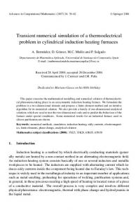
Figure 1.1: Coil windings of the LHC main bending magnet MB3004 after a quench at nominal current. The magnet developed an inter-turn short circuit which caused a meltdown of the cable and the cold bore (the tube separating the coil from the beam)[Walc 04, Siem 03].

[a] Quench [denotes] the uncontrollable and irreversible transition of a superconductor or a superconducting device from the superconducting state to the normal conducting state. With the development of a quench, several physically different but mutually dependent processes start: Due to the ohmic heating, the temperature increases and the normal conducting zone expands over the superconductor. If the device is short-circuited, the growing resistivity causes the current to decrease. The changing current results in a change of magnetic flux and thus induces eddy and magnetization currents in the metallic parts and cables, respectively. These induced currents create losses and additional heating, which distribute the normal zone even further. A quench poses two different threats to a superconducting device: high temperatures due to an unlimited ohmic heating, and excessive voltages due to a steadily growing resistance at high currents [Iwas 05]. High temperatures impair the electrical integrity of the insulation material or even cause a meltdown of the cable. Excessive voltages can result in an electric arc between adjacent coil windings punching holes into the insulation. In addition, the high current density and temperature gradients during a quench can cause an irreversible degradation of the current carrying capability of the superconductor. The violence of an uncontrolled electromagnetic discharge shall be illustrated by an incident which happened to the LHC main bending magnet MB3004 during cold testing on the test bench. During a quench at nominal current the insulation of the magnet failed [Walc 04] and the magnet developed an inter-turn short circuit. The excessive heat deposition in the short circuited turn caused a meltdown of the cable and the cold bore tube (the tube between coil and beam) [Siem 03]. The integrity of the cryogenic system was lost. Figure 1.1 shows the burnt-out coil windings after the incident. Superconducting devices, where the occurrence of a quench cannot be ex-

1.2 Quench Simulation cluded by the choice of operating conditions, need to be equipped with a protection system. The protection either relies on an intrinsically safe design or on active measures taken upon quench detection. In the former case, the device is designed such that it can withstand a quench without overheating and the quench is eventually able to recover. In the latter case, the current is extracted actively - as soon as possible - from the device by either increasing the internal resistance or switching in an external resistor. The design of the protection system is an essential part of the construction of any superconducting device. Therefore, quench simulation programs are needed in order to study the intrinsic quench behavior and define the necessary protection, to test protection schemes and to analyze measurement data.

1.2 Quench Simulation The simulation of quenches in superconducting magnets constitutes both, a multi-physics and a multi-scale problem. The accurate modeling consists of a thermal, a magnetic and an electrical network problem coupled by means of energy exchange and non-linear material properties. The required spacial resolution spans from less than a millimeter for the description of eddy currents in strands to several meters for an entire magnet. The involved time constants reach from some microseconds for the resolution of quench initialization to several minutes for the computation of full magnet ramp-cycles. The minimum energy required to quench part of a strand may be in the order of some micro joules while the total stored energy in a magnet ranges at several mega joules. Furthermore, quench computation constitutes a strongly non-linear problem. The relevant material properties, e.g. the thermal capacity and electrical resistivity, vary over many orders of magnitudes during a quench. In addition, superconducting materials exhibit hysteresis behavior. On this account, the simulation of quench on accelerator type magnets relies on the simplification of complex structures, homogenization of material properties, and analytical sub models. Consequently, any quench model is limited to a specific set of applications. This approach requires the coupling of several computation methods, e.g. finite-differences, finite elements, boundary-elements, Biot-Savart’s law, and network-models. The variation of material properties can be encountered by using an adaptive time-stepping approach or iteration methods. Quench models published in the literature mainly differ in their choice of simplification and their set of applied sub-models.

1.3 Literature Overview Quench codes Many calculation methods for quench in superconducting magnets have been published. Except for the very recent publication of Aird

3

4

Introduction [Aird 06], none actually aimed at the modeling of the entire multi-physics problem. Wilson published the computer program QUENCH [Wils 68] modeling the quench propagation due to ohmic heating in superconducting solenoids. A concept of field and temperature dependent, anisotropic quench propagation velocities is used to span the normal conducting zone over the coil. This approach was further developed by Rossi, first in DYNQUE [Cana 93] and later in QLASA [Ross 04]. A similar approach for accelerator type magnets can be found in [Laty 97] by Latypov. Krainz modeled and studied the protection of the LHC test string using an electrical network model [Krai 97]. The simulation of the current decay in a quenching magnet considering the external network, and a string of magnets based on the commercial software SABER was done by Rodriguez-Mateos [Rodr 97, Rodr 96]. Sonnemann and Calvi developed a finite difference model for the simulation of the quench propagation velocity based on thermal material properties and the local magnetic field called SPQR [Sonn 01b, Calv 00]. In [Sonn 01a] Sonnemann presented a quench model and quench measurements for magnets of the LHC. Kim published a finite difference model for the simulation of quench in [Kim 01]. The quench behavior of a superconducting undulator was simulated with a finite difference model [Bett 06] by Bettoni. Caspi and Masson presented thermal models for the quench simulation using commercial finite elements packages ANSYS [Casp 03] and COMSOL [Mass 07], respectively. The only program following an approach of hard-coupling of the different physical effects is the program of VECTORFIELDS [Aird 06]. Due to their focus on superconducting solenoids, with a huge number of fine windings, an individual winding scheme is not defined and turn-to-turn voltages can not be calculated. Sources on superconducting magnets and quench phenomenon In addition to the publications on quench simulation models, the following studies of the quench process have to be mentioned. Iwasa, Mess and Wilson address quench, relevant effects and quench protection in their books [Iwas 94], [Mess 96] and [Wils 83], respectively. Especially the book [Brec 73] of Brechna provides extensive material for the understanding of superconducting magnets and quench. Devred performed analytical quench studies for the SSC [Devr 89]. The thesis of Verweij provides valuable information on the stability of superconductors and on induced losses in superconducting cables [Verw 95]. Background for the presented work The work presented in this thesis builds on the CERN field calculation program ROXIE by Russenschuck [Russ 98]. The program provides all necessary functionality for the electromagnetic design of superconducting accelerator magnets including the numerical computation of the magnetic field produced by superconducting cables

1.4 Objectives of the Thesis and parts made from non-linear iron. In the past years, ROXIE has been extended to simulate field disturbances and losses stemming from inter-filament coupling currents (IFCC) [Wils 83], inter-strand coupling currents (ISCC) [Mari 04] and persistent superconductor magnetization currents [Voll 02]. Equipping ROXIE with an electrical network and thermal model allows for a coupled computation of all physical phenomena occurring during a quench.

1.4 Objectives of the Thesis The challenge of quench simulation is to model all relevant physical phenomena and effects with adequate accuracy, so that internal states of a quenching magnet can be reproduced and analyzed in order to understand the quench behavior. This leads to the following objectives: • Analysis of the quench process in superconducting magnets focussing on all physical effects and their relevance for the quench model. • Study and test of (existing) models describing relevant effects. Implementation and adaptation of the numerical models into a global computation environment. • Development of a quench algorithm: Study of the interdependence of the different sub-models. Implementation of a computational scheme reflecting computational cost as well as the necessary coupling between the sub-models. Finding a numerical method to resolve changes in material properties and time constants. The quench model has to be verified by reproducing measurement data with all material- and model-parameters chosen within the range of uncertainty. In a second step, the model can be used to extrapolate the magnet quench behavior to different initial conditions and slight design changes.

1.5 Structure of the Dissertation The dissertation is divided in three complementary parts, i.e. the thesis, the detailed treatment and the appendix. The thesis is structured in 4 main chapters: • Overview over features of accelerator magnets and physical phenomena occurring during a quench. We follow a typical quench process through a magnet and discuss the physical phenomena in respect to the magnet application. Definition of the scope for the quench model. • Introduction of numerical models for all relevant effects occurring during a quench. We give detailed explanations on the implementation and/or adaptation of the used sub-models and their internal states. The different models are weakly coupled in the quench algorithm and solved

5

6

Introduction by means of an adaptive time-stepping method. The such developed algorithm allows to study quench propagation, magnetic quench back, and voltages building up within the magnet winding. • Simulation results reproducing quench measurements from the LHC. The quench model provides a detailed view on the internal states of quenching magnets. The presented reproduction of the coil voltage signal including characteristic spikes clearly indicates the advantages of the coupled approach. • Extrapolation of the simulation results on new magnet designs and protection concepts. We show a detailed protection study for the LHC inner triplet upgrade. For the case of fast-ramping magnets we are exploring new protection possibilities. Moreover, we summarize the presented approach and obtained results. We give a critical analysis on aspects which could be subjected to further studies. In order to reduce the complexity of the main part, detailed treatments, e.g. common definitions and concepts of superconducting magnet design, derivations of electromagnetic models, and explanations of typical effects are collected in the last chapter. Notice that the different subjects are put down such that they can be read independently from the main parts. • Analytical hot-spot calculation by means of the MIITs-concept indicating the need for numerical methods. • Definition of the magnetic energy and the inductance in case of materials exhibiting hysteresis and diffusive behavior. • Derivation of the instantaneously dissipated hysteresis losses for the critical state model of hard superconductors. • Modeling Rutherford-type cables including induced losses. • Overview over magnet protection methods and voltages occurring during a quench. In order to provide the reader with all necessary information to reproduce the presented results the appendix contains the following sections: • Researched values are provided for all materials commonly used in superconducting accelerator magnets. We briefly review the physical background to all relevant material properties. • The definitions and formulae of model parameters describing the coil geometry. • Description of all magnets presented in this work. We describe all parameters of the superconducting strand and cable, the coil cross-section and iron yoke, the winding scheme and electrical network, as well as magnet protection.

2 Magnet Features and Physical Phenomena Dicebat Bernardus Carnotensis nos esse quasi nanos, gigantium humeris insidentes, ut possimus plura eis et remotiora videre, non utique proprii visus acumine, aut eminentia corporis, sed quia in altum subvenimur et extollimur magnitudine gigantea. John of Salisbury (1120 - 1180)

In this chapter we introduce relevant features of superconducting magnets and physical phenomena occurring during a quench. Due to the excessive requirements for the modeling of all physical effects, we have to reduce our approach and disregard a number of effects. The reduction is motivated by our application and briefly compared to other approaches.

2.1 Superconducting Magnets We distinguish between superconducting accelerator-type magnets and other superconducting magnets. The first are used to guide the beam of a particle accelerator on their orbit, i.e. bending them on a circular trajectory or focussing the beam. The latter kind comprises superconducting magnets for MRI, the LHC experiments ATLAS and CMS, as well as fusion projects like ITER. The typical design features of superconducting accelerator type magnets are introduced by means of the LHC main bending magnet. Major differences to other accelerator type magnets, e.g. superconducting correctors or superferric magnets, are discussed in the following. The section ends with a brief overview on the features of other commonly used superconducting magnets, e.g. solenoids, toroids, and undulators.

7

8

Magnet Features and Physical Phenomena

83("1-9/:3-;/0%@9'2%

!"#$%&'("%

)"#*%+,-.#/0"1%&'("%

)"2'3$455%6"77"2%

8(992%&'"-"%% !37%!#1%

83("1-9/:3-;/0%% !374!#1% 519/%7&'9*+%2' /#7*'9"#120,#%'56221'

Figure 2.4: Photo of the coil cross-section of the LHC MQY featuring the aperture, the insulation to ground including flaps, the coil protection sheet, the conductors, and the collar. Courtesy of G. Kirby CERN TE MSC.

Figure 2.4 shows a photograph of the typical cross-section of a superconducting accelerator magnet featuring the aperture, insulation to ground including flaps, the coil protection sheet, the conductors, wedges, and the collar. (Notice that lacking a photograph of LHC MB with comparable quality the LHC MQY is shown). Collars and iron yoke Consider the coil cross-section, the opposing currents of the two sides of the coil yield enormous electromagnetic forces pressing the coil apart. Therefore, the Lorentz forces are carried by a stiff collar made from non-magnetic material. Furthermore, the collar provides prestress to the coil preventing conductor movements. In the case of the LHC MB the two coils are accommodated in a common collar made of stainless steel. The iron yoke of a superconducting accelerator magnet serves two purposes: • Enhancing the field in the aperture without increasing the excitation current or the number of superconducting cables. Hence, increasing the efficiency of the design. • Reducing the magnetic field outside the magnet, i.e. the fringe field, in order to provide safe operating conditions for electronic equipment in close vicinity. In the case of the LHC MB, the iron yoke accounts only for 3% of the magnetic induction compared to an iron free design [Evan 09, p. 75]. However, the iron yoke reduces the stray field outside the iron yoke to less than 50 mT [Russ 07, p. 391]. Both, collar and iron yoke, are stacked in order to reduce induced eddy current losses. In the case of the permeable iron this results in an anisotropy.

12

Magnet Features and Physical Phenomena Helium-II vessel and heat exchanger The coil, the collar and the iron yoke are immersed in liquid helium II at 1.9 K. Helium II features an extremely low viscosity and percolates every cavity inside the coil windings and the stacked collar and iron yoke. The heat exchanger pipe provides a heat sink. The helium-II vessel is made of the shrinking cylinder on the outside, the beam pipe on the inside and the end caps. The liquid helium is filled in to the vessel via the bus-bar pipes. The helium-II vessel is wrapped in superinsulation blocking heat radiation and placed in a vacuum cylinder preventing convective heating. Magnet protection and external network In case of a quench the magnet needs to be protected from excessive voltages and temperatures. A quench needs to be detected as soon and reliably as possible and the current has to be extracted as fast as possible. During operation the differential voltage over the two apertures is measured and compared to a given threshold voltage. When the voltage exceeds the threshold and the reading has been verified after a predefined delay, a quench is detected. The LHC MB is operated in strings of 154 dipoles all connected in series. A current controlled power supply is setting the current in the string. In case of a quench, the power supply is switched off and by passed by a free-wheeling diode. A dump resistor is switched into the circuit in order to extract the current. A bypass diode is mounted inside the cryostat of every magnet. After quench detection the quench heaters of the quenched magnet are fired. The resistive voltage switches the by-pass diode and the magnet current begins to commutate into the diode. Hence, the magnet disconnects from the rest of the string allowing for a faster current decay. Bus bars The connection terminals of the dipoles are on one side of the magnet. For the series connection of the string of magnets the bus bar is placed within the cryostat on the outside of the iron yoke. The cryostat of the dipoles further more hosts small superconducting corrector magnets and their powering, as well as the current leads for the main quadrupoles.

2.1.2 Other Magnet Types and Design Features Design features less pronounced or relevant for the LHC main dipoles are introduced by means of other magnet types. Due to the wide variety of applications and technical solutions, this list is in now way complete, nevertheless, will give the necessary overview. Corrector magnets In order to compensate for field errors of the main bending and quadrupole magnets, and for the correction of particle offsets, corrector magnets are incorporated into the accelerator ring. The design of corrector magnets ranges from spool-pieces, small superconducting multipole magnets

2.1 Superconducting Magnets wound from a single wire and placed on the beam pipe, to double aperture magnets of a few meters. In the most basic design, the corrector is operated well below the critical surface, leaving enough margin to withstand probable disturbances [Evan 09, p. 76]. For the case of a quench, the magnets are provided with a parallel resistor taking over the current as soon as the quench has grown wide enough. Winding the coil with a single wire results in a significantly higher inductance. Super ferric magnets The design of super ferric magnets is based on the same principles as for normal conducting magnets. The magnetic field is concentrated and formed by a ferromagnetic iron yoke in the center of the coil. Instead of water-cooled copper cables the coil is wound from superconducting cables. Owing to the high available current densities in superconductors and the domination of the field quality by the iron yoke, super-ferric magnets can be made with a small number of winding turns. It is possible to use cable-in-conduit conductors; superconducting filaments inside a metal tube cooled by a constant flow of liquid helium. The superconducting coil is hosted in a cryostat mounted inside the iron yoke. With additional cooling, the magnet can withstand higher losses and be subjected to faster current ramps. Block-coil and double pancake Alternatively to coils designed following a cos θ-approximation, in the block-coil or double pancake design, the coil cross section consists of rectangular blocks arranged around the aperture. Figure 2.5 shows a sketch of three non-accelerator type magnets: a toroidal coil, a solenoid, and an undulator. Notice that all three magnet types are based on completely different topologies and frames of reference. Hence, they require a different description and calculation method. Solenoid Superconducting solenoids can be wound from a single strand (MRI) or a Rutherford-type cable (CMS). In the first case, the coil features large number of windings and consequently a high inductance. Such systems may be subdivided to steer the field quality or for quench protection. All sub-coils are provided with a bypass diode or shunt resistor constituting a inductively coupled system. Winding the solenoid on a conductive central cylinder yields a coupled secondary coil providing resistance and heating during a current ramp or quench. In the case of CMS, the cable used for the solenoid is surrounded by highquality aluminum (many times the cross-sectional area of the cable) in order to provide mechanical stability as well as a parallel path in case of quench. Superconducting Undulator Equipping an undulator with superconducting coils allows to operate with much higher current densities compared to copper

13

14

Magnet Features and Physical Phenomena

!"#

%$+,-.$%% !/$#(),0% '#()#(*&%

1"2,%

!"#$&%

Figure 2.5: Sketch of other superconducting magnet configurations: part of a superconducting undulator featuring an iron yoke and two and a half poles, solenoidal coil wound on a metallic cylinder, and a toroidal coil configuration.

coils. Nevertheless, the poles of the iron yoke saturate completely and the field is mainly created by the coils [Hila 03]. The coils of the different poles may be connected in series and by-passed by diodes, or powered individually. In both cases, the current profile in all coils are coupled by the non-linear mutual inductance of the iron yoke. Toroids In toroidal systems as for ATLAS or ITER, every coil is hosted in its own cryostat. The cable-in-conduits can be used for the windings allowing to cool effeciently. The coils are magnetically coupled.

2.2 Quench Process The various physical effects occurring during a quench in a superconducting magnet are introduced following a typical quench in one of the LHC main bending magnets. Subsequently, we refer to other relevant phenomena. Quench cause A superconductor quenches when the working point defined by the local magnetic induction, the current density, and the temperature exceeds the critical surface. The temperature difference between the working temperature and the maximum temperature for the given field and current Temperature density is denoted temperature margin; the conductor quenches for zero margin: margin. Sec. 7.1 A temperature increase in the magnet can be caused by conductor movements and the associated friction, induced eddy current losses in the superconducting cables, radiation and beam particles entering the coil, quench heaters and heat transfer from adjacent conductors. The current density in the superconducting cables consists of the current provided by the power supply and the current driven by the induced voltages. Both can result in a quench in case of an over-current. Figure 2.6 summarizes the different phenomena leading to a quench. For accelerator magnets we can distinguish the following types of quench [Mess 96, p. 119]: Critical Surface: Sec. A.2

2.2 Quench Process

,(7'%(,) /#&(,75,)

2#$%&,$)+"4'7A,) !%((,#')+7(/70"#)

!%((,#')) /#&(,75,)

?@',(#74)C,4$5)

B/,4$)/#&(,75,)

?@&,,$/#A)&(/0&74)5%(.7&,)

;,7')$,>"5/')

!"#$%&'"()*"+,*,#')-.(/&0"#1) 2#$%&,$),$$3)&%((,#')4"55,5) 67$/70"#) 8,7*)4"55,5) 9%,#&:):,7',(5) ;,7') 0  0 ij (3.5) INC = IM − Icij (∆Jcij = 0) & (Icij > 0),   IM else where IM denotes the current through the conductor and Icij the critical current in the element for a the local magnetic induction and temperature: i Icij = Jc (Bpeak , T ij )Aicab,SC .

(3.6)

3.3 Magnetic Field Model !"

!!'

$"

=:>?(':$9;8B$796C7$/'' D:$7$'' !(*$/%+'0'!!','-'

Figure 3.3: Current sharing: The transition from superconducting to normal conducting state can be subdivided into three phases. During the first$.& phase, the conductor current (*$/%+0&','-' is carried by the superconductor (ISC = IM ). The temperature in the conductor increases only due to external heating or induced losses. The critical current in the conductor decreases due to the increase of temperature. The second phase begins, when the critical current drops below the conductor current and the excess current spills over into the normal conducting part (ISC + INC = IM ). The conductor is considered in the quenched state. !"#$%&!"##$%&'()#*%+, Ohmic heating in the normal conductor amplifies the temperature increase. The last phase is reached, when the critical current has decreased to zero and the entire current is carried by the normal conductor (INC = IM ).

ij Only the current INC flows through the resistance of the element ij and therefore causes ohmic heating. The conductor current IM flows entirely in the normal conducting matrix as soon as the critical current is zero, i.e. the critical field is zero. Figure 3.3 shows a schematic of the current transition including current sharing.

3.3 Magnetic Field Model Assuming that the magnet is long compared to the diameter of the magnet cross-section, which is generally true for dipole- and quadrupole magnets in accelerators, an 2D approach is used for the magnetic field calculation. The magnetic field problem can be divided in 3 sub-domains, i.e. the superconducting coil, magnetic materials as for the iron yoke, and empty space, e.g. the beam pipe. The coil consists of superconducting cables which are subjected to eddy currents and magnetization effects. The quench model relies on the peak and average magnetic induction as well as on the average magnetic vector potential on all conductors. Assuming that induced eddy currents are small compared to the transport currents their contribution to the magnetic induction is not taken into account. Therefore, the field computation consists of the following two steps: 1. Calculation of the field created by the currents in the coils. 2. Computation of the secondary field of the magnetic materials as repercussion on the coil field.

26

Numerical Modeling +"#,%&'()*$

!1&).$

!"#$%&'()*$

!1&).$ !"

-&).$ /()0$

!)0&*$

/)0&*$

Figure 3.4: Magnetic field computation: The problem is subdivided into the coil, an iron and an air domain. The magnetic induction B is composed from the field of the coil and the field of the iron domain.

The solution of both steps are iterated due to the field-dependent permeability. Figure 3.4 shows the subdivision of the magnet and the field calculation at an arbitrary position relying on coil and iron field. The total field is used for the computation of the cable eddy currents and magnetization, and the consequent losses.

Rutherfordtype cable: Sec. 7.8

Coil fields The magnetic field of the superconducting coils is calculated from the field of ideal line currents. The cross-section of any conductor is evenly subdivided into NDis patches, shown in Fig. 3.5 (left). Outside the cable, more precisely outside any strand, the magnetic field is given by the sum over the fields of the line currents placed in the center of the patches, rik . If evaluating the field inside a strand, e.g. for the calculation of peak fields on a conductor, the respective line current is replaced by a homogeneous, cylindrical current distribution and singular expressions are avoided, see Fig. 3.5 (right). The transposition of the strands along the axis of Rutherford-type cables is not taken into account. Magnetic Materials The influence of magnetic materials on the magnetic field in the coils is calculated by means of the BEM-FEM-coupling method. According to this method only domains containing magnetic materials are meshed and described by means of finite elements (FEM). Empty space and more relevant the coils are not modeled in finite elements but considered by expressing the magnetic field on the boundary to the iron/FEM domain. The field repercussion of the magnetic materials on the coil fields is calculated using a boundary element approach (BEM). For field-dependent magnetic permeability (iron saturation) the coupling between the two domains is solved iteratively. The BEM-FEM approach reduces the necessary number of finite elements significantly. Furthermore, coil fields can be modeled more precisely and independently of the used mesh. Differences of the magnetic permeability, as shown in Sec. A.1.6.1 between

3.3 Magnetic Field Model !"

#"

#"

#"

#"

#"

#"

27 !"

$"$" !" #"

$"&'($"

!"

!!"#"

%%"

$"%()$" $"

Figure 3.5: Calculation of the field of a conductor. (left) Discretization of the conductor *+,&-.#$%&'()$!*+,(!-./0.$%12-034+-5&6 i. The index k denotes the patch number. (right) Peak field calculation. The field inside a strand (shaded) is given by the field of all line currents, Bext , plus the field of the homogeneous cylindrical current distribution inside the strand, Bstr .

various operation conditions and manufacturers, are negligible for the calculation of quench relevant quantities, i.e. for coil fields and the inductance.

Total magnetic induction - Superposition The magnetic induction as well as the magnetic vector potential at any of the positions rik is given by the sum of all field sources. In the present work only the coil field and the iron repercussion are considered, thus Bik

=

X

Bmodel (rik ) = Bcoil (rik ) + Biron (rik )

(3.7)

Amodel (rik ) = Az,coil (rik ) + Az,iron (rik )

(3.8)

model

Aiz,k

=

X model

Discrete field quantities For the present work two different cable types are considered: Ribbon-type and Rutherford-type cables. The strands of a Rutherford-type cable are twisted along the cable axis, i.e., every strand of the cable takes every position within the cable cross-section over the twistpitch length. With a twist-pitch much shorter than the magnet length, the magnetic field varies only over the cross section but not along the conductor. Therefore each strand is exposed to the full variation of the field. For the calculation of material properties the average field is used as discussed in Sec. 7.8. For the calculation of field dependent material properties, e.g. magnetoresistivity and specific heat of superconductors, the average modulus of the field on the conductor is required. The quench decision depends on the peak

Cable types: Sec. B.1.3

28

Numerical Modeling field on the conductor: Biav

=

i Bav

=

i Bpeak

=

i PNDis

i k=1 Bk , i NDis i i PNDis k=1 Bk , i NDis i max{ Bk }k=1,...,N i , Dis

(3.9) (3.10) (3.11)

The average magnetic vector potential in conductor i is used for the calculation of linked fluxes and induced voltages, i PNDis i k=1 Az,k i Az,av = . (3.12) i NDis We can assign a local frame to every conductor cross-section by defining a vector parallel, e|| , and orthogonal, e⊥ , to the broad face. For keystoned cables the parallel vector is approximated by the cable center as indicated in Fig. 7.20. We define the average magnetic induction parallel and orthogonal to the broad face as: B||i = Biav · e|| , Magnetic length

i B⊥ = Biav · e⊥ .

(3.13)

Although the variation of the magnetic field in the coil ends is not directly taken into account for the computation of losses or material properties, it has to be considered for the computation of induced voltages and the differential inductance. In Sec. B.1.6, three different coil lengths are introduced, the winding length `w , the magnetic length `mag and the inductance length `ind . Comparing the inductance per length as well as the inductance of a magnet measured or calculated in 3D gives the inductance length. For the calculation of induced voltages over elements the factor `ind `w is used to scale the longitudinal extensions. kmag =

(3.14)

3.4 Induced Losses Cable eddy currents: Sec. 7.6

Hystersis losses: Sec 7.7

Eddy-current losses in the cable are calculated from the local field sweep. We distinguish inter-filament (IFCC) and inter-strand coupling currents (ISCC). Interfilament coupling currents are induced in the twisted superconductorcopper matrix of a strand. Inter-strand coupling currents are induced in a Rutherford-type cable in loops of superconducting strands and contact resistances between strands. The two phenomena are summarized as cable magnetization, see Sec. 7.6. Superconductor magnetization hysteresis losses are disregarded as discussed in Sec. 7.7. Eddy currents in copper wedges between coil blocks and in coil collars are not taken into account.

3.5 Electrical Network

29

Analytical magnetization losses Consider a Rutherford-type cable consisting of Nsi strands. The loss density for a time-variant magnetic induction are given by Eq. (7.63). Since every strand is fully exposed, the average loss per strand can be calculated from the average magnetic induction over the cable cross-section. The inter-filament coupling losses dissipated in the cable are then given by i i (3.15) piIFCC,av , = Ve,str PIFCC i where Ve,str denotes the volume occupied by the strands in any element of the conductor i. The inter-strand coupling loss density calculated from the average magnetic induction as given in Eq. (7.68). We get: i i PISCC = Ve,str piISCC

(3.16)

In case of a quench the ohmic heating over the resistive zone, exceeds the induced losses. Furthermore, the loss models are based on the assumption of superconducting filaments and strands. Therefore, induced losses are only taken into account while an element is in the superconducting state. The total losses in one element are calculated from the sum of different loss models ( i i PIFCC + PISCC ∆Jcij > 0 ij P0,losses = (3.17) 0 else Time dependence The analytic loss models are lacking the diffusive process, i.e. the losses are an immediate response to any field change. In order to avoid an over estimation, the coupling-current time-constants τlosses is a user supplied parameter. The total losses are given to    t − tfc ij ij , (3.18) Plosses = P0,losses 1 − exp − τlosses where tfc denotes the instance of the last field change. Notice, for the quench algorithm it can be required to split the time interval τlosses over several calculation steps. The steady continuation of exponential decays is shown in Sec. 7.5.2.

3.5 Electrical Network The magnet is connected to an external network represented by an generic network model as shown in Fig. 3.6. It consists of a power supply, an energy extraction system with switch and dump resistor, and a serial resistance and inductance. The power supply is bridged by a free-wheeling diode in order to conduct the current after it is switched off. The serial elements can represent resistive current leads and the inductance of magnets connected in series to the magnet. The magnet itself is represented by its electrical resistance and

30

Magnet protection: Sec. 7.9

Sequence of events: Sec. 7.9.6

Numerical Modeling the differential inductance. It can be bridged with a parallel resistor or a by-pass diode. This generic electrical network allows to simulate quenching magnets in single operation, e.g. on a test bench, or in a string, e.g. as for the main dipoles in the LHC tunnel. Both configurations are explained in Sec. 7.10.1 and in Sec. 7.9 in respect of quench protection. The by-passing of the quenching magnet is explained in Sec. 7.9.3. The generic approach allows only to simulate one current in the magnetic system. Therefore it does not permit to simulate quench protection by magnet subdivision or a coupled secondary winding (see 7.9.4). Quench detection and validation A quench is detected as soon as the resistive voltage over the magnet Ures exceeds the detection threshold voltage Udet . The quench is validated, if the resistive voltage remains above the threshold level after a discrimination time ∆tDis . Quench protection measures are triggered after quench validation, t = tval . The numerical simulation automatically distinguishes the induced and resistive voltage over the magnet. Therefore, compensation methods as described in Sec. 7.9.1 are not required. Nevertheless, it is possible to monitor and use any voltage within the magnet windings for quench detection. Current change The generic electrical network model can be described by means of three currents: the current through the quenching magnet IM , the current through the by-pass diode ID and the current in the main circuit IE . The current through the power-supply commutates instantaneously into the free-wheeling diode after switch-off and therefore does not require the definition of a fourth independent current. The three currents are related by IE = IM + ID .

(3.19)

The underlying mechanism of current decrease in the three branches, changes with the switching of the two diodes. While the power supply is connected to the network, the current function IPS (t) is imposed, i.e. IPS = IM = IE . Quenching of the magnet or switching of the dump resistor show no effect. The current change is given by, dIM dIPS dIE = = , dt dt dt

dID = 0. dt

(3.20)

After the power supply is disconnected, the current decrease is defined by the main circuit (IE = IM ) and yields   R + R Q s IM + UDR + UfDf dIM dID dIE = =− , = 0. (3.21) dt dt Ld + Ls dt When the terminal voltage UTerminal reaches the threshold voltage of the bypass diode, the magnet current starts to commutate into the parallel path.

3.5 Electrical Network

31

34#"+56"%'7*%"#)'

!3'

#8'

"$#/'

"6"8'

.#$6*:'!:#0#")/'

$7'

!/'

!"#$%&'!()$*+,-"'.&/)#0'

#/' !12' "12'

"9#$06"*:' $1' *//'16-8#'

"+1;' $!'

";1;' "?.'

A$##=@5##:6"%' 16-8#' ?-@#$'.4>>:&'

Figure 3.6: Generic electrical network model: Quenching magnet, energy extraction 7-8#:B!"#$%&'$(")#%*+&,system with dump resistor and switch, power-supply with free-wheeling diode, and serial elements. The magnet is represented by the resistivity of the quenched conductors and its differential inductance. It can be bridged with a parallel resistor or a diode.

The current decrease in the main circuit thus depends only on the serial inductance. dIE dt dIM dt dID dt

UfDf + UcDf + UDR + Rs IE , Ls RQ IM − UcDf = − , Ld dI = − M. dt

= −

(3.22) (3.23) (3.24)

If no serial inductance is present, the current in the main loop IE drops to zero instantaneously. For a string of magnets, where the total inductance is orders of magnitude larger than the inductance of the quenching magnet, protected by means of quench heaters, the main current IE can be considered as constant (see Sec. 7.10.1).

3.5.1 Lumped Network Elements Power supply In the absence of a quench, the magnet current is imposed by the power supply. The current ramping IPS (t) is determined by the magnet operating conditions. The voltage over the power supply is controlled such that the current change follows the specifications. This compensates for the non-linear inductance and the resistive components in the circuit, i.e. resistive joints or a quenching magnet. After quench validation, the power supply switch-off is delayed by ∆tQT . The current commutates instantaneously into the free-wheeling diode.

Numerical Modeling #!% # 0. For loss and hysteresis free materials we obtain an alternative form for the stored magnetic energy: A1 Z Z A1 ∞ J · dAdV (7.25) Wmag = A0

VJ

A0

7.4 Inductance The magnetic flux in a superconducting magnet is in non-linear, diffusive and hysteretic relationship with the applied current due to iron saturation, induced eddy currents and superconductor magnetization. For the simulation of quench, the electrical circuit is represented by lumped elements and the current change in the loop is calculated from the voltage over the inductance. Therefore, the inductance is derived for general materials and then applied to quench computation.

7.4.1 Self Inductance Consider a simple current loop connected to a current source as shown in Fig. 7.8. The loop spans a surface A with differential surface element da and boundary ∂A. The differential line segment ds follows the boundary in a right-hand orientation. The total magnetic induction B consists of the field created by the current I and the effect of any magnetic object with field-dependent, diffusive or hysteretic properties. The dependence of the magnetic induction B on Rt the current I, the current change ( dI ) and the current history ( I dτ ) is dt t0 modeled by the relation Γ,    Z t dI B = B r, Γ I, , I dτ . (7.26) dt t0 For the general case, the following, commonly used equations give rise to the definition of three different types of self inductance [Kurz 04]. Ψmag = LΨ I,

Uind = Ld

dI , dt

Wmag =

1 L I 2. 2 W

(7.27)

In the stationary case, with constant material properties and no hysteresis, all three inductances are identical: LΨ = Ld = LW . Apparent inductance: For a given instance and current, the magnetic flux ΨA mag through the surface A is given by Z Z ΨA = B da = A · ds, (7.28) mag A

∂A

94

Detailed Treatment !"

!#"

!" !$"

!"

#"$#$

Figure 7.8: Self inductance geometry. The current loop with surface A and boundary ∂A. The differential line segment and surface element are denoted da and ds, respectively.

where A denotes the magnetic vector potential with ∇×A = B. The apparent inductance [Deme 99] LΨ is defined by LΨ =

ΨA mag

R =

I

∂A

A · ds . I

(7.29)

The magnetic flux shows the same dependence on the current as the magnetic induction. With the limitation to a constant current, i.e. a steady state situation, the apparent inductance may be non-linear and hysteretic. Differential inductance: Assuming a current ramp-rate dI dt , the voltage induced over the terminals of the current source, Uind , is given by Uind =

dΨA mag

=

dt

d dt

I ∂A

A · ds =

I ∂A

∂A · ds, ∂t

(7.30)

and defines the differential inductance Ld [Naun 02, pp. 33] to: Ld =

Uind dI dt

=

dΨA mag dt dI dt

=

d dt

H

A · ds

∂A dI dt

.

(7.31)

The differential inductance inherits the behavior of the magnetic induction and may generally be non-linear, time-dependent and hysteretic. dΨA

dΨA

Under the condition that dtmag = dImag dI dt , i.e. that the system is timeinvariant, non-hysteretic and does not contain any secondary loops, the definition can be further simplified to: Ld (I) =

dΨA mag dI

=

d (ILΨ ) dLΨ = I + LΨ . dI dI

(7.32)

Notice that a second current loop, which is magnetically coupled to the primary loop, would influence the induced voltage, but has no effect on the apparent inductance.

7.4 Inductance

95

Energy inductance: For a system in virgin state, i.e. current and all fields equal zero, the current is changed to I(t). The amount of energy Wsource supplied by the power supply can be calculated from Z t Z t dΨA mag (I(τ )) Wsource (t) = Uind (τ )I(τ ) dτ = I(τ ) dτ. (7.33) dτ τ =0 t=0 Note that only for a loss and hysteresis free system, the energy supplied by the source and the magnetic energy stored in the system are identical. The energy inductance LW is then defined as time-dependent function: LW (t) =

Wsource (t) 2 = 2 1/2I(t) I(t)2

t

dΨA mag (I(τ ))

t=0

dτ

Z

I(τ ) dτ.

(7.34)

Under the following two conditions the expression for the energy inductance dΨA

(I)

dΨA

(I)

mag mag dI can be further simplified. If again = dt dI dt , then the time derivative can be split off. If the system is conservative, i.e. the energy change does not depend on the current history, but only on start and end current, then Eq. 7.34 reads: Z t dΨA 2 mag (I(τ )) dI LW (t) = I(τ ) dτ (7.35) 2 I(t) t=0 dI dτ Z I(t) dΨA 2 mag (I) = I dI (7.36) I(t)2 I=0 dI Z I(t) 2 L (I)I dI (7.37) = I(t)2 I=0 d

From the energy inductance the concept of inner and outer inductance can be derived. Using the formula for the magnetic energy inside a volume V , Eq. (7.20), the energy can be calculated separately inside and outside the cable. Both energy fractions define complementary parts of the total induction. For materials with constant properties where all three concepts of induction are identical, the two parts can be conveniently approximated: The outer induction is calculated from the geometrical induction of a loop along the conductor. The inner inductance is given by the inductance per unit length of a straight infinite long wire with the same cross-section multiplied by the length along the loop.

7.4.2 Mutual inductance Consider a second current loop of surface B and boundary ∂B. Surface and boundary can be parameterized by da and ds, respectively. The two surfaces A and B do not intersect. Both loops are magnetically coupled, i.e. the flux of loop A penetrates loop B and vice-versa. The geometry may contain magnetic objects with field-dependent, diffusive or hysteretic properties. The concept of the geometrical and differential inductances are adapted to the new situation:

96

Detailed Treatment Apparent mutual inductance : For a given current I = IA in loop A and IB in loop B, the apparent mutual inductance of B on A, is given by relating the magnetic flux created by B in loop A to the current IB : AB MΨ =

ΨA mag IB

H =

∂A

A · ds . IB

(7.38)

In general, the magnetic flux depends on both currents, i.e. on ΓA and ΓB and so does the apparent mutual inductance. If the material properties are constant, the flux can be separated into the contributions of either coil. The AB BA apparent mutual inductance is then constant and symmetric, MΨ = MΨ . Note that symmetry is not easy to define in case of varying material properties when the mutual induction is given by a function. Differential mutual inductance: The current in loop A shall be constant IA . The voltage induced over loop A due to loop B is now related to the current change in loop B: MdAB

=

A Uind dIB dt

=

dΨA mag dt dIB dt

=

d dt

H

A · ds

∂A dIB dt

(7.39)

7.4.3 Application of the Differential Inductance to Quench Computation Since magnet components may be build from field-dependent, diffusive and hysteretic materials the general definition of the differential inductance given in Eq. (7.31) is applied. Bulk or Rutherford-type conductors For a current loop made from a bulk conductor, the confined flux varies over the conductor cross section. Isolating the average linked flux, yields a differential flux over the cross section giving rise to eddy currents. The change of the average flux induces a voltage over the loop terminals (see Fig. 7.9 (left, center)). For a Rutherford-type cable, all strands are connected in parallel and follow a zig-zag trajectory along the cable (see Sec. 7.8). The linked flux on all parallel paths is identical and the total induced voltage can be calculated from the average inductance. The variation of the differential electrical field along the strands also gives rise to induced eddy currents - inter-strand-coupling currents (see Fig. 7.9 (right). Field-dependent materials The permeability of the iron yoke is field dependent and decreases strongly as soon as the magnetic induction exceeds the saturation level. Therefore, the contribution of the iron yoke to the flux in the magnet decreases with increasing current. If no other dependence needs to be considered it can be shown that the differential inductance is smaller

7.4 Inductance

97 !"#

%$!#&% '!%

'!% !#&%

Figure 7.9: Inductance of a bulk or Rutherford-type conductor. (left) and (center, bottom) The confined flux varies over the conductor cross section. (center, top) The induced electric field can be split in a an average and differential part. (right) The average induced electric field is identical for each strand. The differential electrical field gives rise to induced inter-strand eddy currents.

or equal to the geometrical inductance. Compare Eq. (7.32) where the flux change with current is negative. Notice that the magnetic field computation is carried out entirely in 2D, i.e. over the magnet cross-section. The variation of the magnetic field in the coil ends and the magnetic length are taken into account by scaling parameters. For the induced voltages the magnetic length `mag is used (see discussion of magnetic length and inductance length in Sec. B.1.6). The iron saturation is different in the magnet ends. Hence, the magnetic length is a function of excitation current. Figure 7.10 shows the differential inductance for the LHC main bending magnet considering saturation effects in the iron yoke.

The influence of induced eddy currents and superconductor magnetization on the differential inductance are not taken into account in the present quench model. Nevertheless, the general dependence is discussed allowing to analyze peculiarities of inductance measurements. Diffusive materials Induced eddy-currents or inter-strand coupling currents show a diffusive characteristic. The influence on the differential inductance is estimated by means of a simple network representation [Smed 93]. The induced eddy-currents are considered as coupled secondary loops. The magnet is represented by the primary side of a transformer with inductance L1 . The sum of all inter-strand and inter-filament coupling currents is taken into account by a secondary circuit with inductance L2 and p resistance R2 . The two sides are coupled by the mutual inductance M = k L1 L2 , where k is denoted the coupling factor, k[0, 1). The inductances L1 , L2 and M are constant. At t = 0 a constant voltage U1 is switched over the magnet.

7.1

12

7

10

6.9

8

6.8

6

6.7

4

6.6 6.5

Magnetic Iron (MI) MI + Persistent Currents Current 0

300

600

900

1200 Time in s

1500

1800

2100

Current in kA

Detailed Treatment Differential Inductance per unit length in mH/m

98

2 0 2400

Figure 7.10: ROXIE simulation of the differential inductance of the LHC main bending magnet considering field dependent and hysteretic materials. The differential inductance only considering the field depending iron decreases by approximately 5% from injection to nominal current. Considering persistent currents (hysteresis), the differential inductance shows a significant dip after the current ramp-rate changed sign (at t = 0 and t = 1200 s, assuming a pre-cycle for t < 0).

For a symmetrically oriented transformer (see e.g. [Flei 99, p. 494]) the current in the secondary winding is given by    U M L t i2 (t) = − 1 1 − exp − (7.40) , τ = 2 (1 − k 2 ). R2 L1 τ R2 Calculating the differential inductance from the induced current change on the primary side yields, Ld (t) =

U1 di1 dt

= L1

1+

k2 1−k2

1
exp − τt

(7.41)

The time constant and the initial value of the inductance are both simple functions of the coupling factor k. Figure 7.11 shows the change of differential inductance for different values of the coupling factor. It can be seen how the differential inductance is reduced in the first instance after the voltage rise. Hysteretic materials: In superconducting magnets the magnetic iron and the superconducting filaments show a magnetization behavior which features a hysteresis. The influence on the concept of the differential inductance is highlighted by means of a simplified model. Figure 7.12 (top, left) shows the magnetic flux stemming from the hysteretic material in the magnet versus applied magnet current. The transition from the lower to the upper branch as well as the shape of the minor loop are typical for the superconductor magnetization. In case of ferromagnetic hysteresis, the

7.4 Inductance

99

1.0 0.5

0.8 Ld !L1

0.0 0.25

0.75

0.6 0.4

0.9 Τ0.75

0.2 k ! 0.99 0.0 0.0

0.2

0.4

0.6

0.8 t ! "L2 !R2 #

1.0

1.2

1.4

Figure 7.11: Differential inductance of a magnet with time-transient effects, e.g. interstrand coupling currents. The plot shows the change of differential inductance over time for different values of k: On the left we can read off the initial value. The time constant τ corresponds to the ending of the full lines.

%&'($

%&'($ !"

%"

$!"#$ #"

!"

#" Figure 7.12: Differential inductance by means of hysteretic materials. The hysteresis loop represents a simplified superconductor magnetization loop including a minor loop. Starting from the current, the magnetic flux in the magnet can be constructed by a simple projection. The induced voltage is given by the flux change. Finally, the differential inductance is calculated from the ratio of induced voltage and current ramp rate.

100

Detailed Treatment transition occurs while increasing the current as compared to superconducting materials where the transition occurs on the on-set of the current decrease. Minor loops are followed horizontally instead of vertically. Following the approach used in [Naun 02, pp. 36], the flux in the magnet can be constructed graphically from the applied current. The flux belonging to the geometry of the magnet winding is not considered here. The induced voltage is calculated from the flux change. Both are shown in Fig. 7.12 (top, right). For this simplified model, the differential inductance is constant and negative during the branch transition and zero everywhere else. In case of ferromagnetic materials, the differential inductance is of constant positive values during the transition (which occurs at different times). In first order, this effect can be superimposed on the geometrical inductance and thus yields lower/higher values during the transition. Figure 7.10 shows the differential inductance for the LHC main bending magnet considering the effect of superconductor magnetization currents.

7.5 Non-linear Voltage-Current-Characteristic of Superconductors Non-linear VAC

Current controlled voltage source

The voltage-current-characteristic (VAC) of a superconductor is a strongly non-linear function of applied magnetic field, temperature and current (or current density), see Sec. A.2.2. Following Wilson [Walt 74, p. 30], the voltage over a superconductor, USC , can be expressed by a power of the applied current ISC , NSC  ISC , (7.42) USC = Uc Ic where NSC serves as fit parameter and Uc as reference voltage (Sec. A.2.3). The critical current Ic depends on the applied magnetic field and temperature (see critical current density in Sec. A.2.4). In an electrical network, superconducting elements constitute current-controlled voltage sources, USC (ISC ). Therefore, branch currents and voltages cannot be determined by a simple inversion of the network matrix, but require a (numerically expansive) iterative approach to resolve the interdependence (non-linearity). Consider the combination of a superconducting and a resistive element in one branch of a simplified electrical network as sown in Fig. 7.13. Depending on the type of connection, in parallel or in series, and the boundary condition, current or voltage driven, four different elementary problems can be derived: a) superconductor in parallel to a resistor driven by a current source: The current splits over the two branches, the current through the superconductor defines the voltage over the branch and thus the current through the resistor. This situation is called current-sharing and represents the situation of a quenching copper-stabilized wire, see Sec. 7.5.1.

7.5 Non-linear Voltage-Current-Characteristic of Superconductors '

%$!&"%

$&"%

($% !%

!" !!"% )

%$#!"#!!"$% #"

!&"%

$&"%

#!"#!

%$*

%$$&"%

#" !!"%

!!"%

#!"#!!"

%$$&"%

#!"#!!"

%$Figure 7.13: Simplified electrical networks containing superconducting and normal con+,,-.*/01233'431&5.6/.-'78-9':/571!"#$#% ducting elements. The following situations can be identified: a) Current-sharing or the voltage over a quenching copper stabilized wire. b) Voltage over a partly quenched magnet winding. d) Voltage over superconducting current loop with resistive joints. The subscripts “NC” and “SC” stand for normal conductor (ohmic resistive) and superconductor, respectively.

b) superconductor in series with a resistor driven by a current source: The current through both elements defines the total branch voltage. This situation can be found in case of partly quenched magnet windings. c) superconductor in parallel to a resistor driven by a voltage source: The voltage over the branch defines the two branch currents. d) superconductor in series with a resistor driven by a voltage source: The voltage over the branch splits over the two elements. The voltage over the superconductor defines the branch current and therefore the voltage over the resistor. This situation can be found for induced voltages over superconducting loops with resistive joints, see Sec. 7.5.2. While the situations b) and c) are easily solved and implemented, the circuits a) and d) require either further simplifications, iteration techniques or a graphical solution (Sec. 7.5.3).

7.5.1 Current-Sharing Superconducting filaments are usually embedded in a normal conducting matrix for stabilization. The matrix gives mechanical support, heat transfer to the coolant and in longitudinal direction along the strands, and provides a parallel path for the current in case of a quench.

101

102

Implicit equation of currentsharing

Detailed Treatment Such a superconducting strand can be described by the circuit shown in Fig. 7.13 a). While the current is much smaller than the critical current Ic , the voltage over the superconductor is negligible due to the usually large n-index (in the order of 20-50). For an increasing current I or a decreasing critical current Ic , e.g. due to a temperature or magnetic field increase, the voltage USC , given in Eq. (7.42), starts to grow. This voltage draws part of the current into the path through the resistor - the external current I is shared between the resistive and superconducting path. Neglecting the inductive coupling of the two current paths, the current in the superconductor ISC can be calculated from Eq. (7.42) with the implicit equation, NSC  ISC , (7.43) RCu (B, T, RRR)(I − ISC ) = Uc Ic (B, T ) where RCu denotes the temperature and field dependent resistance of the copper matrix. Figure 7.14 (right) shows the current commutation for different values of applied magnetic induction and transport current density. The current sharing temperature range, i.e. the temperature interval where the current is shared between the superconductor and normal conductor, decreases with decreasing applied field and current density. The maximum range is approximately 3 K. The current-sharing temperature range decreases with decreasing values for NSC . The voltage over the branch causes ohmic losses in the strand. In case of insufficient cooling, the ohmic heat results in a temperature increase and further reduction of the critical current. The fraction of the current through the resistive part grows. Current-Sharing Temperature The implicit equation for the current in the superconductor, Eq. (7.43), causes a high computational effort, especially for large numbers of NSC . Therefore, Stekly proposed an approximation relying on the following assumptions [Stek 65]: 1.) While the current in the superconductor is smaller than the critical current, it is entirely carried by the superconducting fraction of the strand and no losses are dissipated. 2.) When the current exceeds the critical current, the excess current “spills over” into the surrounding copper matrix. The current in the normal conductor causes ohmic losses. 3.) When the critical current density reaches zero, the current is carried only by the normal conducting copper matrix. This simplifies the solution of electrical networks containing superconducting elements significantly. The current controlled voltage source of Eq. (7.42) has been replaced by a current source controlled by the external current I, and both branches have been decoupled. ( I I < Ic ISC (I) = (7.44) Ic else

Stekly currentsharing

Figure 7.14 (left) shows the commutation calculated according to Eq. (7.43)

!,+"

!*+" 3334"

2.0

2.0 1.5

1.5

34"

334"

1.0

J! Jnom" 7488

2.5

B ! 0.0 T

3.0

#" Uc ). While the current rises all three regimes of the simplified current-voltage-characteristic are passed, thus constituting three different sets of parameters for the model problem. For each phase the limiting current I∞ and the time constant τ are given by: Phase 1 2

Time 0 < t < t1 t1 < t < t 2

Current 0 < i < Ic1 Ic1 < i < Ic2

3

t2 < t < ∞

Ic2 < i < I∞

I∞ Uind Rjoint Uind +RTR Ic1 Rjoint +RTR Uind ≈ Ic1 + R TR Uind Rjoint +RNC

τ

L Rjoint L Rjoint +RTR L Rjoint +RNC

Figure 7.17 (left) shows schematically the current rise over the three phases. The current through the resistive joint and later through the transitioning superconductor causes ohmic losses. The maximum dissipated power is then 2 given by Pmax = Uind /(Rjoint + RNC ). If this heat is not transfered away from the loop, it results in a temperature rise and a decrease in critical current. In the simplified model, the two limits, Ic1 and Ic2 shift towards lower currents. Therefore phase 1 and 2 are passed faster without changing the current rise itself. This is shown schematically in Fig. 7.17 (right). The model works for both, negative and positive induced voltages, in the same way. For a negative voltage the orientation of the virtual voltage source has to be inverted. For an induced voltage |Uind |/Rjoint smaller than Ic1 or Ic2 not all regimes are passed.

7.5 Non-linear Voltage-Current-Characteristic of Superconductors &&'("

!"

')*+"

$%!" $%%" $%#"

$$#"

$$#"

!"

#"

$$!"

$$!"

#!" ##"

#"

,-+.-/012/-"" &'$/-03-"

#"

Figure 7.17: (left) Superconductor with resistive joint. The induced current passes the three regimes of the superconductor model. (right) Without a resistive joint the induced current increases linearly over time until the critical current Ic1 is reached. The ohmic losses yield a temperature rise and therefore the critical current to decrease. After the induced voltage disappeared, the induced current reduces until it reaches the critical current Ic1 and flows without resistance.

Quench model: The analytical models for the cable eddy currents, i.e. interfilament and inter-strand coupling currents, are based on similar topologies. Hence, without taking into account the U -I-characteristic of the superconductor, induced cable eddy currents and losses are over estimated for very high ramp-rates. Currents Induced in a Superconducting Loop without Resistive Joint Considering a seamless superconducting current loop, i.e. without resistive joint Rjoint = 0, the approach has to be slightly modified. During the first phase the current rises linearly with a slope of Uind /L and is not limited. As soon as the current reaches Ic1 the differential resistivity RTR switches in and phase 2 and 3 follow as above. The current is therefore limited to I∞ = Uind /RNC . If now, in a preloaded state i > Ic2 , the magnetic flux stops changing, then the induced voltage drops to zero and the current starts decreasing. Phase 3 and 2 are followed in reverse direction. The current stops decreasing as soon as it reaches Ic1 . In this simplified model the total resistivity of the circuit equals zero and the current is kept constant by the inductance. Looking more accurately, the constant current actually decreases with a time constant in the order of years. This is due to the tiny residual voltage over the superconductor as can be calculated from the realistic voltagecurrent-characteristic (see Sec. A.2.2). During this cycle ohmic losses are only dissipated during phases 2 and 3. If the temperature rise at the end of the cycle is small enough to maintain a finite critical current, the loop keeps a permanent current. If the superconductor is cooled, the temperature decreases again due to the lack of any heating and the critical current rises. Nevertheless, the permanent current does not change. Considering the the finite inductance of the current loop and the special

107

108

Detailed Treatment %

% $"

$"

%

!"#!"#

!%""#!"# %%"#

%%"# !%"#

!$!%"#

!"

!%"#

!"

Figure 7.18: Graphical solution of the parallel and series circuit with a superconducting and a normal conducting element, Fig. 7.13 a) and d). (left) parallel case. (right) series case.

properties of the superconductor, we can give an explanation of the widely known experiments where superconducting samples float in permanent magnetic fields. The inductance limits the slope of the current rise while the superconductor limits the final current2 .

7.5.3 Graphical Solution If a superconductor is either placed in parallel to a normal conductor driven by an external current source I (see Fig. 7.13 a)) or the superconductor is placed in series to a normal conductor driven by an external voltage source U (see Fig. 7.13 d)), the following non-linear equations have to be solved: USC (ISC ) = RNC (I − ISC ),

USC (ISC ) = U − RNC ISC .

(7.51)

The graphical solution is shown in Fig. 7.18. For the parallel case (left), the diagonal line represents the voltage over the resistance RNC and the intersection with USC defines the partition of the current I into ISC and INC . In case of the series connection (right), the voltage over the resistance RNC is represented by the space in between the horizontal and the dashed line. The intersection therefore gives the partition of the voltage U and determines the current through the branch, ISC . The voltage-current-characterisic depends strongly on the applied magnetic induction and temperature. Therefore, the graphical solution, obtained above, has to be re-determined if any of these quantities changes. 2 The

explanation given is for type II superconductors. Most of the experiments are either performed with type I materials or so called high-temperature superconductors. The physics behind these kind of materials is different, but nevertheless the limitation of the current holds.

7.6 Cable Magnetization Losses

7.6 Cable Magnetization Losses Time varying magnetic fields induce eddy currents over superconducting current loops and excite screening currents in superconducting filaments. In superconducting cables, the former two are denoted inter-filament and interstrand coupling currents. The latter are denoted as persistent currents or superconductor magnetization. All three effects are summarized as cable magnetizations. In the context of superconducting accelerator magnets, the three phenomena are associated with induced field errors [Auch 08] and losses in the cables [Kirb 07]. While we can ignore field quality for the quench simulation, the model requires to include all relevant heat sources. Inter-filament coupling currents Strands for superconducting accelerator magnets consist of a large number of superconducting filaments embedded in a copper matrix. The filaments are twisted around the strand axis. Eddy currents induced over loops formed by superconducting filaments close over the resistive copper matrix and cause heating. These currents are denoted inter-filament coupling currents (IFCC). The magnetization resulting from the eddy currents in these meshes can be calculated analytically [Wils 83, pp. 176]. The calculation is carried out in four steps: Calculation of the induced voltage over a segment along two twisted filaments, determination of the current density in the surrounding matrix material, calculation of the surface current density consituting the return path and determination of the equivalent magnetization density. Induced voltage: Consider two filaments along helical paths around the zaxis, shown in Fig. 7.19. Without loss of generality they are exposed to an applied field parallel to the y-axis; B = By ey . The voltage induced over a segment of the two filaments is calculated by means of Faraday’s law, Z Z dB · da , (7.52) E · dr = − ∂F F dt where F denotes the surface spanned by the double helix. The surface is longitudinally delimited by ±z. For the surface integral we can exploit that the integral is zero on faces tangential to B and evalaute the integral in the xz-plane. The  pro ˜ jection of F , denoted as F , is transversally bounded by ±r0 cos 2π z ps with r0 the radius of the helical paths and ps the twist pitch length. The change in magnetic flux is given to 0 Z Z z Z r0 cos( 2π ps z ) dBy dB · da = dx dz 0 2π 0 dt dt ˜ −z −r0 cos( ps z ) F   ps dBy 2π = 4r0 sin z . (7.53) ps 2π dt

109

110

Detailed Treatment While the filaments are in the superconducting state, the voltage must drop entirely across the resistance matrix. Assuming symmetry, the R contour integral simplifies to ∂F E · dr = 4U (z) and it follows: U (z) = −

dBy ps r sin dt 2π 0



2π z ps



.

(7.54)

Current density in the matrix material: In the next step, we consider a rod covered by filaments twisted along the axis and approximate the ensemble by a thin superconducting layer at the radius r0 . Disregarding any mutual dependence between filaments, the induced voltage constitutes a boundary condition for the potential inside the matrix material. The potential φ can be expressed as a function of the ϕ-coordinate. With ϕ = 2πz/ps , Eq. (7.54) can be rewritten as φ(ϕ) = −

dBy ps dBy ps r0 sin ϕ = − y, dt 2π dt 2π

(7.55)

and the gradient yields a uniform electric field. The current density in the matrix can be calculated from Ohm’s law: 1 dBy ps 1 E = . ρeff y ρeff dt 2π

Jy =

(7.56)

Surface current density: The y-directed current density closes on the cylindrical shell by means of a helical surface current density JF . Owing to the longitudinal invariance, the ϕ-component of the surface current density can be determined from the continuity equation, ! I Z ∂V

J · da = ∆z

ϕ

π/2

Jy ey · (−eρ )r0 dϕ0 + JF,ϕ (ϕ)

=0

(7.57)

where da is a differential surface element on the closed surface ∂V (see Fig. 7.19) and ∆z an arbitrary length in longitudinal direction. This results in Z ϕ 1 dBy ps JF,ϕ (ϕ) = Jy sin ϕ0 r0 dϕ0 = − r cos ϕ . (7.58) ρ dt 2π 0 π/2 eff As the filaments in the cylinder follow helical paths, the azimuthal and longitudinal current densities are coupled. With one full transposition over a twist pitch length ps we have JF,z = −

ps J . 2πr0 F,ϕ

(7.59)

7.6 Cable Magnetization Losses

111

#" !" %#"

!"

#"

$"

'#" $"

("

!" $" &" '#"

$" %!"

Figure 7.19: Inter-filament coupling currents. (left) Geometry in the xy-plane. The integral over the current density is evaluated over the closed surface ∂V . (right) two twisted filaments along the z-axis and the projection on the xz-plane.

Magnetization density: After [Henk 01, p. 156], we can express a homogeneous magnetization M in a volume V by means of a magnetization surface current density JF,mag flowing on ∂V , M × n = JF,mag ,

(7.60)

where n denotes the normal vector on the boundary. Identifying JF,mag = JF,z ez and disregarding the azimuthal component, the inter-filament magnetization is given by MIFCC = My ey = −

1 dBy  ps 2 ey . ρeff dt 2π

(7.61)

Notice the negative sign. The magnetization opposes the change of magnetic induction. For a homogenous distribution of filaments within the strand, the result can be scaled with the strand filling factor ηs . The field dependent resistivity of the matrix material can be taken into account by ρeff = ρIFCC +

dρIFCC |B| dB

(7.62)

IFCC the slope of ρIFCC is the constant part of the effective resistivity and dρdB dρIFCC the magneto-resistive effect; [ dB ] = ΩmT−1 . The eddy-current losses are only dissipated in the matrix material. The loss density can be calculated from the field components parallel to the applied magnetic induction:

pIFCC = E · J =

ρeff Jy2

 2 dB 1  ps 2 dBy = −MIFCC · = . dt ρeff 2π dt

(7.63)

The derivation is based on the assumption of filaments in superconducting state. For a strand in the quenched state, the model is not valid. Due

112

Detailed Treatment

! !"

!!!"

#" $"

Figure 7.20: (left) Model for inter-strand coupling currents. Courtesy R. de Maria [Mari 04]. (right) Local frame and cable parameters for the derivation of the inter-strand coupling current magnetization.

to the comparably low critical temperature of common superconductors we do not need to consider the temperature dependence of the matrix material. Furthermore, the induced eddy currents are not treated as a diffusion process. Currents and losses appear instantaneously. Inter-strand coupling currents Cables for superconducting accelerator magnets consist of a number of strands connected in parallel and sharing the transport current. The strands are twisted along the cable axis in order to reduce the size of superconducting loops and to obtain a homogeneous current distribution. Nevertheless, varying magnetic fields induce eddy currents over the twisted strands which close over the contact resistance between neighboring strands. The current flow through the contact resistance causes heating. These currents are denoted inter-strand coupling currents (IFCC). A number of models for the calculation of inter-strand coupling currents can be found in the literature. Electrical network models describing the strands and their inter-connection by means of lumped elements [Devr 95], allow to calculate induced coupling currents for various ramp-rates and field patterns [Verw 95], see Fig. 7.20 (left). However, the numerical solution on the scale of a full length magnet is computationally too demanding. Analytical models describing eddy currents by means of the magnetization M [Mess 96, pp. 102] and [Wils 72], reduce the computational effort significantly at the expense of accuracy. These models do not allow to compute the time transient change of the magnetization after a field variation, or the change of the resistivity in the contact resistances or the superconducting strands with temperature and field. The derivation of the analytical model by Wilson is lengthy and can be found in [Wils 72]. We solely quote the result for the magnetization and losses. Consider a Rutherford-type cable of mean width w, height h and twist pitch length `p . We assume all strands in the superconducting state.

7.6 Cable Magnetization Losses

113

The cable defines a local frame consisting of one vector parallel e|| and one vector normal e⊥ to the broad face of the cable, see Fig. 7.20 (right). The magnetization can be calculated from the average magnetic induction over either cable face: c M⊥ a M⊥

M||a

1 h dB⊥ ` N (N − 1) , 120Rc p s s w dt 1 h dB⊥ = − ` , 3Ra p w dt w dB|| 1 `p , = − 8Ra h dt = −

(7.64) (7.65) (7.66)

where Ns is the number of strands and the indices c,a stand for the cross and adjacent resistances, respectively. Notice that the magnetization opposes the field change following Lenz’s law. The total inter-strand coupling current magnetization is given by c a MISCC = (M⊥ + M⊥ ) e⊥ + M||a e||

(7.67)

In this simplified model, neglecting the time constant of the induced eddy currents, the loss power density can be calculated from the magnetization and field change [Mess 96, pp. 101], i.e. from p = −M · dB dt . This can be motivated remembering that M ∼ J and dB ∼ E and thus we get: dt pISCC = −MISCC ·

dBav dt

(7.68)

For the inter-filament coupling currents we could derive the same result analytically. The analytical magnetization model assumes that the strands are in the superconducting state and that the induced currents are well below the critical current. The maximum current induced in the superconducting strands ISC,max can be estimated from the following equation [Verw 95, p. 75]: ISC,max = 0.0415

`p hNs dB⊥ , Rc dt

[ISC,max ] = A.

(7.69)

Superconductor magnetization The superconductor magnetization is fundamentally different to the former two induced currents. It does not depend on the rate of field change and exhibits a hysteresis in a varying field. The arising magnetic fields are accurately described by means of the intersecting-ellipses-model [Voll 02]. Although the model allows to calculate the hysteresis losses, the dissipated power remains undefined. In Sec. 7.7 the power is derived for a simplified analytical model. The results allow to conclude that losses stemming from persistent currents can be neglected for fast ramping magnets and during a fast discharge as for a quench.

114

Detailed Treatment

7.7 Superconductor Hysteresis Losses Cables in superconducting magnets are subjected to field dependent losses, i.e. induced inter-strand and inter-filament coupling losses, and superconductor hysteresis losses. For the two kinds of induced eddy currents, analytical and numerical models are available, allowing to calculate the dissipated power under various operating conditions (Sec. 7.6). For the losses stemming from the superconductor magnetization - as for hysteresis losses in general - the literature only gives formulae for the dissipated energy over closed excitation cycles. The thermal stability of a cable to quench depends on the amount of dissipated losses compared to the available cooling power. Whenever losses and heating exceed the cooling capacity of the magnet, the cable temperature rises and the conductor eventually quenches. Hence, the computation of the cable stability against time transient losses, as well as the simulation of the quench propagation process in a magnet, depend on the exact description of all dissipated losses in time. In the following, we derive an expression for the instantaneously dissipated hysteresis losses during an arbitrary ramp-cycle using a simplified geometry and hysteresis model. Energy loss over a closed cycle We recall the approach for the calculation of the energy loss over a full cycle. Consider a magnetic system exhibiting hysteresis and subjected to a periodic input variation. In the steady state, we can assume that the system is in an identical state at the start and end of any closed cycle. Hence, all field quantities and especially the magnetic energy are identical. The hysteresis energy loss is then given by (see Sec. 7.3), Z I V Whyst = µ0 M · dHdV. (7.70) V

Based on the principle of energy conservation, the same result can be obtained by integrating the energy supplied by the source (disregarding all other losses). In the steady state, the net energy supply during a full period is dissipated in losses. (The energy associated with the working point of the system is not affected). Approach For the calculation of the instantaneously dissipated losses, we combine the principle of energy conservation with a physical model describing the superconductor hysteresis.3 . We make the following assumptions: 3

Bertotti and Mayergoyz [Bert 06, pp. 347] write: It should not be surprising that the expression for hysteretic energy losses has been found only for the case of periodic input variations. The reason behind this fact is that the energy losses occurring for periodic input variations can be easily evaluated by using only energy conservation principle; no knowledge of actual mechanisms of hysteresis or its model is required. The situation is much more complicated when arbitrary input variations are considered. Here, the

7.7 Superconductor Hysteresis Losses

115

• The dissipated energy constitutes a monotone function in time. We can therefore deduce the dissipated energy from the energy supplied by a source by successively subtracting the energy stored in all sub-systems. • If a model adequately describes the hysteresis measurements, the model is exhaustive and no additional effects need to be considered. Therefore, all relevant energy storages are established and can be monitored. In the case of superconductors, the hysteresis can be well described by means of mere electromagnetic models and the energy balance can be calculated by means of Poynting’s theorem. Simplified Problem The approach is demonstrated by means of a simplified problem. Consider an infinite slab of superconducting material with thickness 2d. The slab is aligned parallel to the yz-plane and the center is placed at x = 0, see Fig. 7.21 (left). A coil with N 0 windings per unit length is mounted on the surface of the superconductor. The coil constitutes a surface current density JF = ∓N 0 Iez (at x = ±d). The corresponding primary magnetic field inside the coil is homogeneous He = He ey = N 0 Iey ,

(7.71)

and cancels for |x| > d. The excitation current I is shown in Fig. 7.21 (right), where I0 and τ denote an arbitrary current level and time interval, respectively. The ramp-cycle contains two closed cycles, i.e. 2 → 10τ and 12 → 14τ . The ramp-rate of the second cycle is twice the ramp-rate of the first cycle. Applying the approach to an infinite slab, reduces the complexity of the analytical field calculation significantly. We merely deal with polynomials of, at maximum, second order. The superconductor can be described by means of the well established critical state model. With a given current ramp-cycle, we can calculate the superconductor magnetization analytically without relying on a numerical hysteresis model. Critical state model The critical state model was developed by Bean for a slab of hard superconducting material [Bean 62, Bean 64]. The model gives a macroscopical description of the superconductor magnetization. It is based on the following principles: • The interior of a superconductor is shielded from an external magnetic field by a layer of screening currents. • The maximum current density in the superconductor is limited. The limit is denoted critical current density Jc . energy conservation principle alone is not sufficient, and an adequate model of hysteresis should be employed in order to arrive at the solution to the problem.

116

Detailed Treatment II0 4

#" %!&"

2

!"

'"

2

4

6

8

10

12

14

tΤ

-2

$"

!"#

-4

Figure 7.21: (left) Critical state model of a superconducting slab. The slab of thickness 2d is placed in a coil with current I and N 0 windings per unit length. The coil constitutes a surface current density JF = ∓N 0 Iez . The magnetic field of the excitation coil, He , is y-directed. Two screening current layers are shown. The inner layer was to screen a positive external field. When the field starts decreasing the outer layer grows inwards. The boundary is denoted xb . (right) Excitation current of the coil. We can distinguish two closed cycles, 2 → 10τ and 12 → 14τ . The current ramp-rate of the second cycle is twice the ramp-rate of the first cycle.

• Any magnetic field, albeit small, always induces the critical current density independent of the ramp-rate. With increasing applied external field, the screening layer grows inwards. The width of the screening layer is called penetration depth. • When reaching a certain field level, the screening currents cover the full sample. This state is denoted as fully penetrated. • Whenever the change of external magnetic field inverts direction, a new screening layer of opposite polarity is created on the boundary of the superconductor. The new layer annihilates the previous layer while growing inwards, see Fig. 7.21 (left). For the simplified model, the field and temperature dependence of the critical current density (Sec. A.2.4) are not taken into account. For the demonstration of our approach, we arbitrarily set Jc =

He (t = τ ) N 0 I0 = . d d

(7.72)

For the ramp-cycle given in Fig. 7.21 (right), this results in a fully penetrated state as soon as the current changes by more than ∆I = I0 . Screening currents In the following, we determine the screening current layers and their magnetic field for the given external field ramp. For the sake of simplification, we give functions only for x > 0 and note the kind of symmetry in x, i.e. odd or even function. The current cycle shown in Fig. 7.21 (right) defines 5 intervals. During each interval a new current layer is created at x = d and grows inwards.

7.7 Superconductor Hysteresis Losses Intervall i lower boundary til upper boundary tiu

1 0τ 2τ

2 2τ 6τ

117 3 6τ 12τ

4 12τ 13τ

5 13τ 14τ

The ramp-cycle was chosen such that we do not need to be concerned with merging current layers, i.e. layers of identical polarity growing into each other. We define H˙ ei as the derivative of the external magnetic field within the interval i. The inner boundary xib (t) of each current layer can be calculated by:   d t − til < 0   i ˙ H | | c 0 < t − til < dJ xib (t) = (7.73) d − Jce (t − til ) |H˙ ei |    0 else The screening current density as a function of the position x and time t, is built from the individual current layers Ji . The function Ji is odd, ( ˙i H 0 x < xib (t) Ji (x, t) = Jc e ez . (7.74) 1 x ≥ xib (t) H˙ i e

The superposition yields the total screening current density J, J(x, t) = J1 (x, t) + 2

5 X

Ji (x, t).

(7.75)

i=2

Notice that the screening current layers for i > 1 are added twice. This is in order to annihilate previous layers and does not violate the limitation of the maximum current density in a superconductor. Figure 7.22 (left) shows the screening current density distribution within the slab cross-section over time. The slope of the “fish-bone” pattern depends on the rate of change of the applied magnetic field He . For x > 0 and τ < t < 2τ , the current density is +z-directed. The center of the slab (x = 0) remains current free until t = 1τ . Electromagnetic Fields The screening field Hi is calculated from the screening current density J. Assuming symmetry we obtain Hi (x, t) = −

Z

d

x0 =x

J(x0 , t) dx0 ey .

(7.76)

The function is even and opposing the external field change, see Fig. 7.22 (right). The magnetic induction in the superconducting slab yields B(x, t) = µ0 (He (t) + Hi (x, t)) .

(7.77)

Due to the screening currents, the center of the slab remains field free (B = 0) until t = 1τ . Thereafter, the magnetic induction in the center of the slab lacks

118

Detailed Treatment

Out[378]=

Out[147]=

Figure 7.22: The system of the critical state model: (left) Screening current density over the x-axis versus time. For an external field with piece-wise constant ramp-rate the layers are of trapezoidal shape in the time-space contour plot. (right) Contour plot of the internal magnetic field Hi over the x-axis versus time. The field increases by Jc d for every two contour lines. The function can be obtained by integrating the current density along the x-axis from the outside to the inside.

the applied magnetic field. Integrating over the cross-section of the slab yields the enclosed magnetic flux per unit length Ψ0 . Z x Ψ0 (x, t) = B(x, t) dx0 . (7.78) x0 =0

The magnetic induction and magnetic flux are shown in Fig. 7.23. The electrical field can be obtained either by integrating the change of magnetic induction along the x-axis or by differentiating the total magnetic flux over time: Z x ∂Ψ0 ∂B 0 (x , t) dx0 ez = (x, t)ez (7.79) E(x, t) = ∂t x0 =0 ∂t The change of magnetic induction and the electrical field are shown in Fig. 7.24. Hysteresis loop Integrating the magnetic screening field Hi over the slab cross-section, yields the internal magnetic flux per unit length Ψ0i . Figure 7.25 shows the internal flux plotted over the applied external magnetic field He . We can distinguish a “virgin curve” for 0 → 1τ and two closed hysteresis loops, 2 → 10τ and 12 → 14τ , respectively. Apart from the first layer of screening currents, every new layer annihilates the previous layer and creates a new layer of opposite polarity. This results in a steeper slope than on the virgin curve. Energy Balance We calculate the energy balance for the given current cycle applying Poynting’s theorem in integral form (derived in Sec. 7.3) and integrating the different terms over time. Due to the 1D-approach all quantities are given per unit area and denoted by calligraphic characters, i.e. S, W and P, with [S] = [W] = [P] = Jm−2 . In the simplified model, the magnetic field is zero for |x| > d. We identify the surface integral over the superconductor boundary as the electromagnetic

7.7 Superconductor Hysteresis Losses

Out[184]=

Out[162]=

2

119

HysteresisForREAL.nb

Figure 7.23: (left) Contour plot of the total magnetic induction over the x-axis versus time. The magnetic induction increases by µ0 Jc d = µ0 N 0 I0 for every two contour lines. The magnetic induction is given by the sum of the external magnetic field He and the screening field Hi (or magnetization M ). Note that the field in the center of the slab is completely shielded (equals zero) until t = 1τ . Further more, the field in the center of the slab shows a time lack compared to the excitation, compare Fig. 7.21. (right) Contour Out[320]= plot of the magnetic flux per unit length over the x-axis versus time. The confined flux increases by µ0 Jc d2 for every two contour lines. The flux is given by the integral over the magnetic induction from the center of the slab to the position x.

Out[173]=

Out[313]=

Figure 7.24: (left) Contour plot of the time derivative of the magnetic induction over the x-axis versus time. The inner magnetic field varies only within the triangular shapes. (right) Contour plot of the electrical field over the x-axis versus time. The electrical field Out[373]= increases by µ0 Jc d2 /T for every two contour lines. This function can be obtained by integrating over the time derivative of the magnetic induction from the center of the slab to the position x or by differentiating the magnetic flux in Fig. 7.23 (right) over time.

Yi 6

5

4

3

13

Out[342]=

He têt = 0

7

8

9 1

10 2

11

12 14

Figure 7.25: Hysteresis loop of the inner magnetic Ψi flux through the coil versus applied magnetic field He . We can identify two closed cycles: 2 → 10τ and 12 → 14τ . The slope of the “virgin” curve ,0 → 1τ , is different to the slopes during all following magnetization changes.

120

Detailed Treatment energy exchange with the current source (factor 2 because of the two surfaces). This is denoted by S, S(t)

=

2

=

2

Z

t

t0 =0 Z t t0 =0

[E(x = d, t0 ) × H(x = d, t0 )] · ex dt0 [E(x = d, t0 ) × He (t0 )] · ex dt0 .

(7.80)

The superconductor magnetization is expressed by means of the screening current density J and therefore B = µ0 H. Integrating ∂B/∂t · H over time and the cross-section of the slab, we obtain the magnetic energy stored in the slab W at the time t: Z d Z t ∂B W(t) = (x, t0 ) · H(x, t0 ) dt0 dx ∂t 0 x=−d t =0 Z µ0 d 2 [H (t) + Hi (x, t)] dx (7.81) = 2 x=−d e The energy loss per unit area of the slab is given by P, P(t) =

Z

d

Z

x=−d

t

E(x, t0 ) · J(x, t0 ) dt0 dx.

t0 =0

(7.82)

The three quantities fulfill the following equation at all time, − S = P + W.

(7.83)

We conclude that the electromagnetic model of the superconductor hysteresis is exhaustive, i.e. the critical state model comprises all energy storages and sinks, and no further effects need to be considered. Figure 7.26 (left) shows all three quantities plotted over time. The graph for P is monotonous, i.e. the accumulated energy is only growing and thus constitutes the dissipated losses. The energy loss over either of the two closed cycles can be read off from the graphs for P or S. It is given by the difference of the start and end value. Figure 7.26 (right) shows the time derivative of the three quantities. We interpret the function dP/dt as the dissipated power P , P =

Z V

E · JdV

(7.84)

Regarding the dissipated power in Fig. 7.26 (right), we can distinguish two dependencies. During the built-up of a screening current layer the power reduces to zero following the shape of a parabola. After the screening layer is fully established, the dissipated power is constant. The magnitude of the dissipated power is in linear dependence of the applied ramp-rate.

7.7 Superconductor Hysteresis Losses

121

15 12

W12Ø14 t

-"

10 10

5

-S

8

P !

6

0 W12Ø14 t

-PSC

dW ê dt

-5 4 W2Ø10 t #

2

W2Ø10 t

-10

-15 0 0

5

10

15

0

2

têt

4

6

8

10

12

14

têt

Figure 7.26: (left) Supplied, dissipated and stored magnetic energy over time: The dashed line shows the integrated energy flux from the poynting vector, the dotted line the magnetic energy and the solid line the integrated losses. The energy loss for the two closed loops, 2 → 10τ and 12 → 14τ , is indicated. (right) Energy change and power versus time. The dashed line shows the energy flux, the dotted line the change of stored magnetic energy and the solid line the dissipated power. For comparison, the dash-dotted line shows the negative power as seen from the current source. Note that the power at the source only differs from zero while the screening layers change. Furthermore, the maximum power depends on the applied field level and is both, positive and negative.

Circuit approach For the sake of completeness, we give a description by means of lumped circuit elements. In the 1D-approach, the voltage induced over the excitation coil can be calculated from the electric field, 00 Uind = N 0 Ez ,

(7.85)

00 with [Uind ] = Vm−2 . This can be split into a part induced over the self 00 inductance of the coil and a part stemming from the superconductor USC , 00 USC = µ0 N 0

∂Hi , ∂t

(7.86)

00 As shown in Fig. 7.26 (right), the dissipated power PSC = USC I presents four distinct spikes during the time when the screening layers are changing. The magnitude and the sign of the spikes differ. Therefore, PSC represents both stored and dissipated energy and cannot be used to derive the momentarily dissipated losses. An integration over the two closed cycles yields the energy loss as above.

Quench model For the calculation of the heat load in superconducting magnets, superconductor hysteresis losses can be considered by means of the average power, i.e. the total energy of a cycle divided by the cycle duration. In the case of the LHC main bending magnet, the total hysteresis losses for

122

Detailed Treatment a complete ramp-cycle, from injection to nominal and down to injection current, account for 280 J/m [Voll 02, p. 135]. Over a ramp-duration of 2×1200 s this constitutes an average heat load of 0.12 Wm−1 . For slow ramping magnets, the hysteresis losses can be neglected. Compared to the quadratic ramp-rate dependence of induced eddy currents, hysteresis losses increase only linearly and are easily exceeded. In the case of the LHC MB the induced eddy current losses are in the same order of magnitude at a ramp-rate of approximately 0.1 T/s. The full discharge of the magnet takes less than half a second. Comparison to the literature Brechna [Brec 73, pp. 241] and Iwasa [Iwas 94, pp. 274] derive the superconductor hysteresis losses for periodic operation conditions also using Poynting’s theorem and the critical state model. The problem of the momentarily dissipated losses is not addressed. In his work on the model of the critical state of superconductors [Camp 07], Campbell uses E·J as an expression for the dissipated power density without giving a derivation. The problem of the calculation of hysteresis losses is not discussed. Kanbara [Kanb 87] derives the hysteresis losses from the induced voltage over a pick up coil yielding the power provided by the current source. As shown above, the energy flux from the current source contributes to both, stored energy and hysteresis losses. Therefore, it is possible to calculate the energy loss for a complete cycle, but not to express the momentarily dissipated power. The approach of energy separation was applied to deduce the dissipated losses from hysteresis measurements of ferromagnetic materials [Bozo 93, pp. 518], [Town 35] and [Okam 36]. Due to the number of different physical effects interacting in ferromagnetic materials, the modeling of the different energy storages is much more complicated. Furthermore, magnetostriction couples the electromagnetic system to the mechanical system and the magneto caloric effect requires to include the thermodynamic system.

7.8 Modeling Rutherford-Type Cables Roebel bar

Keystoning

Most superconducting accelerator magnets are wound from Rutherford-type cables, i.e. twisted multi strand cables resembling the Roebel bar [Roeb 15] used in electrical machines. The variation of the magnetic flux over the cable cross-section causes a non-uniform current distribution in the different strands. By fully transposing all strands over a short length, the maximum loop size and thus the induced eddy currents are reduced. In the 1970s it was shown at Rutherford Appleton Laboratory (RAL) that a twisted hollow tube of superconducting strands could be rolled into a rectangular or trapezoidal shape without significantly reducing its current carrying capability (degrading). Cables with a trapezoidal cross-section are used to built cos θ-type coils and are denoted as

7.8 Modeling Rutherford-Type Cables

123

#"

"#"

!!"

Figure 7.27: Rutherford-type cable. (left) Trajectory along one strand of a 26 strand cable over the twist pitch length `p . (right) Projections of the cable on each of the 3 coordinate planes. The strand from the figure left is highlighted in grey. Two loops for induced eddy currents are indicated by a thick black line.

keystoned. Figure 7.27 (left) shows the trajectory along one strand of a 26 strand cable over the twist pitch length `p . The strands of a Rutherford-type cable are in resistive contact. We distinguish between adjacent resistances and cross-over resistances. The resistance depends on the strand coating material, the cable compaction, which may vary over the cable cross section, and eventually on the cable core material. Eddy currents induced in loops formed by superconducting strands close over the resistive contacts and cause heating (losses). These currents are denoted inter-strand coupling currents (ISCC). Figure 7.27 (right) shows the transposed strands and highlights two superconducting current-loops. In general two different types of coils have to be distinguished, potted coils, where the voids in between the strands of the cables are filled with glue/insulation, and wetted coils, where the voids are flooded with liquid helium. In the latter case, the heat capacity of the confined liquid helium contributes significantly to the thermal stability of the cable. In both cases, the resistive connection between adjacent and crossing strands allows heat transfer between strands and a quench can spread over the cable cross-section. Model for Quench For the simulation of quench in accelerator magnets the numerical description of Rutherford-type cables on the level of strands is too demanding. Not only that for every cable one node per strand has to be considered, but also, due to the transposition of the strands, the cable has to be discretized longitudinally at least with the same number of steps per twist-pitch length. In the present model, Rutherford-type cables are discretized with one node in the center of the conductor cross-section and a user supplied number of nodes along the length of the magnet. This reduces the number of elements significantly. For the LHC main bending magnet, where already 320 conductors have to be considered in the cross-section, the number of elements can

Resistive contacts

Thermal properties

124

Detailed Treatment

Figure 7.28: (left) Current distribution due to transport current, inter-strand coupling currents and inter-filament coupling currents. (right) Current density over the broad face of the cable. The difference between total current density and critical current density is available for superconductor screening currents as described by the critical state model. Note that the current density margin to quench ∆J is much smaller on the left hand side of the cable. The values are not to scale.

be reduced by a factor of approximately 302 /`p , i.e. by 5000 in total. For the quench model relevant properties, i.e. current density, temperature, magnetic induction and loss power, we make the following assumptions: Current density: The current density is constant over the conductor crosssection and over the length of the cable. The transport current is evenly distributed over all strands of the cable. Between cables of different type the current density may vary due to differences in cross-sectional area or copper-to-superconductor ratio. Figure 7.28 illustrates how the current distribution over the cable and strand cross-section is influenced by induced cable eddy currents, i.e. inter-strand and inter-filament eddy currents. Under the assumption that the induced current density is much smaller than the transport current density, this effect is disregarded. Current redistribution, i.e. the by-passing of quenched strands over the cross-over and adjacent contact resistances, is not considered. Temperature: The temperature is constant over the cable cross-section and varies linearly along the cable. The thermal conductivity of the strand materials is many orders of magnitudes greater than of the surrounding insulation materials. Due to the transposition of the strands along the cable axis, the thermal gradient over the cable cross section is much smaller than between adjacent cables. Although, measurements show a gradient of up to 2.5 K over the cable cross-section, in a worst case scenario a homogeneous temperature distribution is assumed. In the case of confined helium II, the overall temperature gradient is small.

7.8 Modeling Rutherford-Type Cables

125

$" %"

#"

!&'(#)% !" *%

$" %"

!"

*% !!"#

%$!"

#" Figure 7.29: (left) Field and temperature over a twisted cable. Every strand is exposed to the full variation of magnetic field (grey). The quench is calculated from the peak field (thick cross). (right) Field decomposition.

Consequently, a quench always occurs immediately over the full conductor cross-section. Magnetic induction: The model relies on the average and peak value of the magnetic induction and magnetic vector potential. These values are constant along the conductor. Magnetic induction and magnetic vector potential vary over the conductor cross-section. Fully transposed, every strand is exposed to the total variation of the field. Field-dependent material properties, e.g. the electrical resistivity of copper, are evaluated for the average of the magnetic induction yielding mean properties. Based on the assumptions for current density and temperature, a conductor quenches where the local field is maximum - conductor peak field. Note that in case of cables with large cabling angle β, we have to distinguish between longitudinal and transversal field components, see Fig. 7.29 (right). The inductance of the magnet is calculated from the integral over the mean magnetic vector potential, see Sec. 7.4. Induced losses: Induced losses are constant over the cable cross section. The losses are constant along superconducting parts of a conductor and zero where the conductor is quenched. The loss models rely on the assumption of superconducting current loops over the cables and within the strands. Therefore, the model and losses change in case of a quench. The longitudinal temperature variation does not need to be considered. Figure 7.29 (left) shows the distribution of current density, magnetic conduction, and temperature over the broad face of the cable and along the cable axis.

126

Detailed Treatment Note that a twisted cable produces, additionally to the azimuthal field, a longitudinal field on its axis. In a Rutherford-type cable, the transport current follows a helical trajectory along the cable axis. We decompose the current into a part flowing parallel to the cable axis and an orthogonal fraction, i.e. a solenoidal component. The parasitic field along the cable axis can be estimated by means of an ideal solenoid (Sec. E.1.2). For N/h = 28/115 mm and IN = 11850 A (data for the LHC MB inner layer cable), we obtain a central field of B = 0.13 T. This effect is small compared to the peak field of approximately 9 T and hence does not influence the simulation of quench. Nevertheless, in the low field region of the coil, this additional field can be of interest for the calculation of persistent currents.

7.9 Magnet Protection In case of a quench, a superconducting magnet has to be protected from high temperatures and excessive voltages [Coul 96, Iwas 05]. High temperatures can destroy the insulation material or even result in a meltdown of the cable. Excessive voltages can result in arcs that could punch holes into the insulation. Furthermore, high current density and temperature gradients can cause irreversible degradation of the superconducting material reducing the current carrying capability [Iwas 05]. The quench behavior of a magnet, i.e. the current decay and the hotspot temperature, depend on the magnet design, i.e. the inductance, the thermal quench propagation velocity, its susceptivity to induced losses, and the external electric circuit. Passive Following the overview given in [Iwas 05, Coul 94] quench protection can protection be sketched as shown in Fig. 7.30. Passive quench protection methods aim at the optimization of the inherent features of the magnet; the choice of materials and the design, such that safe operation can be guaranteed even in case of a quench. Providing a parallel path to the current and strong cooling to the conductors allows the current to by-pass the quench, and the quench to recover. This can be applied on the magnet scale, e.g. for small corrector Cryostability magnets [Schm 00], or on conductor level: If, under all operating conditions, the cooling of the conductor exceeds the ohmic heating in the event of a quench, the conductor is called cryostable or unconditionally stable [Dres 95, Selfpp. 56]. Cryostability was defined by Stekly in [Stek 65]. A magnet is protecting called self-protecting if the quench propagation over the magnet is generally fast enough to substantially decrease the current and protect the magnet from over heating [Iwas 94, p. 326]. Active Active magnet protection relies on the timely detection of the quench, folprotection lowed by a rapid current extraction. Due to the inductance of the magnet circuit, the current cannot be switched off instantaneously. Thus the power supply is shortened by means of a free-wheeling diode. The current decay rate is given by the inductance and resistivity of the remaining circuit, τ = L/R. If the magnet is powered in a chain of magnets the time constant can be Protection: high temperatures, excessive voltages

7.9 Magnet Protection

127

!"#$%&'()*&%+,*$' !"##$%&' (*+,#-".$/$-+' *&(,%&*+'

"()%&' .+0!"##'

1&-&(),2' &3-*"(-'(4**&2-' !,5&*'#4!!/+',6'

.+0!"##'

#4.01$%$#$,2' 147!'*&#$#-,*' 84&2(9'9&"-&*#' Figure 7.30: Scheme of quench protection methods.

:!!&21$3;
,-./0-*+$'

!2-.'

3+=#7'4">>.?'@5'

!34+5'

4=/)%&A/$'("B>'6#C/C)+7'

!(6)7/8'

D/7#'!"#$%&'9#-)#7C'

!!9:7#'

E"77#$)'/$'("B>'6#C/C)+7'

!(6%"7'

!"#$%&'9#-)#7C'#5#%*2#'

!!9#5'

E+.0'(/+0#'C=/)%�'+$'

!(/+0#'

E+.0'(/+0#'&#-)#0'">'

!(/+0#9+)'

!"#$%&';-%F'

!!;' !+5'

G-8$#)'E"77#$)'H#7+' E&-/$'E"77#$)'H#7+'

137

!0#)'

!+5%

>"'3?1)34%@;43'*%

"7',#)3;2%

"6!6%

"?!6%

"!&%

.,''/01''2)34%!)+5'%

A+25%!)+5'%

B%

#!%

B% "6!71%!6!6&%

!?!6&% "?!71% #-%

"89%

Figure 7.39: Electrical circuit of the LHCC$$'35)DE-((;F(EG+2*;4'(E!"#$%"&'%(()*+ tunnel configuration: Quenching magnet in a string with Nmag other magnets and a dump resistor. One non-quenched magnet has been exemplarily highlighted. The cold by-pass diode of non-quenched magnets has been omitted. In case of a quench, the power supply is switched off and the current commutates into free-wheeling diode. After the voltage over the quenched magnet has reached the threshold voltage of the cold by-pass diode the magnet starts to discharge over the diode and the internal resistance.

with UPS the voltage of the power supply and Ld the differential inductance of a single dipole (see Sec. 7.4). Note, that in order to follow a given currentcurve, the power supply has to be controlled due to the non-linear differential inductance. If any of the magnets in the chain quenches, a small resistive voltage starts to develop. The quench is detected by monitoring the differential voltage over the two apertures of each magnet (see quench detection in Sec. 7.9.1). The detection is thus independent of the ramping of the magnet. The magnet is considered quenched if the voltage exceeds the detection threshold Udet for a given time ∆tDis . In case of a quench, the power supply is switched off and the current commutates into the free-wheeling diode. The terminal voltage of the quenched magnet is given by UTerminal = −

UfDf + Ures + Ures , Nmag

(7.97)

with Ures the resistive voltage of the quenched magnet and UfDf the forward voltage over the free-wheeling diode of the power supply. This has to be distinguished from the voltage over each of the residual, non-quenched magnets of the string denoted as UNoQ , UNoQ = −

UfDf + Ures U ≈ − fDf . Nmag Nmag

(7.98)

Quench detection

Power supply off

Detailed Treatment "'("

140 "0891':8"

"/-= tQB (7.110) with NQHC conductors quenched within the time tHQC after tQHF . The C quench propagates with dN dt conductors per second. Quench back sets in independently of tQHF at t = tQB . The used values are given in Tab. 7.1. For the calculation of the time-dependent resistance of each half pole two different models are applied. As assumed for the quench model, a conductor quenches over the full cross-section nearly instantaneously. Therefore, the function Nhp can only have discrete values. In magnets with a much greater number of conductors, e.g. superconducting solenoids, the quench propagation is more continuous. Here Nhp is applied directly:    

− tQHF + tHQC )

  disc. Rhp (t) = R0 round Nhp (t) ,

cont. Rhp (t) = R0 Nhp (t).

(7.111)

The resistance of one conductor is derived from the electrical resistivity of copper (see Sec. A.1.3.1) at approximately 10 K and 3 T, ρ0 = ρcopper (T = 10 K, B = 3 T, RRR = 200) ≈ 4.9 · 10−10 Ωm, E and λ = 1.95, Ns = 36 and rs = 0.4125 · 10−3 m (from Sec. C.1), yielding R0 = ρ0 

`Magnet  = 0.58 · 10−3 Ω. λ 2 1+λ Ns πrs

Figure 7.46 (right) shows both models. It is assumed that the quench heater delays follow directly the scattering of the quench heater firing, i.e. that the resistance change in the circuits appear with the same delays. A general delay of 20 ms is added. To reflect differences

Table 7.1: Assumptions made regarding the quench heater efficiency and the quench propagation in the magnet Quantity NQHC ∆tHQC dNC dt

tQB Nhp

Unit s 1/s s -

Value 8 0.006 1 0.02

0.2 40

7.10 Voltages Occurring During a Quench -./0120/#!#

%&

!&'()*#

-./0120/#%# !!$#

!!"# #!"+$,#

147

!&'()*#

!%$#

#!$+$,#

!""#

#%$+$,#

!&'()*#

!&'()*#

#%"+$,#

Figure 7.45: Model circuit for the explanation of voltages induced by asynchronous -../'(&3)455675)89:16;/5)!"#$%"$&'()*+!#,-.#&+/*01-2,"1".*34)1&*5 quenching

40

30

!"

#!%$

$#!"+$

RHC !R0 20

10

!!"+$

&!!'(&#" !)*$

#!"#$

0 0.00

#"

0.05

0.10

0.15 t in s

0.20

0.25

0.30

Figure 7.46: Model of the resistance growth in a half coil due to quench heater firing. (left) Explanation of the different model parameters. (right) Comparison between discrete and continuous approach. ,**-.&/0(122342(567839-2(!"#$%"$&'()*+,)*#*&'-.)/"0)$+1*2-.34"-"5*67)-&*8

U1 L in V U1 R in V U2 R in V U2 L in V

10

10

5

5 U1 L in V U1 R in V U2 R in V U2 L in V

0

0

!5

!5

!10

!10

0.00

0.05

0.10 t in s

0.15

0.20

0.020 0.022 0.024 0.026 0.028 0.030 0.032 0.034 t in s

Figure 7.47: Voltage jumps on coil voltages. (left) Voltage jumps due to all asynchronous quench events. No jumps at the instance of simultaneous quench back. (right) Comparison of the continuous and discrete approach. In case of the very drastic voltage change, the continuous model shows similar behavior as the discrete approach.

148

Detailed Treatment between upper and lower heater strips, an additional delay of ∆tlu = 0.5 ms is applied to all upper heater strips. This results in 8 different starting times. Since the voltage over the magnet is short-circuited, the total resistive voltage has to be matched by the voltage over the inductance. Due to symmetry, the induced voltage is distributed evenly over the four coils. Although this voltage causes the current of the magnet to decrease, the current change is neglected to simplify the model. The voltage over each coil thus consist of the individual resistive voltage plus one quarter of the total inductive voltage, e.g.:   U1L (t) = Rhp (t, tQH1L ) + Rhp (t, tQH1R + ∆tlu ) I + Uind /4 h  = I Rhp (t, tQH1L ) + Rhp (t, tQH1R + ∆tlu ) #  1 X (7.112) Rhp (t, ti ) + Rhp (t, ti + ∆tlu ) , − 4 i with i = {QH1L, QH1R, QH2L, QH2R}. Figure 7.47 (left) shows the voltage over the four coils for the discrete approach. Voltage jumps can be found around all asynchronous events, especially throughout the time where the quench heaters show to be effective. The simultaneous quench of all coils due to quench back does not cause any voltage jumps. Figure 7.47 (right) shows the first and most pronounced jump in higher resolution for both models. Although the quench propagates smoothly in the latter model, the first voltage jump remains, and is of similar size. The smaller, later jumps disappear. Without taking into account the up-down asynchronous quenching ∆tlu the number of voltage jumps halves. This model shows that the voltage jumps result from the redistribution of the sudden changes of resistive voltage over the magnet. The “discretization” of the quench events in terms of conductors accentuates the effect. This hypothesis is supported by the observations made in [Verw 08a]: Kinks in the differential voltage of the quench detection system (see Sec. 7.9.1) are identified by the propagation of the quench to adjacent conductors. In [Coul 96] similar voltage redistributions were observed over magnets operated in the LHC string and quenching asynchronously.

7.10.3 Voltages in the Coil Cross-Section

Voltage along magnet winding

Based on the coil geometry and the winding scheme of the magnet, the lumped quantities Ures and Uind (used above) can be mapped over the coil winding. This allows for the computation of peak electric fields and excessive voltages to ground. Figure 7.48 (right) shows a schematic coil cross-section of a cos θ-magnet featuring two nested coil layers. The winding scheme is highlighted by the dotted arrows. The magnet is connected to the external circuit at the conductors denoted 1 and 5. The external network consists of a power supply with

7.10 Voltages Occurring During a Quench

149

!# $" !"

$"

&"

!012" #"

%" "+,-.,-/" !)*"

#"

!"

!'("

%" &"

!#

$#

!)*"

%'"

3441-.,567228926:;0 sinh (α)

with

s α=

Cg Cs

.

(7.114)

After all transient effects decay the voltage distribution is given by the line for α = 0. This is consistent with the approach presented above. During

7.11 Runge-Kutta Method

151 1.0

0.8

#)$*"%

!!"#

%$#)$*"%

U ! Udist

0.6

&#%"%

6%

&#%"%

0.4

&(%*"%

6%

&(%*"%

0.2

steady state Α"0 Α"1 Α"2

Α " 10

+"%

"&"'!"'(%

0.0 0.0

0.2

Α"5 0.4 0.6 z ! lwinding

0.8

1.0

Figure 7.50: (left) Transmission line representation of a the coil winding. (right) Voltage over the coil winding for different values of α. ,--.'!"/*0##12#*345$1(.#*!"#$%&'%"()*#+,$-.+/+01#+"0$-2

the transition, the voltage disturbance propagates along the coil winding and may result in voltages greater than the initial disturbance [Brec 73, pp. 332]. Figure 7.50 (right) shows the initial voltage distribution over the magnet winding. For increasing values of α the voltage distribution becomes less uniform and more concentrated at the location of the disturbance. This increases the voltage gradient at the terminal by the factor α. As shown above, turn-to-turn voltages can be estimated form the voltage gradient along the winding, and consequently increase. For small values of α, turn-to-turn voltages and voltages to ground well below critical limits, the capacitive effects can be neglected. Capacitance measurements for the SSC dipole [Smed 93], i.e. a cos θ dipole similar to magnets used in the LHC, suggest a value for α of approximately 2. Therefore, capacitive effects do not need to be considered while turn-to-turn voltages remain orders of magnitude below critical values.

7.11 Runge-Kutta Method The Runge-Kutta method denotes a family of implicit and explicit iteration schemes for the numerical approximation of ordinary differential equations. In this work we use the classic explicit Runge-Kutta method of 4th order. We introduce the scheme following [Seld 73, pp. 210]. Consider the initial value problem of the form y 0 = f (t, y) with y(t0 ) = y0

(7.115)

where y 0 = dy dt and f is continuously differentiable. The basic idea of numerical integration (the classical Euler method) is to approximate the increment

152

Detailed Treatment by ∆y = h y 0 = h f (tn , yn ) at a certain point, e.g., the initial value (t0 , y0 ). The step size of the integration is denoted h. A way to improve this method is to calculate the derivative at the point yn+1 and average it with the derivative at yn before the actual integration step is performed (trapezoid method). The Runge-Kutta method of 4th order is further refinement and reads: k1 k2 k3 k4

:= f (tn , yn ) ,   h h := f tn + , yn + k1 , 2 2   h h := f tn + , yn + k2 , 2 2 := f (tn + h , yn + hk3 ) ,

(7.116) (7.117) (7.118) (7.119)

With tn+1 = tn + h it yields yn+1 = yn +

h (k + 2k2 + 2k3 + k4 ). 6 1

(7.120)

As all explicit methods, the Runge-Kutta of 4th order is not unconditionally stable and depends on the chosen time-step width h. The error can be controlled by repeating the calculation with twice the step-size and comparing the results [Seld 73, p. 212]. Adaptive Time-Stepping For systems with varying parameters, the typical time-constants of the system may vary throughout the computation. This way, an initially well adapted time-step width may end up being too short, causing unnecessary high computational effort, or too long, yielding great numerical uncertainty. The Runge-Kutta method of 4th order can be improved by introducing an adaptive time-step width hn . A quality-factor [Coll 55, p. 68], k2 − k3 (7.121) q= k −k 1

2

indicates if the Runge-Kutta time-step has been appropriate or whether it should be shortened and repeated. If possible, the time-step size is increased for the subsequent step: 0 < q < 0.02 0.02 ≤ q < 0.05 0.05 < q

accept time step and increase the time-step width for the following calculation step accept time step recalculate time step with shorter time-step width

In both cases, the new step-size can be conveniently calculated from the quality factor, 0.03 hnew = hold . (7.122) q

A Material Properties “Ihr zahmen Täubchen, ihr Turteltäubchen, all ihr Vöglein unter dem Himmel, kommt und helft mir lesen, die guten ins Töpfchen, die schlechten ins Kröpfchen.” Aschenputtel (Jacob Grimm and Wilhelm Grimm)

Low-temperature superconducting magnets most often consist of similar components and materials: Ferromagnetic low-carbon steel (magnetic iron) is used to guide the magnetic flux, stainless steel or aluminum parts form support structures, and copper components are employed as spacers in the coil cross section. The cables consist of uninsulated superconducting strands, eventually surrounded by a stabilizer made of copper or aluminum, or containing a core of copper or iron. The cables are insulated by wraps of Kapton1 , or impregnated with Epoxy resin or PVA2 . The superconducting strands consist either of Niobium-Titanium (Nb-Ti) or Niobium-3-Tin (Nb3 Sn) filaments embedded in a copper matrix. Nb3 Sn-strands contain, in addition, fractions of niobium (Nb), tin (Sn) and tantalum (Ta), due to the fabrication process. The magnets are cooled with liquid helium (He). The materials can be subdivided into fluid (respectively gaseous) and solid matter. The solid components can be further subdivided into chemical elements (Al, Cu, Nb, Sn, Ti, Ta), alloys3 (MI, SS, Nb-Ti) and compounds (Nb3 Sn, Kapton, Epoxy, G10). Some of the materials exhibit superconductivity at low temperature and low magnetic fields (Al, Nb, Ti, Ta, and especially Nb-Ti, Nb3 Sn). Liquid helium exhibits different phases at low temperature. The simulation of superconducting accelerator magnets requires the following material properties: The relative magnetic permeability µr of all components of the magnet for the calculation of static magnetic fields. The critical 1 Kapton

is a polyimide film developed by DuPont. The chemical name for Kapton H and HN is poly(4,4’-oxydiphenylene-pyromellitimide). 2 As pointed out in [Lin 95] the abbreviation PVA can refer either to polyvinyl acetate or polyvinyl alcohol. In the context of accelerator magnets PVA refers to polyvinyl acetate. 3 In the notation of alloys different materials are separated by a hyphen, e.g. niobiumtitanium: Nb-Ti. "NbTi" would represent a compound!

153

Materials used in accelerator magnets

Classification Phases

Relevant Properties

154

Sources

Structure of the text

Material Properties current density Jc is needed for the calculation of quenching and superconductor magnetization currents. The computation of quench propagation relies on thermal properties, i.e., thermal conductivity κT and volumetric specific heat cp of the coil and the coolant. The electrical resistivity ρE of all magnet components is required for the calculation of induced eddy and magnetization currents. For the calculation of internal voltages the relative permittivity εr of the insulating materials is used. For practical reasons some of the material properties are expressed per unit volume. The mass density ρD is required in order to convert to quantities expressed per unit mass. The material properties may depend on the applied magnetic induction B, the temperature T and the electrical current density J. A dependence on the applied electrical field or on mechanical stress/strain is not taken into account. In both cases, magnetic iron and helium, a dependence on the applied pressure pm is considered. The material properties given in the following sections are taken from a wide range of publications. Some of the used publications are data compilations and refer to original measurements. The work of Jensen et al. [Jens 80], Floch [Floc 03] and Brechna [Brec 73] is in particular helpful. As shown by Amati in [Amat 04], a comparison of the available measurement data shows differences of up to 25% for the resistivity, up to 10% for the specific heat and up to 25% for the heat conductivity. It is not always possible to find adequate measurement data due to the difficulties measuring at very low temperatures and/or very high magnetic fields. Furthermore, the variety of different alloys is too big in order to always find measurements of material properties. Therefore alternative data is given based on similarity or linear combinations. This clearly disregards any metallurgical and microscopical effects. The material properties of the solids in the normal conducting state are given first, followed by their properties in the superconducting state. At the end the properties of liquid helium are presented. The text is organized by the properties and not by the materials in order to facilitate comparisons. When different sources deviate significantly, a comparison is made and the final choice is justified.

A.1 Solids in Normal Conducting State A.1.1 Temperature Levels

Cryogenic Standard conditions

The term ambient temperature or room temperature is not strictly defined. It can range from 273 K, over 293 K, and 295 K to 300 K [IEV 08]. Therefore, in this text the term ambient temperature is used to refer to a generic temperature accessible without technical aids and of common experience, i.e. between 273 and 300 K. Cryogenic temperature refers to temperatures only accessible by employing cryogenic cooling, i.e. temperatures below 120 K [Rade 02]. The standard temperature is defined as 293.15 K (or 20 o C). The melting

A.1 Solids in Normal Conducting State 120 K 4.22 K 0K

300 K 293.15 K 273.15 K

420 K

600 K

Epoxy Limit Solder Limit absolute zero boiling point of He standard temperature Cryogenic Temperature freezing point Ambient Temperature

155

1000 K

T

Copper Limit

Figure A.1: Temperature levels.

and boiling point of materials are given at normal pressure of 101.325 kPa (both from the NIST publication [Wrig 03, p. 22]). Furthermore, the following three fixed temperatures are referred to: The freezing point of water (at normal pressure) 273.15 K (or 0 o C), the boiling temperature of liquid helium (at normal pressure) 4.22 K, and absolute zero 0 K (or −273.15 o C). Figure A.1 shows all temperature levels on one graph. In order to use the material properties below for the solid state, it is important to know the melting point. Table A.1 shows the melting temperature TM for materials found in superconducting magnets. It can be seen from the melting temperatures that two limits of operating a magnet are given. The melting point of copper reduces the maximum plausible temperature to around 1000 K. The melting point of solder, consisting of lead and tin, reduces the maximum operation temperature to below 600 K. The transistion temperature of epoxy and epoxy-composites, i.e., where the crystal structure changes, is in the range of 410 − 430 K [Imba 03, p.3-21].

A.1.2 Mass Density Some material properties, e.g., the specific heat are given as quantity per unit mass. In simulation programs the accelerator magnet is usually described by its geometry, and thus by the volume of the different parts. In order to

Table A.1: Melting temperature of the some materials [Lide 06] Material Alumnium Copper Iron Lead Niobium Tantalum Tin Titanium

Symbol Al Cu Fe Pb Nb Ta Sn Ti

Melting Temperature TM in K 933 1358 1811 601 2750 3290 505 1941

Melting temperature Thermal limits

156

Material Properties

convert between the two definitions the mass density ρD , i.e. the mass per unit volume, is needed ([ρD ] = kgm−3 ). Table A.2 shows the mass density of the Simplification most common materials at ambient and cryogenic temperature. The change of density with temperature, ∆ρD /ρD = (ρD (300 K) − ρD (0 K))/ρD (300 K), is less than 2% for most materials and can thus be neglected. For Nb3 Sn the change is in the order of 6%. Definition

A.1.3 Electrical Resistivity The electrical resistivity ρE is given by the relation between the electrical field E and the electrical current density J. The electrical conductivity κE is the inverse of ρE . E = ρE J, [ρE ] = VmA−1 = Ωm. (A.1) The electrical conductivity of metals depends on the length of the mean free path of the conduction electrons. This path length is limited by collisions of electrons with either imperfections of the crystal or with lattice phonons [Van 86, pp. 25]. The rate of collision is further increased by an applied magnetic field by the Lorenz force acting on the electrons. This is referred to as magneto-resistivity [Brec 73, pp. 430]. Matthiessen’s The resistivity of a metal at zero magnetic field consist of two additive parts rule (Matthiessen’s rule [Brec 73, p. 423 and p. 428]): The residual resistivity

Motivation of electrical resistivity

Table A.2: Mass density ρD of the most common materials at different temperatures

Material Aluminum Copper Iron Lead (chemical) Niobium Tin Tantalum Titanium (com.) Niobium-Titanium Niobium-3-Tin Stainless Steel Polyimide Epoxidharz (pure) Polyester (pure)

Symbol Al Cu Fe Pb Nb Sn Ta Ti Nb-Ti Nb3 Sn SS

ρD (0 K) in kgm−3 2.74 · 103 9.08 · 103 7.95 · 103 8.61 · 103 7.42 · 103

8.00 · 103

ρD (300 K) in kgm−3 2.70 · 103 8.96 · 103 7.83 · 103 ≈ 11.3 · 103 8.58 · 103 7.28 · 103 16.69 · 103 ≈ 4.5 · 103 6 · 103 8.4 · 103 7.89 · 103 1.42 · 103 ≈ 1.2 · 103 ≈ 1.1 · 103

∆ρD ρD

−1.5% −1.4% −1.5% −0.3% −1.9% −4% −0.2% −6% −1.4%

Remark [Jens 80] [Jens 80] [Jens 80] [Lide 06, 12-211] [Jens 80] [Jens 80] 1&2 [Lide 06, 12-211] 1, 2 & 3 1&2 [Floc 08] [Schn 73, p. 87] [Schn 73, p. 87]

Remark 1: The change of density is calculated from the linear contraction factor ∆L/L assuming an isotropic contraction of the volume. Therefore the density change is given by ∆ρD = 1 − (1 + ∆L/L)3 . ρD (300 K) Remark 2: The density is taken at room temperature from [Baue 07]. Remark 3: The sources quoted in [Baue 07, p. 5-2] vary strongly, i.e. between 5600 kgm−3 and 6500 kgm−3 . Therein it is suggested to use 6000 kgm−3 .

A.1 Solids in Normal Conducting State

157

ρo (RRR) and the intrinsic resistivity ρi (T ), ρE (T, RRR) = ρo (RRR) + ρi (T ).

(A.2)

The residual resistivity represents the temperature independent part of the resistivity resulting from the scattering of the electrons at chemical impurities or physical imperfections of the lattice [Hust 75]. The residual resistivity thus only depends on the purity of the metal. At ambient temperatures the electron-scattering process is dominated by electron-phonon-scattering, and results in an approximately linear temperature dependence. This is denoted as intrinsic resistivity [Hust 75]. In the intermediate temperature range the two regimes are joined smoothly [Van 86, p. 25]. The ratio between the resistivity at ambient temperature and the residual resistivity is called the residual resistivity ratio (RRR). Since the residual resistivity depends only on the number of imperfections in the lattice of the metal the RRR can be used as a measure of purity [Van 86] and freedom from strain [Hust 75]. RRR increases with increasing purity. The exact definition is given below. The dependence of the electrical resistivity on an applied magnetic field can be added by means of

RRR

Magnetoresistivity

Kohler’s Rule: The following expressions are introduced in order to explain Kohler’s rule: The change of resistivity due to a magnetic field ∆ρE /ρE , ρ (B, T, RRR) − ρE (T, RRR)|B=0 T ∆ρE = E . ρE ρE (T, RRR)|B=0 T

(A.3)

Note that this quantity depends on B, T, and RRR. A normalized magnetic field B · S(T, RRR) is defined by ρE (RRR)|T =273 K S(T, RRR) := . (A.4) ρE (T, RRR) B=0 T Due to the minimal influence of the purity at ambient temperature the quantity ρE (RRR)|T =273 K can be considered as constant. According to Kohler’s rule [Brec 73, pp. 430] the change of resistivity depends only on the normalized field B · S and the angle ϕ between the applied field and the current/wire. The dependence defines a unique function f for every material. ∆ρE = f (B · S(T, RRR), ϕ) . ρE

(A.5)

The double logarithmic representation of the function f is known as the Kohler plot. For most common metals the graph is a straight line [Seeb 98, pp. 1070] or can be expressed by a polynomial in terms of log(B · S):   X ∆ρE n = log an (log(B · S)) . (A.6) ρE n

Anisotropy

158

Material Properties The electrical resistivity depending on temperature, magnetic field, and purity can be obtained by solving (A.6) for ρE (B, T, RRR).

Applied definition of RRR

Residual Resistivity Ratio: The electrical resistivity ρE of normal conductors changes with temperature. For practical reasons, this can be expressed by the residual resistivity ratio (RRR), i.e., the ratio of the resistivity at a common and easily accessible temperature, i.e. ambient temperature, and cryogenic temperature. Unfortunately the precise definition of the two temperature levels varies among most common sources. Table A.3 shows the definition of lower and upper temperatures according to common sources. The error eRRR denotes by how much the RRR value has to be modified compared to the NIST definition: eRRR = RRRother /RRRNIST . Note that the error itself grows with increasing RRR. The quoted values are for a RRR of 200. Two definitions shall be highlighted: In [Voll 02] the two temperatures are defined by phase-transition temperatures of water and helium. The lower temperature by the boiling point of liquid helium at normal pressure and the upper temperature by the freezing point of water. This way the temperature measurement is less difficult. The definition in [Char 06] with a lower temperature of 10 K is a direct consequence of measuring the RRR of Nb-Ti strands: Passing the critical temperature Tc the Nb-Ti filaments become superconducting and hence it is impossible to measure any resistivity. Therefore a temperature above Tc has to be chosen (in line with [Supe 07b, p. 6]). In case of copper this can result in a small error for very high RRR. In the following the definition of NIST4 shall be used [Prop 92]: ρ (273 K) . (A.7) RRR = E ρE (4 K) B=0 T For materials or material combinations which exhibit superconductivity, the lower temperature is chosen right above the transition temperature [Supe 07b, 4 The

National Institute of Standards and Technology (NIST), Agency of the United States Department of Commerce.

Table A.3: Temperatures defining the RRR value according to different sources. Source NIST [Hust 75], Floch [Floc 03] Verweij [Verw 05] Van Sciver [Van 86] Brechna [Brec 73] Rossi [Ross 06] Vollinger [Voll 02] Charifoulline [Char 06]

lower temperature in K 4 4 4.2 4.2 4.2 4.22 10

upper temperature in K 273 290 273 293 295 273.15 293

eRRR – ≈ 7% < 0.1% ≈ 8.5% ≈ 9% < 0.1% > 11%

A.1 Solids in Normal Conducting State

159

p. 6]. If the RRR is derived from the ratio of the bulk resistivity of a sample, then the thermal contraction of the sample at low temperature has to be taken into account. A.1.3.1 Copper For the resistivity of copper two different functions are shown. The first function is based on data from NIST. The second function is more approximative, but favorable in terms of computation speed. NIST: The electrical resistivity of copper for zero magnetic field ρNIST E,Cu,0 is taken from [Prop 92, pp. 8-4]. ρNIST E,Cu,0 (T, RRR)

=

(ρo + ρi + ρio ) Ωm

=

1.553 · 10−8 , RRR

(A.8)

with: ρo (RRR) ρi

P1

= 1 + P1 P3

ρio

=

P7

ρc

=

0.



T T0



T T0

P2 −P4

P 2

exp −



“ P5 ”

P6 ! + ρc ,

T T0

ρi ρo , ρi + ρo

The constants are: T0 = 1 K, P1 = 1.171 · 10−17 , P2 = 4.49, P4 = 1.14, P5 = 50, P6 = 6.428,

P3 = 3.841 · 1010 , P7 = 0.4531.

The field dependence is taken into account by means of Kohler’s rule and the following polynomial p(x) [Prop 92, pp. 8-23]: x = p(x)

=

B · S(T, RRR) B0

(A.9)

−2.662 + 0.3168 log10 (x) + 0.6229(log10 (x))2 3

−0.1839(log10 (x)) + 0.01827(log10 (x)) ρE,Cu (T, B, RRR)

(A.10)

4

  = ρE,Cu,0 (T, RRR) 1 + 10p(x) ,

(A.11)

with B0 = 1 T. It is important to notice that the polynomial p(x) shows a minimum for xmin ≈ −0.23. For values of x = B · S(T, RRR) smaller than xmin the resistivity would increase with decreasing magnetic induction. This

160

Material Properties 10!7

10!8

100

ΡE !T,RRR" 10!9 in #m

10 Ρ"!T, B, RRR" # Ρ"!T, RRR" Ρ"!T, RRR"

50 100 10!10 200

1 0.1 0.01

500 0.001 1

1000 10!11 1

5

10

50 100 T in K

500 1000

10 B

100

1000

104

Ρ"!273 K, RRR" Ρ"!T, RRR"

Figure A.2: Electrical resistivity of copper after [Prop 92]. (left) Electrical resistivity ρNIST E,Cu,0 versus temperature for different values of RRR. (right) Kohler plot.

NIST translates directly to a minimum magnetic induction Bmin for which the approach fails: ρ (T, RRR)|B=0 T NIST Bmin = 10xmin E (A.12) ρE (RRR) T =273 K NIST For ambient temperature the minimum field Bmin is in the order of 1 T! At cryogenic temperatures it is much smaller depending on RRR. Figure A.2 (left) shows the electrical resistivity ρNIST E,Cu,0 versus temperature for different values of RRR. Figure A.2 (right) shows the polynomial p(x) in the Kohler plot. The NIST function is computationally very demanding. The accuracy to measurements is estimated by NIST to be 15%.

Alternative function: The second approach is based on the zero field electrical resistivity found in [McAs 88]: ! 1.545 1 ρE,Cu,0 (T, RRR) = ρ0 + (A.13)

3
, P1 5 RRR + P2 + P3 T

T

T

with ρ0 = 1 · 10−8 Ωm and P1 = 74.697 K,

P2 = 98.550 K,

P3 = 162.74 K.

In Fig. A.3 (left) the electrical resistivity is plotted versus temperature for different values of RRR and zero field. The field dependence is taken into account by adding a linear term5 depending on RRR and magnetic induction B [Verw 05]: ρE,Cu (T, RRR, B) = ρE,Cu,0 (T, RRR) + a(b + RRR)B 5 see

also [Krai 97] and [Floc 03]

(A.14)

A.1 Solids in Normal Conducting State

161

10!7

10!8

100

ΡE !T,RRR" 10!9 in #m

10 Ρ"!T, B, RRR" # Ρ"!T, RRR" Ρ"!T, RRR"

50 100 10!10 200

1 0.1 0.01

500 0.001 1

1000 10!11 1

5

10

50 100 T in K

500 1000

10 B

100

1000

104

Ρ"!273 K, RRR" Ρ"!T, RRR"

Figure A.3: Electrical resistivity of copper after [McAs 88] and [Verw 05]. (left) Electrical resistivity ρE,Cu,0 versus temperature for different values of RRR. (right) Kohler plot.

with a = 2 · 10−12 ΩmT−1 and b = 74. In Fig. A.3 (right) the Kohler plot for the function ρE,Cu (T, RRR, B) is shown. This approach does not obey Kohler’s rule, but nevertheless, the lines are within a relatively small band. The band is fully covered by the range of uncertainty published in [Prop 92, p. 8-27]. The deviation of the zero field resistivity to the NIST function is of less than 10% for a RRR of 200. The advantage is the faster computation, since both parts of the function are relatively simple to evaluate. The anisotropy of the magneto-resistivity is neglected. A.1.3.2 Niobium-Titanium The electrical resistivity of Niobium-Titanium (Nb-Ti) in the normal conducting state, ρE,Nb-Ti (T ), is given by [Baue 07, p. 5-8]. Figure A.4 (left) shows the resistivity versus temperature. ρE,Nb-Ti (T ) = (0.0558T + 55.668) · 10−8 Ωm.

(A.15)

A.1.3.3 Niobium-3-Tin For the electrical resistivity of Niobium-3-Tin ρE,Nb3Sn no analytic function is available. In Tab. A.4 measurement data from [Baue 07, p. 4-11] is given for interpolation. Figure A.4 (right) shows the resistivity versus temperature. A.1.3.4 Insulators (Kapton, PVA, Epoxy) The electrical resistivity of all insulation materials, e.g. Epoxy and polyimide (Kapton), is considered to be infinitely high. For PVA a value of approximately 2 · 1013 Ωm has been found [Lin 95]. This is nearly 20 orders of magnitude greater than the resistivity of copper.

162

Material Properties 1. ! 10"6

1. ! 10"6

8. ! 10"7

8. ! 10"7

"7 ΡE !T" 6. ! 10 in $m

"7 ΡE !T" 6. ! 10 in $m

4. ! 10"7

4. ! 10"7

2. ! 10"7

2. ! 10"7

1

5

10

50 100 T in K

500 1000

1

5

10

50 100 T in K

500 1000

Figure A.4: (left) Electrical resistivity of Nb-Ti in the normal conducting state, ρE,Nb-Ti after [Baue 07, p. 5-8]. (right) Electrical resistivity of Nb3 Sn in normal conducting state, ρE,Nb3Sn after [Baue 07, p. 4-11].

Nevertheless, the electrical field has to remain under a maximum field level, the breakdown field strength (Sec. A.1.7). A.1.3.5 Other Materials The electrical resistivity of other common materials is given in Tab. A.5. For comparison the resistivity of copper is given in the first line.

A.1.4 Thermal Conductivity The thermal conductivity κT is given by the relation of the heat flux density JT and the gradient of the temperature distribution T . JT = κT ∇T,

[κT ] = WmK−1 .

(A.16)

In solids heat is transported in two ways, by electrons and by lattice vibrations. The total thermal conduction κT is the sum of electronic κe and lattice

Table A.4: Electrical resistivity of Niobium-3-Tin versus temperature from [Baue 07, p. 4-11] T in K 2 7 12 22 32 42

ρE,Nb3Sn in WK−1 m−1 2.33 · 10−7 2.36 · 10−7 2.39 · 10−7 2.46 · 10−7 2.52 · 10−7 2.59 · 10−7

T in K 52 102 152 202 252 297

ρE,Nb3Sn in WK−1 m−1 2.67 · 10−7 3.07 · 10−7 3.47 · 10−7 3.81 · 10−7 4.06 · 10−7 4.10 · 10−7

A.1 Solids in Normal Conducting State conduction κl :

163

κT = κe + κl

(A.17)

In pure metals κe is much greater than κl and thermal conductivity and electrical resistivity are intimately related. According to the WiedemannFranz law, the thermal conductivity of metals can be calculated from the electrical resistivity by: L T (A.18) κT = 0 ρE where L0 is the Lorenz6 number (L0 = 2.44 · 10−8 WΩK−2 ) and T is the absolute temperature. The Lorenz number is constant when the conduction electrons are scattered elastically. This is only true for very small and very high temperatures [Brec 73, p. 434]. The Lorenz number varies most for high purity (RRR) and is in addition also field dependent [Seeb 98, pp. 1086]. The thermal conductivity of metals thus depends on the same quantities as the electrical resistivity, i.e., temperature T , RRR, and magnetic induction B. For insulators with a very high electrical resistivity, the thermal conductivity is dominated by lattice vibrations (phonon transport). Since the transport of phonons is less efficient compared to the electron transport in metals, the thermal conductivity of insulators is several orders of magnitude smaller [Van 86, p. 29]. A.1.4.1 Copper For the thermal conductivity of copper at zero magnetic induction, κT,Cu,0 , an analytic formula is given in [Prop 92, p. 7-16]: κT,Cu,0 (T, RRR) 6 Note

=

1 Wm−1 K−1 Wo + Wi + Wio

(A.19)

that Ludvig Lorenz is spelled without a “t”.

Table A.5: Electrical resistivity ρE of some exemplary materials at 273.15 K. Element/Material Copper Aluminum Niobium Lead Tin Tantalum Titanium Iron Stainless steel

Cu

ρE (273.15 K) in Ωm 1.553 · 10−8

Al Nb Pb Sn Ta Ti Fe SS 304 SS 304L

2.50 · 10−8 16.1 · 10−8 19.2 · 10−8 11.15 · 10−8 12.4 · 10−8 39.4 · 10−8 8.66 · 10−8 1.02 · 10−6 0.704 · 10−6

Symbol

RRR

Comments

up to 30000

[Prop 92], [Seeb 98, p. 1076] [Jens 80, sec: X-B-2] [Jens 80, sec: X-M] [Jens 80, sec: X-I-1] [Jens 80, sec: X-Q-1] [Jens 80, sec: X-P-1] [Seeb 98, p. 1076] [Jens 80, sec: X-H-1] [Jens 80, sec: X-X] [Verw 07b]

25-1000 ≈ 30 1000 100 10 100 to 200 2 1.42

WiedemannFranz law

Lorenz number

Thermal conductivity for insulators

164

Material Properties with: Wo Wi

β(RRR) , (T /T0 )

=

P1

= 1 + P1 P3

Wio

=

P7

Wc

=

0.



T T0



T T0

P2 +P4

P2

exp −



“ P5 ”

P6 ! + Wc ,

T T0

Wi Wo , Wi + W o

Here, β is given by β(RRR) =

ρo (RRR) 1.553 · 10−8 Ωm/RRR 0.634 mK2 W−1 = = , L0 2.443 · 10−8 WΩK−2 RRR

and ρo (RRR) denotes the above introduced residual resistivity of copper, see Eq. (A.8). The constants are: T0 = 1 K, P3 = 1102, P6 = 1.756,

P1 = 1.754 · 10−8 , P2 = 2.763, P4 = −0.165, P5 = 70, P7 = 0.838/βr0.1661 , βr = β/0.0003.

The thermal conductivity of copper versus temperature is shown in Fig. A.5 (left). For the calculation of magnets, the considerable change of conductivity [Prop 92, 7-20] has to be taken into account and another function has to be used. Using the Wiedemann-Franz law, it is possible to calculate the thermal conductivity based on the electrical resistivity which itself is field dependent. As mentioned above, the Lorenz number is not constant in the intermediate temperature range, it depends on RRR and magnetic field. Figure A.5 (right) shows the change of the Lorenz number with RRR as computed from the thermal conductivity after [Prop 92, p. 7-16] and the electrical resistivity after [Prop 92, p. 8-4]. A variation of a factor of 2 can be easily noticed (see also [Brec 73, p. 434] and [Van 86, p. 29])! Furthermore in [Aren 82] it was shown that the Lorenz number for copper depends anisotropically on the magnetic induction. The Lorenz number describing the thermal conductivity transversal to the magnetic field, changes by 0.112·10−8 WΩK−2 per tesla, i.e. approximately 5%. The longitudinal Lorenz number remains constant. There is no analytic function available describing the Lorenz number as function of temperature, RRR and magnetic induction. For this work the thermal conductivity is calculated from the electrical resistivity using a constant value for the Lorenz number. The Lorenz number varies by a factor of ≈ 2 over temperature (see Fig. A.5 (right)) and increases by a factor of ≈ 2 if the magnetic flux density is increased to 10 T [Aren 82].

A.1 Solids in Normal Conducting State

165

For the same field change the electrical resistivity changes by more than a factor of 10 (see Fig. 2.7 for RRR = 200). A.1.4.2 Niobium-Titanium The thermal conductivity can be expressed as [Baue 07, p. 5-10]:
κT,Nb-Ti (T ) = κ0 aT 6 + bT 5 + cT 4 + dT 3 + eT 2 + f T + g ,

(A.20)

with κ0 = 1 WK−1 m−1 and a = −5 · 10−14 K−6 , d = −3 · 10−6 K−3 , g = 6.6 · 10−2 .

b = 1.5 · 10−11 K−5 , e = 3 · 10−4 K−2 ,

c = 6 · 10−9 K−4 , f = 4.56 · 10−2 K−1 ,

The thermal conductivity is shown in Fig. A.6 (left). A.1.4.3 Niobium-3-Tin For Niobium-3-Tin only measured data for interpolation is available [Baue 07, p. 4-13] as shown in Tab. A.6 and Fig. A.6 (right). A.1.4.4 Polyimide (Kapton) The thermal conductivity of Polyimide (Kapton) is given by NIST [Nati 08] to an exponential function of polynomial argument: κNIST T,Kapton (T )

=

x = p(x)

κ0 10p(x) ,

(A.21)

T , T0

= a + b(log10 (x)) + c(log10 (x))2 + d(log10 (x))3 +e(log10 (x))4 + f (log10 (x))5 + g(log10 (x))6 +h(log10 (x))7 ,

with κ0 = 1 WK−1 m−1 , T0 = 1 K and the following parameters: a = 5.73101, e = 50.9157,

b = −39.5199, c = 79.9313, d = −83.8572, f = −17.9835, g = 3.42413, h = −0.27133.

The function is shown in Fig. A.7. A.1.4.5 Other Materials The thermal conductivity7 of other common materials is given in Tab. A.7. Since the thermal conductivity of many metals is not a monotonous function, the maximum value between 2 and 500 K is given. For comparison, the US publications often the unit BTU / o F FT HR is used. This can be converted to SI units by BTU 1o = 1.731WK−1 m−1 (A.22) F FT HR

7 In

166

Material Properties

Κ !T,RRR" in Wm#1 K #1

1 ! 104

2.4 ! 10"8

5000

2.2 ! 10"8 2. ! 10

2000 1000

50 100

"8

"8 L0 !T,RRR" 1.8 ! 10 in W#K"1 1.6 ! 10"8

1000 500 500

200

200

1.4 ! 10"8

500

200 100

1.2 ! 10"8

1000

100 50 1

1. ! 10 5

10

50 100 T in K

"8

500 1000

1

5

10

50 100 T in K

5001000

Figure A.5: (left) Thermal conductivity of copper for zero magnetic induction. (right) Variation of the Lorenz number of copper with RRR as calculated from the heat conductivity and electrical resistivity functions published in [Prop 92].

ΚT !T" in W m"1 K "1

10.00

10.00

5.00

5.00

1.00

ΚT !T" in W m"1 K "1

0.50

1.00 0.50

0.10

0.10

0.05

0.05

1

5

10

50 100 T in K

500 1000

1

Figure A.6: Thermal conductivity versus temperature. [Baue 07, p. 5-10]. (right) Niobium-3-Tin [Baue 07, p. 4-13].

5

10

50 100 T in K

500 1000

(left) Niobium-Titanium

Table A.6: Thermal conductivity of Niobium-3-Tin versus temperature from [Baue 07, p. 4-13] T in K 2 7 12 17 22 32 42

κT,Nb3Sn in WK−1 m−1 0.01 0.184 0.98 2.02 2.53 2.78 2.74

T in K 52 102 152 202 252 297

κT,Nb3Sn in WK−1 m−1 2.64 2.13 1.79 1.63 1.53 1.41

A.1 Solids in Normal Conducting State

167

0.50

0.20 0.10

ΚT !T" 0.05 in W m"1 K "1 0.02 0.01

1

5

10

50 100 T in K

500 1000

Figure A.7: Thermal conductivity of Polyimide (Kapton), κT,Kapton . Function from [Nati 08].

maximum thermal conductivity of copper (RRR = 200) is given in the first line.

A.1.5 Heat Capacity The heat capacity CT is defined as the amount of energy needed to raise the temperature of a material by one degree. In terms of thermodynamic quantities the heat capacity can be written as the derivative of the internal energy UT under either constant pressure, Cp or constant volume, CV : CV =



∂UT ∂T

 V =const.

,

Cp =



∂UT ∂T

 p=const.

,

(A.23)

h i [CV ] = Cp = Jmol−1 K−1 .

Table A.7: Maximum thermal conductivity of most common materials Material Copper Aluminum Niobium Tantalum Titanium Stainless steel Epoxy (pure) Polyester (pure) Polyvinyl acetate

Symbol Cu Al Nb Ta Ti SS PE PVA

max(κT ) in WK−1 m−1 4000.0 389.5 86.4 69.0 24.0 14.7 0.11 − 0.14 0.2 0.05

Comment see above Al 1100, [Schw 70, p. 43] [Baue 07, p. 6-14] [Baue 07, p. 7-12] [Schw 70, p. 611] 316 LN, [Baue 07, p. 1-14] at 25 o C [Schn 73] at 25 o C [Schn 73] [Karp 08b]

168

Material Properties 1.0 0.8 C ! C"

0.6 0.4 0.2 0.0 0.0

0.2

0.4

0.6

0.8 T ! ΘD

1.0

1.2

1.4

Figure A.8: Normalized specific heat of solids. The value of C∞ is given to 3R (see Eq. A.24). The Debye temperature θD is given in Tab. A.8. The figure has been recalculated after [Deby 12].

The internal energy consists of the energy associated with the motion of molecules, the vibration of atoms in molecules and crystals, the electric energy of atoms in molecules and lattices, the energy of all chemical bonds and the energy of the free conduction electrons in metals. In solids the heat capacity is dominated by the vibration of the lattice described in the Debye theory. In metals below a temperature of 1 K the contribution of the free conduction electrons has to be taken into account [Van 86, p. 21], but will not be considered in this work. Debye theory

DulongPetit-limit

Debye derives the heat capacity of solids as a function of temperature from the spectra and associated energy levels of the lattice vibrations [Deby 12]. The heat capacity of all common solids essentially follows the same function of normalized temperature T /θD . At low temperatures the function shows a cubic dependence on the absolute temperature. Figure A.8 shows the normalized function. The Debye temperature θD is a property of the material. In Tab. A.8 the values of some materials are reported. For very high temperatures, i.e. T > 2θD the heat capacity approaches the Dulong-Petit-limit

Table A.8: Debye temperature of some of the used materials Material Alumnium Copper Iron Niobium Tin Titanium

Symbol Al Cu Fe Nb Sn Ti

Debye Temperature θD in K 428 343 470 450 200 420

A.1 Solids in Normal Conducting State

169

C∞ [Peti 19]. C∞ = 3NA kB = 3Rgas = 24.93 Jmol−1 K−1 .

(A.24)

Here, NA denotes the Avogadro number, kB the Boltzmann constant and Rgas = 8.31 Jmol−1 K−1 the gas constant. For soilds and fluids it is difficult to measure the heat capacity for constant volume (due to the huge forces of the thermal expansion!). Therefore the heat capacity for constant volume and constant pressure have to be converted. For metals at ambient temperature both capacities differ minimally [Van 86, pp. 18]. The heat capacity per unit mass h isi called specific heat and is denoted with 0 0 a lower case, dashed c . [cV ] = c0p = Jkg−1 K−1 . For the computation of accelerator magnets the so-called volumetric specific heat, i.e. the specific heat per volume, is more practical. It is denoted with a lower case c. Where not available from literature, it is calculated from the specific heat by means of the mass density. For all solids the mass density is considered constant (see Sec. A.1.2). cV = ρD c0V , h i [cV ] = cp

cp = ρD c0p ,

(A.25)

= Jm−3 K−1 .

A.1.5.1 Copper The volumetric specific heat of copper cT,Cu depends only on temperature and is given by a fit to measurement [Floc 03]: cT,Cu (T ) = c0 (aT 4 + bT 3 + cT 2 + dT + e)

(A.26)

with c0 = 1 JK−1 m−3 . The fit parameters can be found in Tab. A.9. Figure A.9 (left) shows the volumetric specific versus temperature. A.1.5.2 Niobium-Titanium The volumetric specific heat of Niobium-Titanium in the normal conducting state is given by a fit to measurements [Verw 05]: cT,Nb-Ti (T ) = c0 (aT 4 + bT 3 + cT 2 + dT + e).

(A.27)

with c0 = 1 JK−1 m−3 . The fit parameters can be found in Tab. A.10. The function is displayed in Fig. A.10 (left). A.1.5.3 Niobium-3-Tin For Niobium-3-Tin only measured data for interpolation is available, as shown in Tab. A.11 and Fig. A.10 (right).

CV → Cp

Specific heat

170

Material Properties

Table A.9: Fit parameters for the volumetric specific heat of copper [Floc 03] Temperature Range in K T < 10 10 ≤ T < 40 40 ≤ T < 125 125 ≤ T < 300 300 ≤ T < 500 500 ≤ T < 1000

c!T" in Jm!3 K !1

a in K−4

b in K−3

c in K−2

d in K−1

e

−3.08·10−2 −3.05·10−1 4.19·10−2 −8.48·10−4 −4.8·10−5 –

7.23·100 2.99·101 −1.4·101 8.42·10−1 9.17·10−2 1.2·10−4

−2.13·100 −4.56·102 1.51·103 −3.26·102 −6.41·101 −0.215·100

1.02·102 3.47·103 −3.16·104 6.06·104 2.04·104 1.00·103

−2.56·100 −8.25·103 1.78·105 −1.29·106 1.03·106 3.18·106

106

106

105

105 c!T" in Jm!3 K !1

104

1000

100 1

104

1000

5

10

50 100 T in K

100 1

500 1000

5

10

50 100 T in K

500 1000

Figure A.9: (left) Volumetric specific heat of copper [Floc 03]. (right) Specific heat of Kapton after [Nati 08] using the mass density as given in Sec. A.1.2.

106

106

105 c!T" in Jm!3 K !1

105 c!T" in Jm!3 K !1

104

1000

100 1

104

1000

5

10

50 100 T in K

500 1000

100 1

5

10

50 100 T in K

500 1000

Figure A.10: Volumetric specific heat of (left) Niobium-Titanium [Verw 05] and (right) Niobium-3-Tin [Baue 07, p. 4-13].

A.1 Solids in Normal Conducting State

171

A.1.5.4 Polyimide (Kapton) The volumetric specific heat of Polyimide (Kapton) is given by NIST [Nati 08] to an exponential function of polynomial argument: cNIST T,Kapton (T ) x p(x)

= c0 10p(x)

(A.28)

T , T0

=

= a + b(log10 (x)) + c(log10 (x))2 + d(log10 (x))3 +e(log10 (x))4 + f (log10 (x))5 + g(log10 (x))6 +h(log10 (x))7

with c0 = 1.42 · 103 Jm−3 K−1 , T0 = 1 K and the following parameters: a = −1.3684, e = −3.0088,

b = 0.65892, f = 1.9558,

c = 2.8719, g = −0.51998,

d = 0.42651, h = 0.051574.

The function is shown in Fig. A.9 (right). The published data on the specific heat shows variations of around 100% [Floc 08]. A.1.5.5 Other Materials The volumetric specific heat of other common materials is given in Tab. A.12 for comparison [Jens 80].

A.1.6 Permeability Materials can be classified into one of three different groups by the force they experience in a gradient magnetic field. Diamagnetic material is weakly repelled, paramagnetic material weakly attracted and ferromagnetic material is strongly attracted [Purc 89, pp. 258]. The magnetic force acting on a material generally results from the spin and orbit magnetic moments of the electrons. The three classes differ in the way the magnetic momenta compensate or couple. In diamagnetic materials the spin and orbit magnetic moments cancel in the absence of an external magnetic field. An applied field causes the spin moments to slightly exceed the orbit moments, resulting in a small magnetic moment opposing the external field [Russ 07, p. 155]. In paramagnetic materials the individual spin magnetic momenta do not interact and take a random distribution. An external magnetic field causes them to align with the field direction, resulting in a small magnetic moment nearly independent of field strength and fully reversible [Russ 07, p. 155]. In ferromagnetic materials the spins are coupled and build clusters of identical orientation. The cluster size is given by an energetic minimum depending on applied magnetic field, temperature and impurities. Increasing the magnetic field causes clusters with parallel orientation to grow. A further increase, results in rotation of the orientation of whole clusters parallel to the field.

Classification

General Mechanism Diamagnetic

Paramagnetic

Ferromagnetic

172

Material Properties

Table A.10: Fit parameters for the volumetric specific heat of Nb-Ti

Temperature Range in K Tc < T < 20 20 ≤ T < 50 50 ≤ T < 175 175 ≤ T < 500

a in K−4

b in K−3

c in K−2

d in K−1

e

– −2.177·10−1 −4.82·10−3 −6.29·10−5

1.624·101 1.19838·101 2.976·100 9.296·10−2

– 5.5371·102 −7.163·102 −5.166·101

9.28·102 −7.846·103 8.3022·104 1.3706·104

– 4.138·104 −1.53·106 1.24·106

If the change of specific heat in superconducting state is not taken into account the critical temperature Tc is set to 0 K.

Table A.11: Volumetric specific heat of Niobium-3-Tin versus temperature from [Baue 07, p. 4-3] T in K 2 7 12 17 22 42

cT,Nb3Sn in JK−1 m−3 4.66 · 103 2.01 · 104 4.66 · 104 9.36 · 104 1.67 · 105 6.09 · 105

T in K 72 102 162 212 262 297

cT,Nb3Sn in JK−1 m−3 1.14 · 106 1.62 · 106 1.90 · 106 2.02 · 106 2.07 · 106 2.10 · 106

Table A.12: Volumetric specific heat of common materials for comparison [Jens 80]. All values are given in JK−1 m−3 . Material Copper Aluminum Niobium Lead Tin Tantalum Titanium Iron Stainless steel Polyvinyl acetate Epoxy

Symbol Cu Al Nb Pb Sn Ta Ti Fe SS

cp (2 K) 0.25 · 103 0.3 · 103 1.54 · 103

cp (10 K) 7.7 · 103 3.8 · 103 19 · 103

cp (100 K) 2.28 · 106 1.3 · 106 1.73 · 106

0.34 · 103 1.13 · 103

58 · 103 19 · 103

1.38 · 106 1.9 · 106

cp (300 K) 3.46 · 106 2.44 · 106 2.3 · 106 1.47 · 106 1.62 · 106 2.33 · 106 2.35 · 106 3.52 · 106

Comment Sec. A.1.5.1

Remark 1

Remark 1 Remark 1

PVA ≈ 2 · 106

Remark 1: From [Lide 06, p. 4-127] in combination with Sec. A.2.

[Schn 73]

A.1 Solids in Normal Conducting State

173

! !,2

5/+*0/$2 6,,#7#,1&8-#2 9/:$%*,;2 1, df > 1 µm, NSC > 12, Ic |B=0.7Bc20 < 1000 A, where λ denotes the copper to superconductor area ratio, df the filament diameter. For varying strands the standard has to be adapted [Supe 07a, p. 11].

9 The

A.2 Solids in Superconducting State

181

the critical field criterium the current is measured for an electrical field of Ec1 = 1 · 10−5 Vm−1 and Ec2 = 1 · 10−4 Vm−1 . For the resistivity criterium levels of ρc1 = 1 · 10−14 Ωm and ρc2 = 1 · 10−13 Ωm are applied, where the resistivity refers to the resistivity of the total strand cross-section [Supe 07a, pp. 25]. Throughout this work, the electrical field criterion is used for calculations. The critical current Ic is defined as the current level where the longitudinal electrical field over the sample reaches 10−5 Vm−1 . The applied levels for critical electrical field as well as resistivity vary among different sources. Sources and values are given in Tab. A.16 for comparison.

Applied definition Variety in Literature

A.2.3 The n-Index Following Wilson10 [Walt 74, p. 30], the voltage-current-characteristic (VAC) can be fitted by an exponential function U = Ec `



I Ic

NSC (A.38)

where U/` denotes the voltage per sample length `, Ic and Ec the above defined values and NSC a fit parameter. Equation (A.38) is shown in Fig. A.15 (right) for different values of NSC . According to the CENELEC standard, the fit is performed close to the critical current or between the two electrical field levels Ec1 and Ec2 [Supe 07a, p. 27]. The exponent NSC is usually denoted as the "n-index" or quality index. This is due to the fact that the n-index increases with the quality of production, i.e. filament size distribution and filament distortion [Devr 04, p. 43]. The n-index also depends on applied magnetic induction [Warn 86] and temperature [Devr 04, p. 43]. Within this work, for Niobium-Titanium an n-index of NSC,Nb-Ti = 40 and for Niobium-3-Tin of NSC,Nb3Sn = 20 are used [Verw 08b]. Note that the critical current and n-index of a strand can be degraded by mechanical strain, 10 Most

authors refer to the informal report of Walter for the introduction of the n-index. In the report, Walter quotes unpublished work of Wilson giving correct reference. Therefore, we cite Walter’s report while rightfully referring to Wilson.

Table A.16: Different limits for the critical current Ic from common literature Source Bruzzone [Bruz 04] Boutboul [Bout 01] Clark [Clar 77] Devred [Devr 04, p. 41] CENELEC [Supe 07a]

Ec in Vm−1 1 · 10−6 – 3 · 10−4 1 · 10−5 1 · 10−5 1 · 10−4

ρc in Ωm−1 10−11 10−14 10−13 10−14 10−14 10−13

Quality index

182

Alternative expression

Material Properties e.g. bending and rolling. Therefore, the n-index of a complete Rutherfordtype cable can be significantly smaller (around ≈ 30% in case of LHC MB) than of the strands before cabling [Verw 07a]. Alternatively to the fit by Walter a full field and temperature exponential approach was published by Dorofejev [Doro 80]:   T − Tc B J + + . (A.39) E = Jρn exp T0 B0 J0

A.2.4 Critical Current Density

Critical surface

Limitations

Parameterization

As previously mentioned, the critical current Ic depends on the applied magnetic induction B and temperature T . In the space of these three quantities, the limit between normal conducting state and superconducting state constitutes a surface. Instead of the critical current, most commonly the critical current density Jc is used. The critical surface is thus given by Jc (B, T ). The critical current density can be obtained in two different ways: Either from the critical current or from the magnetization measurement. In the first case the critical current is converted into the critical current density under certain assumptions on the current distribution and influence of the conductor self-field11 [Bout 06]. In the second case, the measured magnetic moment is first converted into a magnetization density, and then into a current density based on the assumption of a local current density distribution [Wils 83, pp. 243]. It should be noted that this approach strongly relies on the underlying model assumption for the superconductor magnetization (Sec. D.3). Both approaches suffer from some inherent and external limitations. For the critical current measurement, the influence of the self-field on the measurement increases with current. The temperature can be stabilized very accurately up to the boiling point of liquid helium. Beyond that point the sample needs to be thermally stabilized by a heated and thermally controlled sample holder [Wils 83, p. 249]. A lower temperature limit is given by the increasing effort in refrigeration power. For the LHC, the maximum magnetic induction is limited to 1.5 T in the magnetization measurement station [Le N 01] and to 11 T in the critical current measurements station [Bout 01]. For the critical current measurement, the maximum current is limited to 1000 A [Bout 01]. Figure A.16 shows the limitations to either measurement method. The critical current density is only accessible in two disconnected patches! In order to overcome this limitation, Green presented in [Gree 88] a method to predict the critical current density based only on the critical field, temperature, and one measured value for Jc . With a mathematical function representing all underlying physical effects limiting the current density in a superconductor, the critical current density could be parametrized by means 11

The CENELEC standard strongly encourages not to apply any self-field compensation to the measurement results in order to allow an inter-laboratory comparison. In case it is nevertheless necessary, a very simple approach with the field of a straight line current is recommended [Supe 07a, Appendix B].

A.2 Solids in Superconducting State

6

Bmax Critical Current

Bmax Magnetization

8

183

Tc

Helium Boiling Point

T in K r Cu

4

Ic

nt

re

m

ur

So it im

L ce

2

Lower Temperature Limit 0 0

2

4

6 B in T

8

10

12

Figure A.16: Critical current density measurement limitations. All limits are plotted with dashed lines, leaving two disconnected patches where measurements can be performed. The full lines highlight where extensive measurement took place for the LHC. Remark: The current source limit is given by the intersection of the critical surface (shading) with the maximum current density and therefore curved line.

of a few fitting parameters12 . This function is called the critical surface parameterization.

A.2.5 Critical Surface Parameterization A.2.5.1 Niobium-Titanium In [Bott 00] Bottura published a parameterization for the critical current density as a function of the applied magnetic induction B, local temperature T and reference current density, Jref . The function relies on the four fit parameters α, β, γ and C0 : C Jc (B, T ) = Jref 0 B



B Bc2 (T )

α 

B 1− Bc2 (T )

β 

1−



T Tc0

n γ (A.40)

where Tc0 denotes the upper critical temperature for zero field. Bc2 (T ) is given by:   n  T Bc2 (T ) = Bc20 1 − (A.41) Tc0 Here Bc20 denotes the upper critical field at zero temperature. The parameter range was given to α between 0.5 and 0.8, β around 1, and γ in the range of 2. 12

This approach can be illustrated by the following example. Basic Newton’s physics teaches: The trajectory of a falling object with a horizontal velocity greater than zero, follows a parabola. Knowing the shape of the trajectory, the position of the object can be predicted based on the position of the apex and any second point.

184

Material Properties 5. ! 1010 0.1 T 4. ! 1010

3. ! 1010 "2

Jc in A m

4. ! 1010 3. ! 1010 Jc in A m"2 2. ! 1010 1. ! 1010 0 0

2. ! 1010

8

1T

6 T in K 4 5 B in T

4T 8T

2

10

2T

1. ! 1010

0

0

2

4

6

8

10

T in K

0

Figure A.17: Critical current density of Niobium-Titanium after [Bott 00] and [Voll 02]. (left) Critical surface of Nb-Ti. (right) Critical current density versus temperature for different values of magnetic induction.

For high fields, the critical current density is mainly influenced by the value for the parameter β. As pointed out in [Schw 06], the nature of the function changes from parabolic to root-like according to β greater or smaller than 1. As shown in [Ekin 81], the strain dependence of Nb-Ti is very small and is thus neglected. The parameters are taken from [Voll 02] and can be found in Tab. A.17. The critical surface of Nb-Ti is shown in Fig. A.17.

A.2.5.2 Niobium-3-Tin The parameterization presented by Summers in [Summ 91] allows the prediction of the critical current density of Nb3 Sn as a function of field, temperature, strain and radiation damage, and relies on one fit parameter only: C0 .

Table A.17: Fit parameters for the critical current density Parameter Bc20 Tc0 Jref C0 α β γ n

Value 14.5 9.2 3 · 109 27.04 0.57 0.9 2.32 1.7

Unit T K Am−2 T − − − −

A.2 Solids in Superconducting State

185

The critical current density Jc is given by Jc (B, T, ε)

=

CNb3 Sn (ε) √ B

 1−

B Bc2 (T, ε)

2

1−



T Tc0 (ε)

2 !2 (A.42)

where B denotes the applied magnetic induction, T denotes the temperature and ε denotes the compression of the superconductor. The constant CNb3 Sn (ε) consists of the free fit parameter C0 and a strain depending term.  0.5 1.7 CNb3 Sn (ε) = C0 1 − α |ε| . The constant α is given by Summers to 900 for compressive (ε < 0) and to 1250 for tensile (ε > 0) stress. The upper critical field Bc2 is given by  2 ! "  2   # Bc2 (T, ε) T T T = 1− 1 − 0.31 1 −1.77 ln Bc20 (ε) Tc0 (ε) Tc0 (ε) Tc0 (ε) where the upper critical field due to strain Bc20 (ε) is given to   1.7 Bc20 (ε) = Bc20m 1 − α |ε| , and Bc20m denotes the upper critical field at zero temperature and strain. The upper critical temperature Tc0 for zero intrinsic strain is given by  1/3 1.7 Tc0 (ε) = Tc0m 1 − α |ε|

(A.43)

where Tc0m denotes the upper critcal temperature at zero field and zero stress. The constants Bc20m and Tc0m depend on the number of materials in the alloy, i.e. whether only Nb and Sn are used or Ta respectively Ti are added for stabilization. The constants are given in [Devr 04, p. 44] to 24 K and 16 K for binary and 28 T and 18 K for ternary compounds. For the powder-in-tube (PIT) strand developed at the university of Twente [Oude 01] for the Next-European-Dipole (NED) project [Devr 06] the critical current density has been fitted in [Schw 05b, Appendix] using the above function. With ε given to −0.0025 [Devr 04] and Bc20 (−0.0025)

=

23.97 T,

Tc20 (−0.0025)

=

17.79 K,

the fit is performed by means of the Mathematica function NonlinearFit and yields the constant C0 = 52.05 · 103 T1/2 Am−2 . The deviation from the measured magnetization is in the order of 25%.

186

Material Properties 5. ! 1010 1T

0.1 T

4. ! 1010

2T

3. ! 1010 "2

Jc in A m

1.5 ! 1011

2. ! 1010

1. ! 1011 Jc in A m"2 5. ! 1010

4T

15

0 0

10 T in K 10 B in T

1. ! 1010

8T

5 0

20

0

0

5

10 T in K

15

Figure A.18: Critical current density of Niobium-3-Tin after [Summ 91] and [Schw 05b]. (left) Critical surface. (right) Critical current density versus temperature for different values of magnetic induction.

A.2.6 Electrical Resistivity As seen in Sec. A.2.2 the electrical field rises sharply across a superconductor when the current density approaches the critical current density. Equation (A.38) can be transformed to express the resistivity of the superconductor, ρSC , during the transition ρSC (B, J, T ) = Ec

J NSC −1 . Jc (B, T )NSC

(A.44)

Figure A.19 shows the resistivity of Nb-Ti and Nb3 Sn versus temperature and magnetic induction for different transport current densities.

A.2.7 Thermal Conductivity Data on the thermal conductivity of superconducting materials is very scarce. In [Kim 00] Kim suggests an extrapolation of data from the normal conducting state to the superconducting state. Even though electrical superconducting, thermally the heat conduction remains limited.

A.2.8 Heat Capacity The volumetric specific heat for type II superconductors is given in [Dres 95, p. 22] to    β + 3 γ2 T 3 + T B T < Tphonon Bc20 Tc0 cSC (T, B) = . (A.45) 3 c (T ) + 3 γT2 − γT + γ + T B T >T NC

Tc0

Bc20

phonon

Here, cNC denotes the specific heat in the normal conducting state, and β and γ are fit constants. The temperature Tphonon denotes the limit up to which the specific heat is proportional to T 3 .

10-16 10-19

A.2 Solids in Superconducting State

10-22

2

4

normal-conducting resistivity

6 T in K

8

10

normal conducting resistivity 10-7

10-7

$"#"

$"#"

10-10

10-10

!"#"

%"#"

&'"#"

rE in W m 10-13

rE in W m 10-13

!"#"

%"#" 10-16

10-16

10-19

10-19

10-22

2

4

6 T in K

8

10

10-22

5

10 T in K

15

20

Figure A.19: Resistivity of Nb-Ti (left) and Nb3 Sn (right) in superconducting state normal conducting resistivity versus temperature for different field levels. The current density is varied between 0.5 and 10-7 1.1 of the design critical current density. The design critical current density for Nb-Ti is Jc (8.4 T, 1.9 K) = 2.6 · 109 Am−2 and for Nb3 Sn Jc (15 T, 4.2 K) = 1.4 · 109 Am−2 : (dotted) 10-10 J = 1.1 Jc , (full) J = 1.0 Jc , (densely dashed) J = 0.9 Jc , and (dashed) J = 0.5 Jc . rE in W m 10-13 10-16

It can be seen from the formula, that the specific heat in the superconducting state increases with applied magnetic induction. For T > Tphonon it 10-19 is greater than in the normal conducting state. Below that limit it can be 10-22 smaller. 5 10 15 20 K When exceeding theT incritical temperature for an applied magnetic induction, Tc (B), the specific heat drops down to the specific heat in the normal conducting state. This drop is typical for phase transitions without latent heat [Dres 95, p. 22]. A.2.8.1 Niobium-Titanium In the superconducting state, the volumetric specific heat cth,Nb-Ti of Nb-Ti depends on the temperature and on the applied magnetic induction. In the normal conducting state the heat capacity depends only on the temperature [Verw 05]. Therefore, two separate fits to measurement are given: One for temperatures above the critical temperature Tc (J, B) shown in Eq. (A.27), and one for below in thus superconducting state: cT,Nb-Ti (T, B) = c0 (aT 3 + c T B),

(A.46)

with c0 = JK−1 m−3 , a = 49.1 K−3 and c = 64 K−1 T−1 . The critical temperature depends on the applied field and the current density in the superconductor. The specific heat is shown in Fig. A.20 (left). A.2.8.2 Niobium-3-Tin In [Kim 00, p. 5] the volumetric specific heat of Nb3 Sn is given to cT,Nb3 Sn (T ) = aT 3 + b,

(A.47)

187

188

Material Properties 10 T 5T 0T

40 000

140 000 120 000

30 000 c!T" in Jm!3 K !1 20 000

100 000 superconducting

normal conducting

10 000

superconducting

c!T" 80 000 in Jm!3 K !1 60 000

normal conducting

40 000 20 000

0 2

4

6 T in K

8

10

5

10 T in K

15

20

Figure A.20: Volumetric specific heat in superconducting state. The transition is discontinuous when the critical temperature is reached. (left) Nb-Ti [Verw 05]. The specific heat is plotted for different applied magnetic induction. The transition is shown exemplarily for the maximum temperature T = 9.14 K, but would happen in the same way for any lower temperature. (right) Nb3 Sn after [Kim 00] in superconducting state and after [Baue 07, p. 4-13] in normal conducting state.

with the constants a = 22.68 Jm−3 K−4 and b = 988.2 Jm−3 K−1 . Contrary to the general formula (A.45) this function does not show any dependence on magnetic induction.

A.2.9 Permeability Type I superconductors expel any external magnetic induction up to the critical field Bc1 . Therefore they can be considered as perfect diamagnetics. In type II superconductors the interior is partially screened from the external field while it also penetrates in form of flux tubes. The flux tubes are trapped by so-called pinning centers preventing free movement. Therefore type II superconductors show a hysteretic diamagnetic magnetization. The magnetization is not expressed by means of a relative permeability constant (as for magnetic iron), but by macroscopical models as in [Voll 02] for type II superconductors.

A.3 Fluid/Gaseous Matter - Helium Properties Helium 4 He

For the application of low temperature superconducting magnets the only available coolant is liquid helium13 . Here, it is referred to helium-4 (4 He), i.e. helium atoms with 2 neutrons, in comparison to the much rarer helium-3. Apart from the coolant, all other materials are solid. Therefore this section addresses only properties of helium. Other gases or liquids are quoted 13 Hydrogen

is in liquid state between 14.01 K (melting point) and 20.28 K (boiling point). Within that temperature range it could be used as a coolant, but comes with certain general disadvantages as, e.g., being highly explosive.

A.3 Fluid/Gaseous Matter - Helium Properties

189

100

/-0"%& 8;:&9D:&9:9E&A6+B& 3."45+0&& 6-"27&

*+,-.& 0.1

89:;&?:?@&A6+B& 0.01 0

1

2

3 4 F(G,(.+7$.(&"2&=&

5

6

7

Figure A.21: Phase diagram of helium (4 He) following [Van 86, p. 55].

occasionally to give a comparison.

A.3.1 Temperature Levels / Phases Figure A.21 shows the phase diagram of helium-4. Helium features a gaseous, a solid and two liquid phases. The liquid phases separate the gaseous and the solid state in the phase diagram. The two liquid phases are denoted normal liquid helium or helium I (He I) and superfluid helium or helium II (He II). They are separated by the vertical λ-line, i.e. the temperature of the lambdatransition Tλ (p) as a function of pressure p. The λ-line spans form the lower triple-point (gaseous) at (2.172 K, 5 · 103 Pa) to the upper triple-point (solid) at (1.76 K, 2.97 · 106 Pa). The critical point of the transition between He I and the supercritical helium is at (5.2 K, 2.23 · 105 Pa). The transport properties of He II are very different to those of normal liquids featuring very low viscosity and extremely high heat conductivity [Van 86, p. 90]. Table A.18 shows the boiling points of different gases for comparison.

Phases

He II

A.3.2 Density The density of helium is a function of temperature and pressure. For increasing temperature the density starts to decrease and drops by nearly an order of magnitude at evaporation. The evaporation temperature increases with increasing pressure. For a confined volume of liquid helium, the pressure and temperature rise simultaneously when subjected to heating. Saving the effort of modeling the helium liquid/gas transition and a full model of the pressure distribution inside a magnet, certain assumption can be

Simplified model

190

Material Properties 25

200 100

20

50 15

ΡD in kg m"3 20

p in bar 10

10 5

5

0 1

5

10

50 T in K

100

500 1000

1

5

10

50 100 T in K

500 1000

Figure A.22: (left) Assumption of the pressure rise over temperature. (right) Resulting piece-wise linear approximation of the density of helium versus temperature.

made. After passing the λ-point, the pressure rises linearly with temperature from the operating pressure to the maximum pressure in the magnet vessel given by the pressure release valve (e.g 20 bar). From approximately 6 K onwards, the pressure stays constant for the rest of the quench process. The assumed pressure rise is shown in Fig. A.22 (left). This approach is in good agreement with the experiences gained at the LHC protoype magnet string [Chor 98]. Combining the helium property tables for constant pressure in [Van 86, Appendix 2] results in an approximated helium mass density versus temperature as shown in Fig. A.22 (right).

A.3.3 Latent Heat The latent heat denotes the amount of energy released or absorbed by a substance during the change of state or phase. The transition from helium I to gaseous helium requires around 2 · 104 Jkg−1 up to a temperature of 4.5 K, and then drops to zero at around 5 K [Van 86, p. 65]. In [Iwas 94, p. 112] 2.6 J cm−3 are given. Table A.19 shows the latent heat or enthalpy of

Table A.18: Boiling point of different gases (at room temperature) at normal pressure [Rade 02] Material Oxygen Nitrogen Hydrogen Helium

Symbol O2 N2 H2 He

Boiling point in K 90.2 77.4 20.3 4.22

A.3 Fluid/Gaseous Matter - Helium Properties

191

vaporization of other common gases and liquids. The phase transition of He II to He I is considered of second order and has no heat of transformation [Van 86, p. 91].

A.3.4 Heat Conductivity The thermal conductivity of helium II is orders of magnitude greater than of other liquids and even of highly conducting metals as copper [Van 86, pp. 94]. In [Iwas 94, p. 116] a value of approximately 100 kWm−1 K−1 is given. This 10 to 100 times more than the heat conductivity of copper (see Sec. A.1.4.1) and 100,000 times more than of water under standard conditions. The thermal conductivity of helium II is considered as perfect, i.e. without any temperature gradient, but limited to a maximum heat flux. Exceeding the lambda point or the critical flux He II transits to He I with very low heat conductivity - this can be compared to the quenching of superconducting material [Iwas 94, p. 117]. The heat conductivity of helium I is only 0.02 Wm−1 K−1 [Iwas 94, p. 116].

A.3.5 Volumetric Specific Heat Based on the pressure assumption in Sec. A.3.2 the specific heat (for constant volume) can be taken from [Van 86, Appendix 2] as shown in Fig. A.23 (left). The specific heat shows a peak at the λ-point, drops after transition and rises to an approximately constant value after evaporation. Combining the mass density of Sec. A.3.2 with the specific heat yields the volumetric specific heat. Figure A.23 (right) shows the decrease of specific heat due to the drop of density.

A.3.6 Dielectric Strength Considering an electrical field over a gas filled void, free electrons are accelerated. Collisions with neutral atoms or molecules ionize the gas and create further free electrons. At a certain field level, the electrons gain enough energy between two successive collisions to cause further ionization: Townsend avalanche breakdown [Cobi 41, p. 145]. The number of ionizing collisions depends on the free path length of the electrons and their kinetic energy. Thus the electrical breakdown field depends

Table A.19: Heat or Enthalpy of Vaporization [Lide 06, pp. 6-94] Material Helium Hydrogen Nitrogen Water

Symbol He H2 N2 H2 O

Hv in Jkg−1 2.1 · 104 4.55 · 105 2 · 105 2.26 · 106

Breakdown in gases

Paschen’s law

192

Material Properties

1 ! 105

1 ! 107

5 ! 104

5 ! 106

1 ! 104 c in J kg"1 K "1

1 ! 106 c in 5 "3 "1 5 ! 10 Jm K

5000

1000

1 ! 105

500

5 ! 104

5

10

50 100 T in K

500

5

10

50 100 T in K

500

Figure A.23: Approximation of the thermal properties of helium with varying pressure. (left) Specific heat of helium. (right) Volumetric specific heat.

Helium

Air

on the distance between the two electrodes, as well as the density of the gas (or the pressure). Plotted over the product of pressure and distance the electrical breakdown voltage shows a minimum for each gas at characteristic value: Paschen’s law [Cobi 41, pp. 162]. For helium at ambient temperature the minimum break down voltage is 156 V at a pressure distance product of 5.33 Pa m. In the field of superconducting magnets with distances of approximately 0.2 mm between two conductors and 1 mm between two layers, the pressure with minimum breakdown voltage is given to 0.25 bar and 50 mbar, respectively. Operating the device with pressurised helium II reduces the risk of an electric breakdown [Lebr 97]. For comparison the values for air are 327 V and 0.76 Pa m [Cobi 41, p. 165].

B Parameters The Devil is in the details, but so is salvation. Hyman G. Rickover (1900-1986)

B.1 Geometrical Quantities B.1.1 Filament Most basically, a filament of a superconductor consists of the superconducting material and is of circular cross-section. For the stacking process of the superconducting strands hexagonal filaments are used as well. The cross-sectional area is approximated by a circle. While this basic model holds well for common Nb-Ti filaments, Nb3 Sn filaments feature more details. Here, the superconducting fraction is produced by a thermal diffusion process of niobium and tin resulting in unreacted fractions of these materials, as well as diffusion barriers to protect the surrounding matrix material from pollution. Therefore, the filament cross-section Afil,tot consists of at least 3 fractions, i.e. the core Afil,core , the superconducting tube Afil,sc and a coating Afil,coat . $%&'()#

"!# "!"# !!"#

$%*+# ,$#

-..+(/0123&*&4+5+*62!"#$%&'() Afil,tot = πrf2

Afil,core Afil,coat Afil,sc

=

(B.1)

2 πrfc

= π 2rf tfc +

(B.2) t2fc




≈ 2πrf tfc

= Afil,tot − Afil,coat − Afil,core

2 = π rf2 − 2rf tfc + t2fc − rfc

(B.3) (B.4)

For even more complex filaments or different reaction processes, more shells would need to be considered.

B.1.2 Strand The superconducting filaments are embedded in a matrix of normal conducting material, e.g. copper or aluminum. During extrusion the strand is twisted

193

194

Parameters

()#*'

!"#$%&'

!"#$%&'

Figure B.1: Different cable types. (left) Ribbon-type cable with glued strands. (center) Rutherford-type cable with metal core. (right) Braided strands.

along its axis, to minimize the loop surface area spanned by the filaments inside. Most often no filament is placed in the strand center, since it would not be twisted, leaving a normal conducting core. For insulation purposes between neighboring strands, the strands may be coated. Apart from the filaments described above, the strand cross-section features a core Astr,core , a matrix Astr,mat and a coating Astr,coat (maybe even more than one layer). Astr,tot !")-./%

"0% "01% !"#$% !01%

= πrs2

(B.5)

2 A233$.4+,56)#)7$*$#05!"#$%&' = πrsc str,core

Astr,coat Astr,inner

&!%'%()*#+,%

Astr,fil Astr,mat

(B.6)

= π 2rs tfc + t2sc ≈ 2πrs tsc = Astr,tot − Astr,coat − Astr,core

2 = π rs2 − 2rs tsc + t2sc − rsc

(B.8)

= Nf Afil,tot

(B.9)




= Astr, inner − Astr,fil

(B.7)

(B.10)

If the materials used for core, matrix and coating are identical and the filaments only consist of the superconducting material, the area fractions by material can be easily calculated by the copper to superconductor area ratio (see Sec. B.2.1).

B.1.3 Cable Three different kinds of cables can be distinguished: Rutherford-type cables, ribbon-type cables and braided cables, see Fig. B.1. Rutherford-type cables consist of a number of strands, twisted along the axis of the cable and rolled in a rectangular or trapezoidal form. The center of the cable may contain a core in order to increase the electrical resistance between crossing strands. The cable is insulated by multiple wraps of insulation tape, and/or may further be potted with a resin.

B.1 Geometrical Quantities

195

The transposition of the strands along the cable axis has the following implications: The current follows a zig-zag path along the cable, resulting in a small longitudinal field component (see Sec. 7.8) and a higher resistivity per length %##&'()*+,-.-/&0&.$+!"#$%&'()*+(*,-. [Imba 03, p. 3-22], i.e. `sp > `p /2. In the cross-section of the cable, the cross-section of the strands is of elliptical shape. The volume covered by the strands can be calculated by means of the formulas given in Sec. D.2.

"$#"

"#"

1-23&"45#"6)&7" "$#"

!#"

"$#"

!!" "#"

`sp

=

βp

=

!#"

= "#"

Astr,ell

=

s 

`p

2

2 arccos arctan

+ h2c ! `p /2 `sp hc `p /2

Astr,tot `sp `p /2

(B.11)

=

! (B.12) Astr,tot   cos βp

(B.13)

Between the strands, as well as between strands and the insulation, voids remain. The confined volume in between four circles with radius a can be easily derived to (4 − π)a2 . Depending on the compression and the key-stoning of the cable the voids might be smaller than estimated above, and especially not evenly distributed over the cable width. The first disadvantage is overcome by introducing two dimensionless tuning coefficients, kcab,void,inner and kcab,void,outer . For a thermal model with homogeneous temperature distribution over the cable cross-section (see Sec. 3.6), the local distribution of the voids can be neglected, if the total void volume is modeled correctly. The effective cable cross-sectional area Aeff cab consists of a core Acab,core , the elliptically cut strands Acab,str , the inner and outer voids, Avoid,inner and Avoid,inner , as well%& as the insulation Ains .

!.#%

&''$#%/".0(%

Acab,xs

!"#$% &'()*+,"'% !"-%

$-.%

1)2$#%/".0(%

#-%

$-"%

Acab,str

=

!.+%

Acab,core

344$'0.567+#+8$2$#(6!"#$%&'((%)*+,-.

Avoid,inner

wci + wco hc 2 = Ns Astr,ell

=

= kcab,void,inner

Ns Astr,tot   cos βp

= hc tcc

(4 − π) (Ns /2 − 1)   cos βp

(B.14)

(B.15) (B.16)

(B.17)

196

Parameters Avoid,outer

=

 kcab,void,outer Acab,xs − Acab,str  −Acab,core − Avoid,inner

(B.18)

Ains

≈

(wci + wco )tia + 2hc tir + 4tia tir

(B.19)

Aeff cab

=

Acab,str + Acab,core + Avoid,inner

(B.20)

+Avoid,outer + Ains This approach neglects the length of the strand changing between two layers in the cable edges. Note that neglecting the twist pitch results in an error of 1/ cos(βp ) for the calculated longitudinal lengths and cross-sectional areas. The superconducting as well as the normal conducing surface area perpendicular to the current are given by (using the geometrical ratios λ and η from Sec. B.2.1), Acab,SC Acab,NC

1 A = Ns Nf Afil,SC = Ns πrs2 ηSC = Ns πrs2 1+λ   = Ns Astr,tot − Nf Afil,SC A = Ns πrs2 ηNC = Ns πrs2

λ 1+λ

(B.21)

(B.22)

Due to the keystoning, the long edge of the cable is longer than hc and given by s 2 wco − wci `long-edge = + h2c . (B.23) 2 Ribbon-type cables are most conveniently modeled by means of cables only consisting of a single strand and an insulation layer. Braided cables are not addressed in this work. Example : Normal and superconducting area for the LHC MB The LHC main dipole features two different cables used in the inner and outer layer of the coil: The normal and superconducting surface areas are calculated based on the values given in Sec. C.1.1 (strand) and Sec. C.1.2 (cable). For the inner layer cable, with a strand radius of rs = 0.5325 mm, a copperto-superconductor ratio of λ = 1.65, and Ns = 28 strands, this results in: ALHCinner = 9.41 mm2 , SC

ALHCinner = 15.53 mm2 NC

(B.24)

For the outer layer cable, with a strand radius of rs = 0.4125 mm, a copperto-superconductor ratio of λ = 1.95, and Ns = 36 strands, this yields ALHCouter = 6.52 mm2 , SC

ALHCouter = 12.72 mm2 NC

(B.25)

B.1 Geometrical Quantities

%"

&"'" !"

!#()*(+,!"

$" !!"

#"

197

0"

/"

." !#-+)(+,!"

Figure B.2: Contact coefficients: (left) Conductor cross-section with named surfaces 122()$3456%+%7(*(+85"#$%&'%"#()'*($%+, and position vectors. (right) Different thermal contact coefficients for transversal heat conduction and cooling (1) and (2). Minimum distance for the electrical field calculation (3).

B.1.4 Cable Twist-pitch in a 2D Approach Regarding the magnet as a 2D problem where 3D features are included by extruding longitudinally, it is convenient to relate everything to properties of the 2D cross-section. Therefore, only the cross-sectional areas of Eq. (B.14) to (B.20) are used. The cross-sectional areas perpendicular to the current in the strands, e.g. in Eqs. (B.24) and (B.25), can be derived by applying the factor cos(βp ). For the calculation of the longitudinal resistivity of a cable, the overestimated cross-sectional area as well as the underestimated path length have to be compensated by a factor 1/(cos(βp ))2 . For longitudinal conductivity the inverse is applied.

B.1.5 Coil Cross-Section The coil cross-section of a superconducting magnet consists of Ncond arbitrarily distributed conductors. For the calculation of heat transfer between adjacent conductors, it is necessary to define a measure of proximity. The calculation of electrical fields within the cross-section relies on the minimum distance between two conductors. Figure B.2 (left) shows the cross-section of the conductor i. The four faces are denoted by α  {a, b, c, d}. Each face is characterized by the surface area, Aiα , the vector to the center of the face, ricenter,α , and the vector to the corner, ricorner,α . Thermal Contact Coefficients Assuming homogeneous and especially constant thermal properties, the heat flux along a cylinder depends on the ratio of cross-sectional area and height - further on denoted as the transversal thermal contact coefficient K. In case of the arbitrarily shaped volumes in between two conductors, i.e. right tetragonal prisms, the approach is adapted by considering mean areas and the distance of the surface centers.

198

Parameters The distance between the center of two faces α and β of the conductors i and n is given by i n (B.26) − r di,n = r center,β . center,α α,β The area Aiα is calculated from the longitudinal discretization length times the conductor inner width wci (α = a), the conductor outer width wco (α = c) or the long-edge llong-edge (α = b or c). ˜ i,n is calculated for any two faces of the coil crossThe contact coefficient K α,β section. i n ˜ i,n = K α,β

Aα +Aβ 2 di,n α,β

.

(B.27)

Multiple connections between two conductors are eliminated by considering only the strongest of the 16 links. Connections between two conductors passing through a third conductor are eliminated by a maximum distance criterium: Only links over a distance smaller than a user-supplied maximum distance dmax (smaller than the conductor thickness) are taken into account. In order to adjust the heat transfer between two conductors, e.g. for the implementation of quench stopper, the contact coefficient can be modified by i assigning a real constant kT,trans to each conductor. ˜ i,n = K

 

i n kT,trans +kT,trans 2

n o ˜ i,n max K α,β

 0



di,n α,β < dmax

else

 ,

(B.28)

with i 6= n and α, β  {a, b, c, d}. The number of links can be further reduced ˜ i,n is smaller than by dropping all connections where the contact coefficient K a user supplied ratio kmax,trans of the maximum link, yielding i,n Ktrans

  K ˜ i,n =  0

n o ˜ i,n > k ˜ i,n K max K max,trans

i,n=1...Ncond

else

. (B.29)

The contact coefficient for cooling is calculated in a similar way. Here, the user supplies a distance dicool,α between a specified face and the cold surface. The cooling coefficient is then given to i Kcool,α =

Aiα . i dcool,α

(B.30)

Here multiple connections are possible. Where no distance is specified, cooling is not taken into account. By means of the aforementioned approach it is possible to generate a transversal thermal network for an arbitrary coil cross-section. The grade of inter-linkage as well as certain variations to the thermal contact between elements can be easily applied. For a common coil cross-section built of conductor blocks, the turn-to-turn contact coefficients are reliably detected.

B.1 Geometrical Quantities

199

Because of the strong simplification of the heat transfer process and the possibility of intersecting “heat conduction prisms”, the approach is not valid for strongly non-linear heat conductivity. Minimum Distance between Conductors For the calculation of electrical fields between adjacent conductors, the minimum distance is needed: o n i n (B.31) di,n E = min rcorner,α − rcorner,β α,β  {a, b, c, d}

The vector rcorner , and the faces a, b, c and d are defined in Fig. B.2.

B.1.6 Magnet For a superconducting magnet five different geometrical lengths shall be distinguished: The overall length `total , the magnetic length `mag , the inductance length `ind , the average winding length `w , and the coil length `c . The magnetic length `mag is defined as [Brun 04, p. 165] R +∞ `mag (I) =

s=−∞

B0 (I, s) ds

Bav (I)

,

(B.32)

where I denotes the excitation current, Bav the average field in the straight part of the magnet and B0 is the main component integrated along the orbit. Approaching the coil end, the magnetic induction starts to change depending on the design of the coil and the iron yoke. Outside the magnet, the magnetic field decreases quickly to zero. Due to the difference of the iron saturation in the coil ends compared to the magnet center, the current dependence in Eq. (B.32) does not cancel out. The variation over excitation current depends thus on the iron yoke design and the overall length of the magnet - for longer magnets it is smaller. If not stated otherwise, the magnetic length is given at operating temperature and nominal current [Brun 04, p. 164]. Notice that for higher order multipole magnets the field in the center is zero, and therefore Bav has to be replaced by the maximum field on the reference radius. The inductance length is similarly defined as `ind =

Uind , di 0 dt Ld

(B.33)

where Uind is the measured voltage induced over the whole magnet for a di current ramp rate dt . L0d denotes the differential inductance per unit length of an infinitely long magnet with identical cross-section (see Sec. 7.4). The inductance length depends on the level of excitation and thus represents 3D saturation effects. The inductance length is used to map the induced voltage onto the coil windings. It can be motivated that `mag ≈ `ind , by extending the expression for the magnetic length by an effective coil width and differentiating by time.

200

Parameters l#" !!"

%&&$'()*+,-.-/$0$.1+!"#$%&'(#&'#&)*

!#$" Figure B.3: Definition of coil end and coil end length.

The winding length is defined as the average length along one half-turn including the coil heads as shown in Fig. B.3. The winding length is used for the calculation of resistive voltages as well as for the longitudinal discretization. The coil end length is the distance from the coil end to the part of the coil where the magnetic field problem can be assumed 2-D.

B.2 Filling Factors B.2.1 Length, Area and Volume Ratios Given an area Atot segmented into n subareas An , then the area ratio ηnA is defined as A ηnA = n . (B.34) Atot The length ratio ηn` and volume ratio ηnV are defined accordingly: ηn` =

`n , `tot

ηnV =

Vn . Vtot

(B.35)

For identical lengths ηnV = ηnA and for identical cross sectional areas ηnV = ηn` . For superconductors only consisting of a superconducting material and a copper matrix, the copper to superconductor area ratio λ is widely used. It is defined as the ratio of the superconducting, ASC , and the copper, ACu , cross-sectional area: A λ = Cu . (B.36) ASC A A The copper to superconductor ratio can be transformed into ηSC and ηCu by means of 1 λ A A ηSC = , ηCu = . (B.37) 1+λ 1+λ

For strands consisting of more than 2 materials, e.g. most of the Nb3 Sn superconductors, an additional ratio can be used. The copper to non-copper area ratio λnon-Cu , ACu λnon-Cu = . (B.38) Anon-Cu

B.2 Filling Factors

201

Note that the cross-sectional area is now divided into 3 parts, and thus the copper and superconducting parts do not add up to the strand cross-sectional area: A = ηCu

λnon-Cu , 1 + λnon-Cu

A = ηSC

λnon-Cu λ

,

1 + λnon-Cu

A = ηnon-Cu

1 + λnon-Cu λ . (B.39) 1 + λnon-Cu

B.2.2 Material Fractions By means of the following scheme materials are assigned to the different parts of the filament, strand and cable cross-section: Area Afil,core Afil,SC Afil,coat Afil,tot

Nf ×

P

Ns ×

P

Astr,core Astr,matrix Astr,coat Astr,tot

P

Acab,core Avoid,inner Avoid,outer Ains Acab,eff

Ns ×

Cu

Nb-Ti

Kapton

He

...

1

2

3

Combining areas of identical material filling and dividing by the total area of the filament, strand or cable yields the respective material area ratios, e.g. A ηstr,Cu . Due to the identical longitudinal length, the volume ratios are equal to the area ratios.

B.2.3 Effective Electrical Resistivity, Thermal Conductivity and Specific Heat Consider a cuboid of length ` and cross-sectional area A. It is transversally segmented into N sub-volumes of length ` and resistivity ρEn (see Fig. B.4 (left)). The effective longitudinal resistivity of the cuboid is given by eff,[=]

ρE

= PN

1

n=1

1 ηnA ρEn

.

(B.40)

For a cuboid segmented longitudinally in N cuboids of length `n and identical cross-sectional areas (see Fig. B.4 (center)), the effective longitudinal resistivity of the cuboid is given by eff, [ | | ]

ρE

=

N X n=1

ηn` ρEn .

(B.41)

202

Parameters

!"

##"

$" #'"

!#" #%"

!$"

!%"

&#" &$"

#"

%"

&%"

%"

$"

!"

Figure B.4: Effective thermal and electrical properties. Electrical resistivity and thermal conductivity for parallel sub-domains (left) and sub-domains in series (center). Effective specific heat (right).

&''()*+,-./0/1(2(03-!"#$%&#'()#*+(,-*./#*%#01

The effective thermal conductivity is then given by: eff, [=]

κT

=

N X n=1

ηnA κTn ,

eff, [ | | ]

κT

= PN

1

n=1

1 ηn` κTn

.

(B.42)

A volume of homogeneous temperature, consisting of N sub-volumes Vn with specific heat cT (see Fig. B.4 (right)) shows an effective specific heat of ceff T =

N X n=1

ηnV cTn .

(B.43)

This approach is only valid if the material properties are homogeneous within each sub-domain. It can be adapted for materials depending on an external quantity and thus varying within the sub-domains. These domains are sub-divided such that constant quantities can be assumed.

C Cases On two occasions I have been asked,-"Pray, Mr. Babbage, if you put into the machine wrong figures, will the right answers come out?" [...] I am not able rightly to apprehend the kind of confusion of ideas that could provoke such a question. Charles Babbage (1791-1871)

This chapter serves as a collection of all parameters used for the simulations presented in the main part of the thesis. The description of the LHC main bending magnet is exemplary for all cases.

C.1 LHC Main Bending Magnet The LHC main dipole features two apertures in a common iron yoke. The coils in each aperture are subdivided in an upper and a lower pole. Each pole consists of 6 conductor-blocks per quadrant, arranged in two layers. Both, strands and cables, are different for the outer and inner layer resulting in a grading of current density.

C.1.1 Strand The parameters of the Nb-Ti filaments and the copper-stablized strands for the inner and outer layer cables are given in Tab. C.1 and C.2, respectively. Figure 2.3 (left) shows a photography of the strand cross-section. The critical current density Jc in the strands is given by a parameterization (Sec. A.2.5.1). Identical fit parameters are used for the inner and outer layer strands (see Tab. A.17). The residual resistivity ratio (RRR) of the copper matrix in the strands is in the range of 150 to 250 [Char 06].

C.1.2 Cable The LHC MB coil is wound from key-stoned Rutherford type cables. The cable parameters for the inner and outer layer cables are given in Tab. C.3.

203

204

Cases

Table C.1: LHC Main Bending Magnet (MB) Filament Quantity Materials Superconductor

Symbol

Core Coating Geometry Radius Core radius Coating thickness

rf rfc tfc

Unit

µm µm µm

Inner Layer

Outer Layer

Ref.

Nb-Ti

Nb-Ti

Sec. A.2.5.1, Sec A.1.5.2

– –

– –

3.5 – –

3 – –

[Brun 04, p. 157]

Table C.2: LHC Main Bending Magnet (MB) Strand Quantity Materials Matrix

Symbol

Unit

Inner Layer

Outer Layer

Ref.

Copper

Copper

Sec. A.1.3.1, Sec A.1.4.1, & Sec. A.1.5.1

Core – – Coating Sn5wt%Ag Sn5wt%Ag Geometry No. of filaments Nf – 8900 6500 Radius rs mm 0.5325 0.4125 Core radius rsc mm – – Coating thickness tsc mm – – Twist pitch ps mm 18 ± 1.5 15 ± 1.5 Model parameters - Electrical / Inter-filament coupling losses Copper/Superλ – 1.65 ± 0.05 1.95 ± 0.05 cond. ratio Copper RRR RRR – 150 − 250 150 − 250 Copper matrix ρIFCC Ωm 1.24 · 10−10 1.24 · 10−10 resistivity dρIFCC Ωm Copper matrix 9 · 10−11 9 · 10−11 dB T resistivity B dependence Filling factor ηs – 0.5 0.5 Specifiction Critical current Ic A at 10 T, 1.9 K ≥ 515 at 9 T, 1.9 K ≥ 380

[Brun 04, p. 157] [Brun 04, p. 157] [Brun 04, p. 157]

[Brun 04, p. 157] [Brun 04, p. 157] [Char 06]

[Brun 04, p. 157] [Brun 04, p. 157]

C.1 LHC Main Bending Magnet Figure 2.3 (right) shows a photography of the cable. The filaments of one strand have been extracted by etching.

C.1.3 Magnet Data The magnet features a two-in-one design, i.e. two apertures in one common iron yoke. To each aperture belong a lower and a upper coil, each built in two-layers. The inner layer consist of 4 coil blocks and the outer layer of two. Figure C.1 shows the magnet cross-section with cryostat, iron yoke and superconducting coils. The winding scheme is shown in Fig. C.2. The block and conductor numbering scheme used in ROXIE is shown in Fig. C.3. All parameters are given in Tab. C.4. At a ramp rate of 7.5 mT · s−1 , AC losses of 180 mW per meter can be expected in the magnet [Brun 04]. During a quench, these losses increase by many orders of magnitude, and cause quench-back [Rodr 01]. For a full rampcycle from injection to nominal current level and down to injection, hysteresis losses of 280 − 400 J per meter were calculated [Voll 02, p. 135] and [Verw 95, p. 153].

C.1.4 External Electrical Circuit For quench simulation two different electrical situations have to be distinguished: The operation in the LHC tunnel and the setup on the test bench. All parameters are given in Tab. C.5. Tunnel Setup For the LHC the main bending dipoles are operated in strings of 153 magnets. Each magnet is bridged by a diode mounted inside the cryostat. The forward voltage of the diode is assumed to be constant at 8 V. In case of a quench, the power supply is switched off and by passed by thyristors [Dahl 01]. Two dump resistors are switched into the circuit. The discharge time constant of the string is τ = 104 s resulting in a maximum di/dt = 125 As−1 [Dahl 00]. The electrical network is shown in Fig. C.4 Test Stand On the test bench the magnet is only connected to a power supply with by-pass thyristor. The cold diode is prevented from switching by the power supply bypass diode and can thus be omitted in this configuration.

C.1.5 Magnet Protection The quench protection consists of a quench detection system, a cold by-pass diode and quench heaters placed on the outer layer of the coil as indicated in Fig. C.2. The resistive voltage over the magnet is detected by a double floating bridge detector as shown in Fig. C.5. The threshold voltage of the detection system is 0.1 V [Denz 06]. Quench heaters are fired after a delay of 10.5 ms for signal validation [Denz 06]. The timing of the different heaters may vary by up to 10 ms [Sonn 01a].

205

206

Cases

Table C.3: LHC Main Bending Magnet (MB) Cable Quantity Materials Insulation

Symbol

Unit

Inner Layer

Outer Layer

Ref.

kapton

kapton

Sec. A.1.4.4, & Sec. A.1.5.4

Cable Core – – Inner void filling helium helium Outer void filling – – Geometry No. of strands Ns – 28 36 Insulation Thickness radial tir mm 0.15 0.15 azimuthal tia mm 0.12 0.13 Cable Height hc mm 15.1 15.1 Width, inner wci mm 1.736 1.362 Width, outer wco mm 2.064 1.598 Core thickness tcc mm – – o Keystone angle φkey 1.25 ± 0.05 0.9 ± 0.05 Aspect ratio 7.95 10.2 Twist pitch `p mm 115 ± 5 100 ± 5 o Cabling angle βp Model parameters - Thermal / Inter-strand coupling losses Helium in voids – % 10 10 Cross-over resistance Rc µΩ 30 60 Ra Ω 100 100 Adjacent resistance Specification Critical current Ic A at 10 T and 1.9 K > 13750 at 9 T and 1.9 K > 12960 dIc −1 Linearization AT > 4800 > 3650 dB MIITs MA2 s at 300 K, 8 T 45 at 300 K, 6 T 30

Sec. A.3

[Brun 04, p. 157] [Gran 08] [Gran 08] [Brun 04, p. 157] [Brun 04, p. 157] [Brun 04, p. 157] [Brun 04, p. 157] [Brun 04, p. 157] [Brun 04, p. 157]

Study [Verw 07b] [Verw 07b]

[Brun 04, p. 157] [Brun 04, p. 157] [Brun 04, p. 157] [Brun 04, p. 157] [Brun 04, p. 157]

C.1 LHC Main Bending Magnet

207

Figure C.1: LHC Main Bending Magnet (MB) dipole cross-section. Courtesy of CERN c

.

Table C.4: LHC Main Bending Magnet (MB) Magnet Data Quantity Material Wedge material: Quench stopper: Cooling surfaces:

Iron yoke: Number of apertures Number of poles Number of blocks per pole Num. of conductors per pole Coil length Average winding length Magnetic length End part of coil

Symbol

Unit

Value

copper none cooling to cold bore tube (distance around 1 mm) and collar (distance around 0.5 mm) magnetic iron – – 2 – – 2 – – 6 Ncp – 40 `c m 15 `w m 14.57 `mag m 14.31 `ce m –

Ref.

Sec A.1.6.1

[Brun 04, p. 164]

208

Cases

UO

YT111

UI

YT112

YT211

YT121

UI

YT212

YT122

YT221

UO

LI

LI

LO

LO

Outer (1)

YT222

Inner (2) Anode right

B

A

Figure C.2: LHC Main Bending Magnet (MB) winding scheme and quench heater layout [Brun 03].

!#"

*"

!+"

&("

)" !!"

&&" &#"

'" &"

!"

&!" #'"

(" #"

&$"

%"

$"

&+"

#)" #*"

&%"

(!" #$"

%$" !"

#%"

#+!" !)$"

#!$" !$!"

#$"

Figure C.3: LHC Main Bending Magnet (MB) Numbering schemes for the right aperture. (left) Block numbers. (right) Conductor numbers. The skipped numbers are located in the left aperture.

downstream

C32L8

C33L8

RB (M3)

+

Field (positive) Beam 1

F

B

MBA Beam 2

D

A

B

MBB A

D

B

MBA A

F

B

B

B

MBB

MBA

MBB

A

A

A

F D

+ -

53.45 m

IC3332L8 IC32L8_2

IC32L8_3

IC32L8_4

Figure C.4: LHC Main Bending Magnet (MB) connection scheme in the tunnel.

C.1 LHC Main Bending Magnet The quench heater strips consists of 15.0 × 0.025 mm stainless steel with copper plating insulated with 0.175 mm polyimide insulation and epoxy glue. Two heaters covering 13 cables, 15 m long and 9 mm apart. Sufficient to heat spot-wise due to quench propagation velocities of 15 to 20 ms−1 . The optimized pattern of 400 mm covered followed by 120 mm non-covered strip results in a heater resistance of 0.35 Ωm−1 [Rodr 00]. A capacitor is discharged over the resistance of the heater strip, resulting in an exponential voltage decay [Rodr 01]. The time constant for the dissipated power is about 37.5 ms [Sonn 01a]. Measurements indicate that a heaterprovoked quench at 1.5 kA occurs around 80 ms after the heaters are fired. At nominal current the delay reduces to 35 ms [Pugn 07]. In case of a quench in the LHC tunnel, the diodes and busbars are protected from overheating by extracting the current by means of a dump resistor (Sec. C.1.4). All parameters of the quench protection are given in Tab. C.6.

C.1.6 Operating Conditions / Critical Values The operation conditions and current levels of the LHC MB are given in Tab. C.7. For orientation some critical values are given, too.

209

210

Cases

Table C.5: LHC Main Bending Magnet (MB) Electrical Circuit Quantity Power supply Switch off delay Crowbar forward resistance Crowbar forward voltage Cold diode Switching voltage Forward voltage Forward resistance / resistance Delay from switching voltage to forward voltage Serial elements - Tunnel Inductance Resistance Serial elements - Test stand Inductance Resistance

Symbol

Unit

Value

∆tQT RfDfR UfDTh

ms Ω V

0 0 1

UcDcTh UcDwTh RcCfR ∆tcDh

V V Ω ms

6 1-2 – –

Ls Rs

H Ω

153 x Ld –

Ls Rs

H Ω

0 0

Ref.

[Verw 08a] [Verw 08a]

Table C.6: LHC Main Bending Magnet (MB) Protection Quantity Quench detection Detection voltage Discrimination delay Quench heater Material Width Height Insulation thickness Length Nominal resistance (at cold) Capacity Time constant (power)

Symbol

Unit

Value

Ref.

Udet ∆tDis

V ms

±0.1 10.5

[Denz 06] [Denz 06]

Initial voltage Switching delay Quench-heater delay (at nom. current) high field heaters low field heaters Scattering of switching delay Quench Heater Model Initial power density per conductor Heat transfer delay Dump resistor - Tunnel Resistance Switching/commutation delay Decay time constant

UQH ∆tQHtd

V ms

900 4

[Rodr 00] [Rodr 00] [Rodr 00] [Rodr 00] [Rodr 00] [Rodr 00] [Rodr 00] [Rodr 00], Sec. 7.9.5 [Rodr 00] [Denz 06]

∆tQH ∆tQHs

ms ms ms

25 35 < 10

[Rodr 00] [Rodr 00] [Rodr 00]

PQH0 ∆tQH0

Wm−1 ms

20 22-25

RDR ∆tDR τDR

mΩ ms s

75 11.5 104

stainless steel, copper plating wQH mm 15.0 hQH mm 0.025 dQH mm 0.175 `QH m 15 RQH Ωm−1 0.35 CQH mF 7.05 τQH ms 37.5

[Dahl 00] [Denz 06] [Dahl 00]

C.1 LHC Main Bending Magnet

111

211

U1L

112

Outer (1)

LO

U1

B 015

UO

013

113

012 A

U2U

211

Anode right

U3 213

UI

Iron-yoke

U2

014

119

U1U

U4

UAB

LI

212

UO

UI

LO

LI

219 Inner (2)

U2L

Figure C.5: LHC Main Bending Magnet (MB) Quench detection. The resistive voltage over the LHC MB is measured redundantly. The two floating bridges with voltages U1 − U4 and U2 − U3 overlap, such that the interconnection between the two apertures is covered twice.

Table C.7: LHC Main Bending Magnet (MB) Operating Conditions and Critical Values Quantity Operation temperature Injection, current peak field energy Nominal, current peak field energy Ultimate, current peak field Maximum temperature Maximum ramp rate Maximum turn to turn voltage Maximum voltage to ground Max. voltage between apertures

Symbol Tb

Unit K

Value 1.9

Ref. [Siem 05]

Iinj

A T TeV

763 0.54 0.45

[Brun 04, p. 164] [Brun 04, p. 164] [Brun 04, p. 164]

Inom

A T TeV

11850 8.33 7

[Brun 04, p. 164] [Brun 04, p. 164] [Brun 04, p. 164]

Iult

A T K A/s V V V

12840 9.0 600 -125 75 488 150

[Brun 04, p. 164] [Brun 04, p. 164] Sec. A.1.1 [Dahl 00] [Brun 04, p. 159] [Dahl 01] [Verw 08a]

Tmax max{ di/ dt} Umax,tt Umax,ground

212

Cases

C.2 LHC Inner Triplet Nested Dipole - MCBX The MCBX consists of two nested independently powered dipoles. We consider the outer dipole only. The quench simulation is carried out for a magnet of the pre-series, i.e. the MCBXT horizontal dipole [Karp 08a].

C.2.1 Strand and Cable The magnet is wound from a 7-strand ribbon-type conductor using a strand of the LHC MB inner layer cable (see Sec. C.1.1) rolled into a rectangular form (no change of properties is assumed). Each strand with cross-section 1.53 x 0.85 mm is insulated by a layer of 0.06 mm PVA. The strands are glued on the short edge to the cable [Karp 08a].

C.2.2 Magnet Data The strands are connected in one coil end such that each radial layer of strands is connected in series. Figure C.6 shows the coil cross-section and the winding scheme of the magnet [Karp 08a]. All magnet parameters are given in Tab. C.8. The connection of the strands allows for radial and azimuthal quench propagation within a coil block and for longitudinal propagation within each radial layer of strands. The coil is fully impregnated so that no cooling needs to be considered. The magnet is operated at 1.9 K [Brun 04, p. 245]. The MCBX consists of two nested dipole coil layers surrounded by an aluminum shrinking cylinder, a laminated iron yoke, a stainless-steel outer shell and an end plate, which supports the electrical connection [Brun 04, p. 244]. The magnet cross-section is shown in Fig. C.7. The inner radius of the yoke is 90.2 mm and the outer radius 164.6 mm [Karp 08a]. For the present simulations, the magnet is neither protected by quench heaters nor a dump resistor. The voltage across the power supply is neglected.

C.2 LHC Inner Triplet Nested Dipole - MCBX

213

Table C.8: LHC MCBX Magnet Data Quantity Material Wedge material: Quench stopper:

Cooling surfaces:

Unit

Value

copper with thick layer of G10 as insulation each layer is connected to the next one on the outside. The connection is covered by a copper plate and immersed to liquid helium cooling to cold bore tube (distance around 1mm) magnetic iron – – 1 – – 2 – – (3) Ncp – 406 `c m 0.5 `w m 0.5 – m 0.38 `ce m –

Ref.

Sec A.1.6.1

[Karp [Karp [Karp [Karp

08a] 08a] 08a] 08a]

!"#$%&'()*

Iron yoke: Number of apertures Number of poles Number of blocks per pole Number of conductors per pole Coil length Average winding length Magnetic length End part of coil

Symbol

Figure C.6: LHC MCBX corrector magnet coil cross-secion and winding scheme. (left) winding scheme for one coil. The current enters the coil at the top in the inner layer. From there the coil is wound down to the mid-plane in a radial layer. The next layer is connected from the mid-plane to the coil top. This connection is done outside the magnet and functions as quench stopper. (right) The second coil is identically wound and connected on the mid-plane.

214

Cases

4

Fig. 4 Cross-section of the MCBX-magnet. 1. Inner Coil, 2. Outer Coil, 3. Bronze coil spacer, 4. Fiber-glass insulation, 5. Al. shrink ring, 6. Iron (Fe37) Yoke laminations, 7a. Vertical, and 7b. Horizontal blocking keys, 8. St. Steel outer shell, 9. End plate for series connections (G10).

Figure magnet cross-section design)series [Karp 99]. 1.wereInner the soldered connections made Coil, radially magnets were C.7: aligned LHC to each MCBX other by means of dowel pins Finally,(old Coil,and 3. wrapped Coil spacer, 4. Fiber-glass 5. Shrink ring, 6. together Iron yoke the G10 end-plate. Wires were brought under in 2. the Outer head spacers with fiber-glass. After on insulation, and keys, soldered8.within a groove Cucuring the completed the and outermost fiber-glass pressure laminations, 7a.assembly Vertical, 7b. Horizontal blocking Outer shell,on9.a pre-tinned End plate bar. ATE conservative bandage was turned to a precise Courtesy dimension. The collapsible for series connections. of M. Karppinen MCS. overlap of 100 mm per joint was chosen mandrel was extracted and the aluminium shrink rings were to minimise the heat load. fitted on. The radial interference of 0.075 mm resulted in 20C. FE-Analysis 25 MPa circumferential stress in the coils. The shrunk assembly showed some elliptic deformation and therefore the ID of the yoke laminations was made 0.4 mm larger. These 2 mm thick Fe37 plates were stacked around the coil assembly, the blocking keys (20 x 20 mm) were mounted, and a 15 mm thick stainless steel cylinder was shrink-fitted around the yoke with a radial interference of 0.23 mm. Each lamination is designed to support the coils radially in one azimuthal direction only [7]. This is made by off-centring the hole in the lamination by 1 mm with respect to the outer boundary. By sequentially stacking four laminations at angular orientations of 0, 90, 180, 270 degrees respectively the coils can be effectively supported and centred. The laminations move inwards during the cooldown and the blocking keys stop the movement at a pre-defined temperature building-up a circumferential stress in the stainless steel outer shell. 40 20

" #[MPa]

0 -20 Inner Max -40

Inner Min Outer Min

-60

Outer Max

Inner I=511 A, Outer I=599 A

Inner I=1057A

Outer I=1113 A

Outer I=599 A

At 1.9 K

Inner I=511 A

After Yoke Assembly

After 1st Shrink fit

-100

Inner I=362 A, Outer I=424 A

-80

Fig. 5. Evolution of minimum and maximum azimuthal coil stresses at RT, after cooldown, and magnet energised.

The assembly parameters were studied with an FE-model in ANSYS! [8]. The interferences were introduced using gap elements between the coil assembly and the aluminium cylinder, between the aluminium cylinder and the yoke, and between the yoke and the outer shell. Friction was not taken into account. The interference between the outer shrink ring and the yoke lamination was simulated by defining initial gap conditions along this boundary as a function of the angular position of the gap element. One horizontal lamination and one lamination acting in vertical direction were modelled. Their “counter-laminations” with a movement in opposite direction were simulated by coupling the nodes on the outer radius of the aluminium cylinder and on the inner radius of the outer shell respectively over their diagonals. The design variables consisted of the interference between the coils and the inner shrink ring, the offset of the hole and the OD of the yoke laminations, and the play in the blocking keys at RT. The evolution of the azimuthal coil stress for 8 load steps is illustrated in Fig. 5. The clamping system is designed to sustain the magnetic forces at nominal field. It is not rigid enough to resist the deformations at excitation levels close to the short-sample current, where the forces are four times higher. In this case the elliptic deformation of the inner coil, in particular, would result in locally high tensile and compressive stresses and would thereby risk to damage the coils. It is therefore not advisable to train the magnets to their critical current.

C.3 LHC Inner Triplet Upgrade Quadrupole - MQXC

C.3 LHC Inner Triplet Upgrade Quadrupole MQXC C.3.1 Strand and Cable For the Inner Triplet Upgrade Quadrupole the same cables as for the LHC MB will be used. The parameters are given in Sec C.1.1 and C.1.2, respectively. By sorting and picking the best performing cables, the critical current is expected to be larger than for the LHC MB. Therefore, the fit parameters of the critical current density parameterization (see Tab. A.17) are modified. The critical current as well as the updated fit parameters are given in Tab. C.9.

C.3.2 Magnet Data The MQXC features a 120 mm aperture. The magnet coil consists of 4 poles, each built in two-layers. The inner layer consist of two coil blocks as well as the outer layer (where one block is made from one conductor only). The coil cross-section and winding scheme are shown in Fig. C.8. All parameters are given in Tab. C.10. For the first study a round iron yoke with inner radius of 129 mm and outer radius of 275 mm is considered. The differential inductance varies less than 5% over excitation due to iron saturation.

C.3.3 Electrical Circuit The magnet is connected to a power supply and a dump resistor. In case of a quench, the power supply is switched of and bridged by a diode. All parameters are given in Tab. C.11.

C.3.4 Magnet Protection The quench protection consists of a quench detection system, a dump resistor and quench heaters placed on the outer layer of the coil as indicated in Fig. C.8. The threshold voltage of the detection system is 0.1 V. Quench heaters are fired after a delay of 10 ms for signal validation. The dump resistor is switched in the same instance. All parameters of the magnet protection system can be found in Tab. C.12.

C.3.5 Operating Conditions / Critical Values The operation conditions and current levels of the MQXC are given in Tab. C.13. For orientation some critical values are given, too.

215

216

Cases

Table C.9: MQXC Cable Parameters. All other parameters are identical with the LHC MB. Quantity Critical current at 10 T, 1.9 K at 9 T, 1.9 K Linearization Fit parameters, C0 β

Symbol Ic

Unit A

Inner Layer

Outer Layer

Ref. [Osto 08] [Osto 08] [Osto 08]

14800 dIc / dB

AT−1

5040

14650 4050

– –

T –

29.47 1.044

30.94 1.044

Table C.10: Inner Triplet Upgrade MQXC Magnet Data Quantity Wedge material: Quench stopper: Cooling surfaces: Iron yoke: Number of poles Number of blocks per pole Number of conductors per pole Coil length Average winding length Magnetic length End part of coil

Symbol Unit copper none not considered magnetic iron – – – – Nc – lc m lw m – m Ice m

Value

Ref.

4 4 36 10.3 10.3 10.0 0.3

Sec A.1.6.1 [Borg 08] [Borg 08] [Borg 08] [Fess 08] [Fess 08] [Fess 08] [Fess 08]

Table C.11: Inner Triplet Upgrade MQXC Electrical Circuit Quantity Power supply Switch off delay Crowbar forward resistance Crowbar forward voltage

Symbol

Unit

Value

Ref.

∆tQT RfDfR UfDTh

ms Ω V

0 0 1

[MQXC 08b] [MQXC 08b] [MQXC 08b]

Table C.12: Inner Triplet Upgrade MQXC Magnet Protection Quantity Quench detection Detection voltage Discrimination delay Quench Heater Model Initial power density/conductor Heat transfer delay Time constant (power) Quench-heater delay Dump resistor Resistance Switching/commutation delay

Symbol

Unit

Value

Ref.

Udet ∆tDis

V ms

±0.1 10

[MQXC 08a] [MQXC 08a]

PQH0 ∆tQH0 τQH

Wm−1 ms ms see LHC MB

30 20 37.5

RDR ∆tDR

mΩ ms

40 0

[Osto 08] [MQXC 08a], Sec. C.1.5 [MQXC 08a] [MQXC 08a]

C.3 LHC Inner Triplet Upgrade Quadrupole - MQXC

217

!"#$

MQXC 120mmV3

!"'$

!"&$

!"%$ Figure C.8: MQXC coil cross section [Borg 08], winding scheme and quench heater layout [Fess 08].

Table C.13: Inner Triplet Upgrade MQXC Operating Conditions and Critical Values Quantity Operation temperature Nominal current Ultimate current Maximum temperature

Symbol Tb Inom Iult Tmax

Unit K A A K

Value 1.9 12580 15720 600

Maximum turn to turn voltage Maximum voltage to ground

Umax,tt Umax,ground

V V

75 250

Ref. [Siem 05] [Fess 08] [Fess 08] [MQXC 08a], Sec. A.1.1 LHC MB Sec. C.1.6 [MQXC 08a]

218

Cases

C.4 Fast Ramping Dipole Magnet C.4.1 Strand and Cable The strand consists of a Nb-Ti filament of 3.5 µm embedded in a copper matrix. The strand parameters can be found in Tab. C.14. The parameters of the Rutherford-type cable with stainless steel core are given in Tab. C.15. The geometry of the cable is identical to the LHC MB outer layer cable (Sec. C.1.2).

C.4.2 Magnet Data The fast ramping dipole coil consists of two poles, each built in two-layers. The inner layer consist of 4 coil blocks and the outer layer of two. The coil cross-section and winding scheme are shown in Fig. C.10. All parameters are given in Tab. C.16.

C.4.3 Electrical Circuit The magnet is only connected to a power supply with by-pass thyristor and a dump resistor. In case of a quench, the power supply can be inverted in order to drive down the current.

C.4.4 Magnet Protection The quench protection consists of a quench detection system, a dump resistor and quench heaters placed on the outer layer of the coil as indicated in Fig. C.10. The threshold voltage of the detection system is varied from 0.1 to 1.0 V. Quench heaters are fired after a delay of 10 ms for signal validation. The dump resistor is switched in 50 ms after quench validation. All parameters of the magnet protection system can be found in Tab. C.17.

C.4.5 Operating Conditions / Critical Values The magnet is operated at 4.7 K. The ramp cycle is given in [Kozu 06] as an up-ramp from 1.6 T to 6 T in 4.4 s, followed by a plateau at 6 T of 11 s, and a down ramp to 1.6 T in 4.4 s. Critical values, e.g., maximum temperatures, are taken from the LHC MB in Sec. C.1.6.

C.4 Fast Ramping Dipole Magnet

219

Table C.14: Fast Ramping Dipole Strand Quantity Materials Matrix

Symbol

Unit

Value

Copper

Ref. Sec. A.1.3.1, Sec. A.1.4.1, Sec. A.1.5.1

Stabrite Coating Geometry Number of filaments Nf – – Radius rs mm 0.4125 [Kozu Core radius rsc mm – Coating thickness tsc µm 0.5 [Kozu Twist pitch ps mm 5 [Kozu Model parameters - Electrical / Inter-filament coupling losses Copper/Superλ – 1.4 [Kozu conductor ratio Copper RRR RRR – 278 Copper matrix ρIFCC Ωm 4 · 10−10 [Kozu resistivity dρIFCC Copper matrix Ωm/T 9 · 10−11 [Kozu dB resistivity B dependence Filling factor ηs – 0.5

06, p. 5] 06, p. 5] 06, p. 5] 06, p. 5]

06, p. 5] 06, p. 5]

Table C.15: Fast Ramping Dipole Cable Quantity Materials Insulation

Symbol

Unit

Value

kapton

Cable Core stainless steel Inner void filling helium Outer void filling – Geometry Number of strands Ns – Insulation Thickness radial tir mm azimuthal tia mm Cable Geometry Core thickness tcc µm o Keystone angle φkey Twist pitch `p mm o Cabling angle βp Model parameters - Thermal / Inter-strand Helium in voids – % Cross-over resistance Rc mΩ Adjacent resistance Ra µΩ

Ref. Sec. A.1.4.4, Sec. A.1.5.4 Sec. A.3

36

[Kozu 06, p. 5]

– – see LHC MB outer layer 25 – 100 coupling losses 10 20 200

Sec. C.1.2 [Kozu 06, p. 5] [Kozu 06, p. 5]

[Kozu 06, p. 5] [Kozu 06, p. 5]

220

Cases

Figure C.9: Fast ramping dipole iron yoke and magnet cross-section after [Kozu 06, p. 10].

Table C.16: Fast Ramping Dipole Magnet Data Quantity Material Wedge material: Quench stopper: Cooling surfaces: Iron yoke: Number of apertures Number of poles Number of blocks per pole Number of conductors per pole Coil length Average winding length Magnetic length End part of coil

Symbol

Unit

Value

copper none cooling to cold bore tube and collar (distance around 1mm) magnetic iron – – 1 – – 2 – – 6 Ncp – 71 `c m 1 `w m 1 – m 0.75 `ce m –

Ref.

Sec A.1.6.1

C.4 Fast Ramping Dipole Magnet

221

!"#$

!"%$ &'()*+,-.$ Figure C.10: Fast Ramping Dipole coil cross section, winding scheme and quench heater layout.

Table C.17: Fast Ramping Dipole Magnet Protection Quantity Quench detection Detection voltage Discrimination delay Quench Heater Model Initial power density per conductor Heat transfer delay Time constant (power) Quench-heater delay (at nominal current) Dump resistor Resistance Switching/commutation delay

Symbol

Unit

Value

Ref.

Udet ∆tDis

V ms

0.1 − 1.0 10

Study

PQH0 ∆tQH0 τQH ∆tQH

Wm−1 ms ms ms

200 60 37.5 around 90

RDR ∆tDR

mΩ ms

200 50

222

Cases

D Digressions Hier stehe ich, ich kann nicht anders Martin Luther (1483-1546)

D.1 Surface-Charge of a Discontinuity of Resistivity Given is a homogeneous current density J flowing perpendicularly through the interface of two half-spaces of different electrical resistivity ρE1 and ρE2 . The entire space is of homogeneous electric permittivity 0 and magnetic permeability µ0 (see Fig. D.1). For a continuous current density J, the electrical field E as well as the electric displacement field D show a discontinuity at the interface, due to: E1

= ρE1 J,

D1 = 0 ρE1 J,

(D.1)

E2

= ρE2 J,

D2 = 0 ρE2 J.

(D.2)

qV dV = Q,

(D.3)

From Maxwell’s equation, I ∂V

D · da =

Z V

this gives rise to a surface charge density qF , qF = J0 (ρE1 − ρE2 ).

(D.4)

Normalizing Eq. (D.4) to J, gives the charge per current, Q/I, independent of the surface area and only depending on the material properties ε0 , ρE1 and ρE2 , Q = 0 (ρE1 − ρE2 ). (D.5) I Considering the interface between an ideal superconductor with zero resistivity and copper (at ambient temperature, ρE,Cu = 1.553 · 10−8 Ωm), the charge per current yields only Q/I = 1.375 · 10−19 CA−1 . Compared to the elementary electrical charge, i.e. em = 1.602 · 10−19 C, this is less than one electron!

223

224

Digressions )*+,-./"01-+2/"3/45467589":54.;>/