Numerical Investigation on Vortex-Structure Interaction Generating
Recommend Documents
based on boundary-fitted coardinates are used to study the interaction of waves with. 1arge fixed two-dimensiona1 structures submerged in water of finite depth.
In 1981s, Gregory-Smith's study showed that Coanda Effect may occur in a certain ratio of jet width to local surface curve radius. the flow would separate from the ...
of Sandwich Plates with Honeycomb Cores Based on Radial. Basis Function. X. Dai1 .... The paper is organized as follows: radial basis function method and the ...
2Department of Geophysical Sciences, University of Chicago, Chicago, Illinois 60637, U.S.A.. 3Department of ... to the Green Bay lobe, which terminated near Madison, Wisconsin, during the Last Gla- cial Maximum. .... crystalline rocks for 4100 km sou
Paul M. Cutler,1 Douglas R. MacAyeal,2 David M. Mickelson,1. Byron R. ... Laurentide ice sheet during the Last Glacial Maximum. ...... Small black squares indicate nodes that are at the pressure-melting ...... Mackay, J.R. and W.H. Mathews.
Department of Marine Technology, Norwegian University of Science and Technology (NTNU), Trondheim, ... Offshore vessels, cruise ships, and ferries are often.
have been unable to accurately predict bow/stern seal drag, which have been experimentally observed to ..... accurately model the drop-off from cushion pressure to atmospheric pressure. ...... URL http://newwars.wordpress.com/2010/05/11/.
Results are obtained with the use of CFX-10 and ANSYS-10 commercial codes. The influence of the ... Link to this item: http://purl.utwente.nl/publications/81716.
4 School of Civil Engineering, University of Leeds, Leeds LS2 9JT, UK. Key words: Particle resuspension, Turbulent duct flow, DNS-DEM, Collisions. Abstract.
ABSTRACT. A low NOx swirl burner with internal flue gas recirculation capable to ensure the best gasodynamic conditions for turbulent premixed methane ...
Apr 5, 2017 - Turbulent convective heat transfers of Al2O3-water nanofluid flowing in a circular tube subjected to a uniform and constant wall heat flux are ...
Peer-review under responsibility of Chinese Society of Aeronautics and .... details simulation and overall aerodynamics prediction can provide a reference for ...
Dec 3, 2009 - In the United States, Massachusetts Institute of Tech- ...... Schmidt, M. A., Shirley, G., Spearing, S. M., Tan, C. S., Tzeng, Y. S., and. Waitz, I. A. ...
http://www.electronics-cooling.com/2003/11/the-45-heat-spreading-angle-an-urban-legend/. [6] Malhammer, A. (2006) Spread Angels, Part 1. Cooling Zone.
Ernesto Monaco, Kai H. Luo and Gunther Brenner. 1 INTRODUCTION. The mixing of two fluids is an essential process in many microfluidic devices employed.
The zonal disintegration around deep underground openings is a phenomenon ... activity is developing into much a more deeper area. In ... the failure mechanism of deep rock mass and to form the ... Wang et al. investigated the quantization effect of
Abstractâ The modern construction world to be satisfied in two different categories ... The construction field to be going on facing the building materials (such as Fine .... B. C. Punmia, A. K. Jain, and A. K. Jain, âComprehensive Design of Stee
nam-do 650-827, South Korea. 3Maritime and Ocean ... South Korea; Tel. ..... Engineering Department, Florida Institute of Technology, 1990. [5]. M. Taylan ...
Jan 4, 2017 - LMTD = (Ts,in â Tt,out) â (Ts,out â Tt,in) ln[(Ts,in â Tt,out)/(Ts,out â Tt,in)] ... where FT is correction factor based on one shell pass and four tube ...
Feb 10, 2018 - experimental speeds of the Japanese Shinkansen train are more than 350 km/h. However, the aerodynamic noise level reaches an oppressive ...
Mar 24, 2017 - University, Jalandhar, Punjab 144411, India. 2 Professor, School of Mechanical Engineering, Lovely Professional University,. Jalandhar ...
Experimental and Numerical Investigation On Wave. Transmission Past Rubble-Mound Submerged. Breakwaters. F. CIARDULLI Sogreah Gulf (Artelia Group), ...
Nov 5, 2012 - time varying ship motion. The results for two types of naval ships, a stealthy and a non-stealthy ship, show that the RCS of the object.
Numerical Investigation on Vortex-Structure Interaction Generating
Jul 25, 2017 - 2Shaanxi Key Laboratory for Environment and Control of Flight Vehicle, Xi'an Jiaotong University, Xi'an 710049, China. 3China Aerodynamics ...
Hindawi Mathematical Problems in Engineering Volume 2017, Article ID 3704324, 12 pages https://doi.org/10.1155/2017/3704324
Research Article Numerical Investigation on Vortex-Structure Interaction Generating Aerodynamic Noises for Rod-Airfoil Models FeiFei Liu,1,2,3 ShuJie Jiang,2,3 Gang Chen,1,2 and Yueming Li2 1
1. Introduction In recent years, aircraft noise has become one of the major problems due to the rapid increase of air traffic. Aerodynamic noise reduction is also one of the key issues in modern civil aircraft design in past several decades. However, the mechanism of aircraft aerodynamic noise is very complex. For example, the airfoil self-noise is one of the main noise sources which is induced by the interactions between the airfoil blade and the turbulence flow produced by its own boundary layer and near wake [1]. The strong interactions between the vortex from the upstream flow and the airfoils downstream are one of the most important effects in airframe noise generation, especially in the aircraft take-off and landing on the ground [2–4]. There are mainly four types of numerical aeroacoustic prediction methods [5], including the pure theoretical method [6], the semiempirical method [7], the direct numerical method, and the hybrid method [3, 8]. In particular, the Lattice-Boltzmann-Method (LBM) has shown being a
very promising technique for far field aeroacoustic prediction (Benjamin Duda, Ehab Fares, 2017), such as LAGOON landing-gear configuration [9] and Jet-plate interaction noise [10]. Currently the hybrid method is the most popular method which predicts the sound by combination of the computation fluid dynamics solvers for acoustic source identification [11–13] and the Lighthill’s analogy theory for sound propagation [14]. The RANS/FW-H method was used to predict the aerodynamic noise of helicopter rotor successfully [6]. The LES/FW-H method was applied to calculate the boundary induced airfoil noise [15]. The RANS/LES hybrid method was then used to simulate the noise generated by the pressure fluctuations on the airfoil in which the numerical results were very similar to the experiment data [16]. However, the RANS/LES method is still very expensive for aeroacoustic prediction because of the large amount of high-resolved grids and long-time cost required by the LES simulation. A well-known benchmark study for a 2-wheel gear named LAGOON showed the comparisons between different CFD solvers for aeroacoustic
2 prediction [3, 9]. So how to predict the aeroacoustics with more efficiency with good accuracy is a challenging task. Interestingly PJ Morris proposed a nonlinear acoustics solver (NLAS) to predict the noise generation and transmission from an initial statistically steady model of the turbulent flow data, which can be provided by a simple RANS model and no requirement from the LES simulation [17]. Lately this method was improved and generalized the original NLAS method with more robustness and efficiency [18]. Compared with the traditional analogy methods, the RANS/NLAS method is easy to be implemented and can predict the nonlinear noise more accurately and fast with less gird requirements. The rod-airfoil model is a typical benchmark for aerodynamic noise numerical and experiment research. It represents the main characteristics of the turbulence from the upstream flow by the simple geometric structure and is widely used for the unsteady aeroacoustic validation [19]. The aeroacoustic characteristics of the cylinder type rod-airfoil model proposed by Jacob were numerically investigated and validated by many researchers even including the DES/FW-H method [20]. However, the detailed mechanism of the rodairfoil noise generation is still seldom investigated, such as the configuration of the rod and the distance between the rod and the airfoil, which are very important to the vortexstructure interaction noise reduction. We will numerically investigate the mechanism of the vortex-structure interaction generating noise for different rod-airfoil configuration models by comparing with the experimental results carried in the 0.55 m ∗ 0.4 m aeroacoustic wind tunnel in China Aerodynamics Research and Development Center (CARDC). The paper is organized as follows. Section 2 briefly describes the RANS/NLAS numerical methods. Section 3 presents the results of the benchmark and validation of the numerical method. Section 4 shows the numerical results of different rod-airfoil models which are compared with the aeroacoustic wind tunnel experiment data. Finally, the vortex-structure interaction mechanism to aerodynamic noise generation is discussed.
Mathematical Problems in Engineering The NLAS solver considers a perturbation to the NavierStokes equations, in which the quantities are split into the mean and the fluctuation parts, 𝜑 = 𝜑 + 𝜑 . Substituting the above equation into the Navier-Stokes equations and rearranging the fluctuation and mean quantities, the nonlinear disturbance equation (NLDE) is obtained:
2. Numerical Method 2.1. Nonlinear Acoustics Solver. The nonlinear acoustics solver has many interesting advantages compared with the traditional LES solvers, hybrid RANS/LES solvers, and more conventional linearized acoustics solvers [17, 18]. NLAS provides a more sophisticated subgrid treatment that allows the extraction of acoustic sources from the temporal variation within the modeled subgrid structures. The quasi-steady near-wall RANS solution is obtained a priori so that the grid requirements can be relaxed and reduced in the near-wall region during the NLAS transient calculation, compared to the LES solvers. At the same time the dissipative effects of a subgrid eddy viscosity model are avoided; thus the NLAS solver proves less diffusive than the classic LES or hybrid RANS/LES simulation on coarser meshes. One of the most important advantages of the NLAS is able to account for both the turbulence-related broadband noise and the discrete tones produced from coherent structures or resonance [18]. A very brief introduction of the NLAS method is as follows.
The above terms correspond to the standard Reynoldsstress tensors and turbulent heat fluxes. The key step in NLAS is to obtain these unknown terms from the classical RANS calculations in advance. Subsequently, a synthetic reconstruction of the unresolvable (short wavelength) contribution to these terms can then be generated and used to form the subgrid source terms for the NLAS simulation [21]. After both the mean levels and subgrid sources are established, the time-dependent calculations can then be carried out to determine the transmitted perturbations around the mean flows by using the above nonlinear disturbance equations. 2.2. Sound Pressure Level Correction. The required large meshes for aeroacoustic numerical simulation of real configuration usually lead to too expensive calculation time cost. In order to reduce the meshes and accelerate the aeroacoustic prediction, the numerical models are usually modified or simplified from the experiment models. For example, the span of the experiment airfoil 𝐿 is much bigger than the chord 𝑐. In order to use the lower mesh number, the span of numerical airfoil model can be reduced from 𝐿 to 𝐿 𝑆 , which is smaller than the chord 𝑐. For the modification the aeroacoustic calculation can be speeded up extensively; however the aeroacoustic sound pressure level (SPL) obtained from the numerical results and the experimental results cannot be compared directly. In such cases, some corrections have to be introduced to the numerical sound pressure level (SPL). In the paper, we use the correction method firstly proposed by Kato [15, 22]. When 𝐿 𝐶 ≤ 𝐿 𝑆 , SPL = SPL𝑆 + log (
𝐿 ). 𝐿𝑆
(4)
When 𝐿 𝑆 < 𝐿 𝐶 ≤ 𝐿, SPL = SPL𝑆 + 20 log (
𝐿 𝐿 ) + 10 log ( ) . 𝐿𝑆 𝐿𝐶
(5)
𝐿 ). 𝐿𝑆
(6)
When 𝐿 < 𝐿 𝐶, SPL = SPL𝑆 + 20 log (
SPL and SPL𝑆 represent the sound pressure spectrum of the experiment model and the numerical model, respectively. The span of the experiment model is 𝐿 and 𝐿 𝑆 is the span of the numerical model. 𝐿 𝐶 is defined as the equivalent coherent length such that the surface pressure fluctuation can be regarded exactly in the same phase angle within 𝐿 𝐶, while it is completely in independent phase angle outside 𝐿 𝐶. Once the equivalent coherent length 𝐿 𝐶 is determined, it is possible to calculate the sound pressure spectrum SPL radiated from the whole airfoil model with the real span length 𝐿.
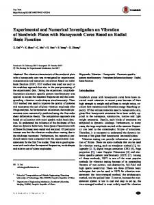
Microphone y
Free stream
NACA0012 c = 100 mm
x
Cylinder R = 10 mm
Figure 1: The sketch of the experiment set-up.
3. Numerical Method Verification 3.1. Numerical Verification. Jacob’s experimental rod-airfoil model was used to validate the proposed numerical method [19]. The experimental set-up and the coordinates are shown in Figure 1. The reference configuration is a symmetric NACA-0012 airfoil (chord: 𝑐 = 0.1 m; thickness: 𝑒 = 0.12 m) located at one-chord distance after the cylinder (𝑑 = 0.1 m), both extending by 𝐿 = 0.3 m in the spanwise direction. The acoustic far field receiver is at 1.85 m from airfoil center. The incoming velocity is 72 m/s and the Reynolds number of the cylinder is 48000. The Reynolds number of airfoil is 480000 with a 0∘ attack angle. The experiment was conducted in the large anechoic room of the ECL (10 m × 8 m × 8 m). The air was supplied by a high-speed subsonic anechoic wind tunnel at Mach numbers ranging up to 0.34. In order to reduce the number of flow meshes, the span of the numerical model is set as 0.05 m which is smaller than the experiment model (𝐿 = 0.3 m). The simulation domain was 𝑋 (−0.3 m, 0.3 m), 𝑌 (−0.2 m, 0.2 m), and 𝑍 (−0.05 m, 0 m). After the grid convergence check, the multiblock structure meshes with 3 million computational grids were used for the RANS/NALS simulation. The first interior point was located at 𝑦+ ≤ 1 from the airfoil surface, yielding a sufficient resolution of the viscous sublayer. In the RANS simulation, the cubic 𝑘-𝜀 turbulence model was used. NLAS provided a more sophisticated subgrid treatment that allowed the extraction of acoustic sources from the temporal variation within the modeled subgrid structures. In this paper, the subgrid was 𝑥 (−0.15 m, 0.15 m), 𝑦 (−0.1 m, 0.1 m), and 𝑧 (−0.05 m, 0 m) with the resolution ratio 0.002. The subgrid located in the noise area is showed in Figure 2. 3.2. The Flow Field. The RANS computations have been conducted with the cubic 𝑘-epsilon turbulence model to generate the unsteady flows. The income velocity is 72 m/s and the open boundary of the experiment is set as the outlet boundary. The unsteady flow information is very important for the turbulence reconstruction procedure. So the very small numerical time step is selected as 0.00001 s. Figure 3 shows the average velocity (𝑈/𝑈0) at 𝑥/𝑐 = 0.25 in 𝑦/𝑐 direction predicted by numerical and experimental methods. The main average velocity predicted by our RANS calculations agrees well with the experimental results especially where the 𝑦/𝑐 is larger than 0.27. Figure 4 shows the lift coefficients of the cylinder and the airfoil. It is interesting that the lift coefficient of the airfoil with a cylinder is different from the
4
Mathematical Problems in Engineering −1.5
Computational gird
0.2
−1 Subgrid −0.5
CL
y (m)
0.1
0
0
0.5 −0.1
−0.2 −0.2
1
−0.1
0
0.1
0.2
1.5 0.002
0.3
x (m)
0.006 Airfoil Cylinder
Figure 2: The computational gird and the subgrid.
0.01
0.014
0.018
0.022
(s)
Figure 4: The lift coefficient of the cylinder and the airfoil. 1.2 0.02
0.01
0.8
y (m)
U/U0
1
0.6
0.4
0
0.1
0.2
RANS Experiment Jacob’s URANS
0.3
0.4
0.5
0
0.6
y/c
Figure 3: The average velocity on the 𝑥/𝑐 = 0.25.
single airfoil without cylinder. The lift of the airfoil in the rodairfoil model presents a sinusoidal oscillation mode, in which its frequency is equal to that of the cylinder. The numerical time step is Δ𝑡 = 0.00001 s so that the oscillating period is 7.1Δ𝑡. It indicates that the Strouhal number of the unsteady flow is 0.1956, which is very similar to that of the Karman vortex street flow. Many researchers had also shown such results, for example, the LES simulation [23]. It indicated again that the RANS simulation has the good accuracy which can be used for acoustic prediction in next step. Generally speaking, for a single airfoil there is a vortex behind the airfoil which is the main aeroacoustic source and produces most components of the noise. But when there is a strong unsteady vortex in front of the airfoil as in Figure 5, the significant aeroacoustic noise would be generated from the front vortex, not the downstream vortex of the airfoil as in Figure 6, because the vortices behind the cylinder
generate the pressure fluctuations on the surface of the airfoil, which becomes the main aeroacoustic source in the rodairfoil model. Particularly when the large vortex behind the cylinder (Figure 5) meets the airfoil, the large upstream vortex would break into small vortices such as in Figure 7 which is the instantaneous flow velocity contour and Figure 8 which is the transient vorticity contour. The two pictures demonstrate how the vortices behind the cylinder interact with the airfoil. It can be seen that the vortices in the opposite direction alternately interact with the airfoil and the strength of the vortices is becoming weaker and weaker with the increase of the downstream distance from the cylinder. At the same time, the broken vortex phenomenon induces the fluctuating pressures on the airfoil surface [24].
Figure 9: The acoustic pressure in time domain. −0.06
0
0.06
0.12
x (m)
Figure 7: The velocity contours.
Above all, in the unsteady flow, due to the interaction between the upstream vortex and the airfoil, the wing leading edge becomes the main noise source in the rod-airfoil model as Jacob’s experiment [19] and other numerical simulation results [24]. 3.3. Acoustic Result. In last section, we qualitatively analyzed the noise sources of the rod-airfoil model. Next we will further compare the numerical simulation far field acoustic results with the experiment data [19]. The far field acoustic receiver in numerical and experimental model is at the 1.85 m from the airfoil center. The advanced time is very important to the acoustic prediction [25], and here the dual-time iteration method is used where the Δ𝑡 = 0.00002 s. Figure 9 presents the acoustics pressure predicted by RANS/NLAS solver in time domain. Figure 10 shows the frequency spectrum of the acoustics pressure levels predicted by our
numerical results and Jacob’s experiment. The numerical results are according to the experiment in high frequency ranging from 85 Hz to 3000 Hz. The predicted peak noise with SPL 91 dB is at 1354 Hz. The amplitude and the frequency both agree well with the experiment results. It indicates that the vortex-structure interaction induced noise of the rodairfoil model can be well predicted by the RANS/NLAS method. In next sections, the validated numerical method will be used to investigate the mechanism of the vortexstructure interaction induced noise for different kinds of rodairfoil model.
4. The Effects of Different Rod Shapes on the Airfoil Noise 4.1. Numerical Models. In the previous study, the RANS/ NLAS method with SPL correction is verified by comparing with the cylinder rod-airfoil experiment test. In this section we will change the shape of the rods to further investigate the mechanism of the vortex-structure interaction induced noise for different rod-airfoil configuration models which
6
Mathematical Problems in Engineering 100 90
0.1
80 0.05
60
y (m)
SPL (dB)
70
50
−0.05
40 30 20
0
−0.1 103 Frequency (Hz)
104 −0.15
Experiment RANS/NLAS
−0.15
−0.1
−0.05
0 x (m)
0.05
0.1
0 x (m)
0.05
0.1
Figure 10: The frequency spectrum of acoustic pressure. 0.1
4.2. The Influence of the Square Rod on the Airfoil Noise 4.2.1. The Flow Field. The lift coefficients of the square rod and the airfoil are shown in Figure 12. They have the same oscillation period. However the amplitude of the oscillation is not stable which is different from the circular rod-airfoil case in Figure 4, especially for the airfoil. We can speculate that the phenomenon is caused by unsteady turbulence flow generated by the square rod which may have significant influence on the fluctuations pressure of the downstream airfoil.
0.05
y (m)
produce different upstream turbulence. The upstream rods include the square column and diamond column with the same characteristic length 𝐷 0.015 m. The chord and span of the airfoil are 15 mm and 400 mm, respectively. The reference configuration is the symmetric NACA 0012 airfoil (chord 𝑐 = 0.15 m, thickness 𝑒 = 0.018 m) located downstream of the rod. In order to decrease the computation cost, the spanwise airfoil in the numerical simulation is reduced to 0.05 m which is smaller than the experiment model’s 0.4 m. The numerical grids after grid convergence for the square rod-airfoil model (1.9 million) and the diamond rod-airfoil model (2.2 million) are as shown in Figure 11. The first interior point is located at 𝑦+ ≤ 1 from the airfoil surface. The numerical status is the same as the experimental test status carried out in CARDC’s 0.55 m ∗ 0.4 m aeroacoustic wind tunnel, with the experiment with the upstream velocity 60 m/s, Ma = 0.176, Re = 90000, 𝑇 = 298.5 K, and 𝑃 = 101325 Pa. The distance between the rod and the airfoil is 150 mm. The acoustic far field receiver is at 0.75 m from the airfoil center. The computation domain for RANS was 𝑋 (−0.35 m, 0.45 m), 𝑌 (−0.3 m, 0.3 m), and 𝑍 (0 m, 0.05 m) and the NLAS subgrid domain is 𝑥 (−0.15 m, 0.15 m), 𝑦 (−0.1 m, 0.1 m), and 𝑧 (0 m, 0.05 m). The sound source resolution is selected as 0.002.
0
−0.05
−0.1
−0.15
−0.15
−0.1
−0.05
Figure 11: The zoomed computation meshes on the 𝑥-𝑦 plane.
The vortex structure behind the square rod in different time steps is shown in Figure 13. There are two vortices existing in downstream behind the square rod. It clearly indicates that the big vortex and the small vortex occur alternatively, which are also becoming the Karman vortex street. However, as shown in the red circles in Figure 13, this is always accompanied with a very small vortex when the large vortex separated from the square rod. The alternative unsteady vortices are obviously different from the circular rod where there is only one large vortex shown in Figure 5. Two-dimensional vorticity contour is more convenient to observe the vortex-structure interaction phenomena directly. Figure 14 shows the vorticity contours in two typical time steps for the cross section at 𝑧 = 0.025. We can see how the vortices were generated, developed, broken, and became of different sizes. Compared with the cylinder rodairfoil model as shown in Figure 8, the irregular positive and negative vortices with larger size behind the square rod alternatively interfere with the downstream wake flow. The
Mathematical Problems in Engineering
7
4 0.02
CL
2
0
Y
0
−2 −0.02 −4 0.02
0.04
0.06
0.08
0.1
0.12
−0.16
t (s)
−0.14
−0.12
−0.1
−0.08
−0.1
−0.08
X
Airfoil Square
4
0.02
2
CL
Y
0
0 −0.02 −2
−4
−0.16
0.04
0.045
0.05 t (s)
0.055
0.06
Airfoil Square
−0.14
−0.12 X
Figure 13: The stream line behind the square rod in different time (up: 𝑡 + 𝑇/4; down: 𝑡 + 𝑇/2).
Figure 12: The lift coefficient of the square rod and the airfoil.
interference effects of the alternative vortices decrease with the increase of the distance along the flow direction. However the interference domain is much bigger than the cylinder model which can reach the rear of the airfoil and the strength of interference is stronger too. The instantaneous 𝑄-vortex isosurfaces of the square rod are also given in Figure 15 which also obviously shows the generation and shedding of the big vortex and small vortex behind the square rod. The interaction of the irregular vortex-shedding with the airfoil significantly changed the fluctuating pressures of the airfoil surface. The oscillation frequency and the amplitude of the lift coefficient are also dependent on the vortex movement. There is obvious connection between the vortex-shedding phase variation and lift amplitude modulation as shown by former research (Phillips, 1956) [7].
4.2.2. Acoustic Results. Figure 16 gives the vortex structure behind the airfoil. We can find that there are two vortices with nearly the same micron size, which are much smaller than those with the size of ten centimeters behind the square rod. It indicates that the unsteady turbulence flow behind the square rod would still be the main aeroacoustic acoustic source as the cylinder rod-airfoil model. Figure 17 is the acoustic pressure distribution identified by the acoustic beam-forming camera. It clearly indicated that the significant acoustic sources are located at the leading edge of the airfoil and also the airfoil surface induced by the fluctuation pressures produced by the upstream turbulence flow. The acoustic far field receiver is located at 0.75 m from the central of the airfoil. The acoustics pressure in time domain was shown in Figure 18. Figure 19 gives the frequency spectrum of the sound pressure levels predicted by the numerical method and experimental test. The max level (SPL = 115 dB) of the experiment appeared at 536 Hz and
the max level (SPL = 111 dB) of the numerical simulation appeared at 509 Hz. The numerical peak frequency and the peak SPL value are a little smaller than the experiment. The sound levels are in agreement with the experiment in low frequency domain and a little larger in high frequency domain. However, generally speaking the trend of the SPL predicted by RANS/NALS agreed well with the experiment data. 4.3. The Influence of the Diamond Rod on the Airfoil Noise 4.3.1. The Flow Field. The stream line behind the diamond rod is given in Figure 20. The details of the vortex-shedding in time domain can be obviously observed. The vortices behind the diamond rod are generated at the same position on the both sides of the diamond rod. The large and small vortices shed alternatively, which is obviously different from
the cylinder rod and square rod. Figure 21 shows the twodimensional vorticity contours at the cross section 𝑧 = 0.025. The density, interference domain, and the strength of the vortices are all bigger than those of the cylinder. The aerodynamic noise level is also expected to be larger than the cylinder rod-airfoil model according to the connections between the vortex and sound radiation [7, 24]. 4.3.2. Acoustic Results. Figure 22 presents the frequency spectrum of the sound pressure level. The peak value of the experimental SPL is 111 dB which appears at 657 Hz and the numerical peak SPL is 109 dB which appears at 680 Hz. In general the tendency of the SPL predicted by the numerical method agrees well with the experiment data. The numerical simulation SPL result is bigger than the experiment data in low frequency domain. However it is in accordance with the experiment data in the middle and high frequency domain
Mathematical Problems in Engineering
9
Figure 15: The instantaneous 𝑄-vortex isosurfaces of the square column.
0.0006
y (m)
0.0003
0
−0.0003
−0.0006 0.1495
0.15
0.1505
0.151
x (m)
Figure 16: The stream line behind the airfoil.
213 100 mm/div
Press. (dB) 114. 113.
100
112. 0
111. 110.
−100
109. 108.
−213 −284
−100
0
100 mm/div
284
107.
Figure 17: The acoustic sources identified by acoustic beam-forming camera.
10
Mathematical Problems in Engineering −0.5
0.03
−1
0.02
−1.5 0.01 y (m)
(Pa)
−2 −2.5
0
−0.01 −3 −0.02
−3.5 −4
0.02
0.04
0.06
0.08
0.1
−0.03 −0.16
0.12
−0.15
−0.14
−0.13 −0.12 x (m)
−0.11
−0.1
−0.15
−0.14
−0.13 −0.12 x (m)
−0.11
−0.1
(s) 0.03
Figure 18: The acoustics pressure in time domain.
0.02 120
y (m)
0.01
SPL (dB)
100
0 −0.01
80
−0.02 60 −0.03 −0.16 40
Figure 20: The stream line behind the diamond column (up: 𝑡+𝑇/4; down: 𝑡 + 𝑇/2). 20
102
103 Frequency (Hz)
104
Experiment RANS/NLAS
Figure 19: The frequency spectrum of the acoustics pressure.
which is the most important to the aerodynamic noise reduction. Figure 23 gives the sound pressure levels of different rod-airfoil configuration models. From both the numerical and experiment results it seems that the noise generated by the square rod-airfoil model is bigger than that of the diamond rod-airfoil model. The frequency of the separation vortices behind the square rod is bigger than those behind the diamond rod, so that the unsteady interference of the square rod is also stronger than the diamond rod. Actually the maximum amplitude of the lift coefficient of the airfoil in square rod-airfoil model is 4 and that of the diamond rodairfoil model is only 2. That is why the noise generated by
the square rod-airfoil model is larger than the diamond rodairfoil model which is the same as the former analysis [7]. The vortex behind the diamond rod is more regular and weaker than the vortex behind the square rod, while it is stronger than that of the cylinder rod, so that in the three rod-airfoil configuration models, the aerodynamic noise of the square rod is the biggest and the noise of the cylinder rod is the smallest. The numerical and experiment results indicate that the vortex-structure interaction plays a very significant role in the flow noise radiation.
5. Conclusions The rod-airfoil configurations are good benchmarks for investigation of vortex-structure interaction induced flow noise. The RANS/NLAS with SPL corrections can give the statistics information of the main flow, the instantaneous vortex structure, and also the acoustic field. It provides a cheap numerical prediction tool with good accuracy and efficiency for the vortex-structure interaction induced noise
reduction. In the low frequency domain the noise predicted by the RANS/NLAS method is a little larger than the experiment data; however the numerical results agree well with experiment results in the middle and high frequency domain. Fortunately, for the wing noise, the characters in the middle frequency domain (e.g., 400–2500 Hz) are usually the most important component for noise reduction. The experiment and numerical results both indicate that the vortex-shedding and broken behavior produced the main acoustic sources for the rod-airfoil model. The vortices behind the square rod are irregular and much more complicated than the diamond rod and the cylinder rod. Compared with the diamond and cylinder rod, the strength of the vortices generated by the square rod is much stronger, which led to the largest flow noise level. With the increase of
Figure 23: The comparison of the frequency spectrum of SPL.
the strength of the upstream vortex, the main acoustic source will extend from the leading edge to trailing edge. An aircraft consists of many components so that there are always vortex-structure interaction phenomena when an aircraft takes off and lands on the ground. Although the noise is also related to the time derivative of the lift and drag components, which are induced by the spanwise vorticity component, the vortex-structure interaction has significant effects on the noise generation and should be paid much more attention in aerodynamic noise reduction. Maybe we could find some vortex-structure interaction noise control method
12 for a realistic landing gear in the significantly higher Reynolds number case, if we could reveal the complex sound radiation mechanism. For the tight connection between the vortex induced unsteady pressure and the noise radiation, maybe an alternative noise control approach should be proposed in the future, for instance, based on the Cp not on the instantaneous lift.
Mathematical Problems in Engineering
[12]
[13]
Conflicts of Interest The authors declare that there are no conflicts of interest regarding the publication of this paper.
[14]
[15]
Acknowledgments This work was partially supported by the National Natural Science Foundation of China (nos. 11672225, 11511130053, and 11272005), the Shaanxi Province Natural Science Foundation (no. 2016JM1007), and the Funds for the Central Universities (2014XJJ0126).
[16]
[17]
References [1] X. Hao, “The progress of civil aircraft high-lift noise research,” in Civil Aircraft Design and Research, vol. 3, pp. 1–7, 2012, http://en.cnki.com.cn/Journal en/C-C031-MYFJ-2012-02.htm. [2] Y. Wang, C. Song, and G. Xu, “Research on effects of flight parameters on helicopter noise in taking off and landing,” Acta AerodynamicaSinica, vol. 3, pp. 321–327, 2010. [3] F. de la Puente, L. Sanders, and F. Vuillot, “On LAGOON nose landing gear CFD/CAA computation over unstructured mesh using a ZDES approach,” in Proceedings of the 20th AIAA/CEAS Aeroacoustics Conference 2014, USA, June 2014. [4] Y. Detandt, “Aeroacoustics research in Europe: The CEAS-ASC report on 2014 highlights,” Journal of Sound and Vibration, vol. 357, pp. 107–127, 2015. [5] W. Dobrzynski, “Almost 40 years of airframe noise research: What did we achieve?” Journal of Aircraft, vol. 47, no. 2, pp. 353– 367, 2010. [6] D. P. Lockard, “A comparison of Ffowcs Williams-Hawkings solvers for airframe noise applications,” in Proceedings of the 8th AIAA/CEAS Aeroacoustics Conference and Exhibit, 2002, Breckenridge, Colorado, USA, June 2002. [7] J. Boudet, D. Casalino, M. Jacob, and P. Ferrand, “Prediction of Broadband Noise: Airfoil in the Wake of a Rod,” in Proceedings of the 42nd AIAA Aerospace Sciences Meeting and Exhibit, Reno, Nevada, 2004. [8] X. Huang, X. Chen, Z. Ma, and X. Zhang, “Efficient computation of spinning modal radiation through an engine bypass duct,” AIAA Journal, vol. 46, no. 6, pp. 1413–1423, 2008. [9] D. Casalino, A. F. P. Ribeiro, E. Fares, and S. N¨olting, “LatticeBoltzmann aeroacoustic analysis of the LAGOON landing-gear configuration,” AIAA Journal, vol. 52, no. 6, pp. 1232–1248, 2014. [10] F. D. da Silva, C. J. Deschamps, A. R. da Silva, and L. G. C. Sim˜oes, “Assessment of jet-plate interaction noise using the lattice Boltzmann method,” in Proceedings of the 21st AIAA/CEAS Aeroacoustics Conference, 2015, June 2015. [11] F. Mathey, “Computation of Trailing-Edge Noise Using a Zonal RANS-LES Approach and Acoustic Analogy,” in Proceedings
[18]
[19]
[20]
[21]
[22]
[23]
[24]
[25]
of the 12th AIAA/CEAS Aeroacoustics Conference (27th AIAA Aeroacoustics Conference), Cambridge, Massachusetts, 2006. R. Ewert, “Broadband slat noise prediction based on CAA and stochastic sound sources from a fast random particle-mesh (RPM) method,” Computers & Fluids. An International Journal, vol. 37, no. 4, pp. 369–387, 2008. J. E. Rosenbaum and E. Boeker, “Enhanced propagation of aviation noise in complex environments: A hybrid approach,” International Journal of Aeroacoustics, vol. 13, no. 5-6, pp. 463– 476, 2014. M. J. Lighthill, “On Sound Generated Aerodynamically. I. General Theory,” in Proceedings of the Royal Society A Mathematical Physical & Engineering Sciences, 1951. C. Kato, Y. Yamade, H. Wang, and M. Miyazawa, “Numerical prediction of sound generated from flows with a low Mach number,” Computers & Fluids, vol. 1, pp. 53–68, 2007. M. Barone, “A computational study of the aerodynamics and aeroacoustics of a flatback airfoil using hybrid RANS-LES,” in Proceedings of the 47th AIAA Aerospace Sciences Meeting, Orlando, Florida, USA, 2009. P. J. Morris, L. N. Long, A. Bangalore, and Q. Wang, “A parallel three-dimensional computational aeroacoustics method using nonlinear disturbance equations,” Journal of Computational Physics, vol. 133, no. 1, pp. 56–74, 1997. P. Batten, E. Ribaldone, M. Casella, and S. Chakravarthy, “Towards a generalized non-linear acoustics solver,” in Proceedings of the 10th AIAA/CEAS Aeroacoustics Conference, Manchester, UK, 2004. M. C. Jacob, J. Boudet, D. Casalino, and M. Michard, “A rod-airfoil experiment as a benchmark for broadband noise modeling,” Theoretical and Computational Fluid Dynamics, vol. 19, no. 3, pp. 171–196, 2005. M. Caraeni, Y. Dai, and D. Caraeni, “Acoustic Investigation of Rod Airfoil Configuration with DES and FWH,” in Proceedings of the 37th AIAA Fluid Dynamics Conference and Exhibit, Miami, Florida, 2007. A. Smirnov, S. Shi, and I. Celik, “Random flow generation technique for large eddy simulations and particle-dynamics modeling,” Journal of Fluids Engineering, vol. 123, no. 2, pp. 359– 371, 2001. C. Kato, A. Iida, Y. Takano, H. Fujita, and M. Ikegawa, “Numerical prediction of aerodynamic noise radiated from low Mach number turbulent wake,” in Proceedings of the 31st Aerospace Sciences Meeting and Exhibit, Reno, Nev, USA, 1993. J. Boudet, D. Casalino, M. Jacob, and P. Ferrand, “Prediction of Sound Radiated by a Rod Using Large Eddy Simulation,” in Proceedings of the 9th AIAA/CEAS Aeroacoustics Conference and Exhibit, Hilton Head, South Carolina, 2003. J. Berland, P. Lafon, F. Crouzet, F. Daude, and C. Bailly, “A parametric study of the noise radiated by the flow around multiple bodies: direct noise computation of the influence of the separating distance in rod-airfoil flow configurations,” in Proceedings of the 17th AIAA/CEAS Aeroacoustics Conference (32nd AIAA Aeroacoustics Conference), Portland, Oregon, 2011. D. Casalino, “An advanced time approach for acoustic analogy predictions,” Journal of Sound and Vibration, vol. 261, no. 4, pp. 583–612, 2003.
Advances in
Operations Research Hindawi Publishing Corporation http://www.hindawi.com