Numerical simulation of fluid-structure interactions with stabilized finite ...

EPJ Web of Conferences 114, 0 2 118 (2016 ) DOI: 10.1051/epjconf/ 2016 11 4 0 211 8  C Owned by the authors, published by EDP Sciences, 2016

Numerical simulation of fluid-structure interactions with stabilized finite element method Petr Sv´aˇcek Czech Technical University in Prague, Faculty of Mechanical Engineering, Dep. of Technical Mathematics, Karlovo n´am. 13, Praha 2, Czech Republic

Abstract. This paper is interested to the interactions of the incompressible flow with a flexibly supported airfoil. The bending and the torsion modes are considered. The problem is mathematically described. The numerical method is based on the finite element method. A combination of the streamline-upwind/Petrov-Galerkin and pressure stabilizing/Petrov-Galerkin method is used for the stabilization of the finite element method. The numerical results for a three-dimensional problem of flow over an airfoil are shown.

1 Introduction There are various technical or scientific applications, where an interaction of flowing fluids and vibrating structures can play an important role, see, e.g. the monographs [1], [2]. The mathematical simulation of fluid and structure interaction is a challenging problem, it requires to consider the viscous, usually turbulent flow, changes of the flow domain in time, nonlinear behaviour of the elastic structure. Moreover, the coupled system for the fluid flow and for the oscillating structure needs to solved simultaneously. The changes of the fluid domain cannot be neglected and the methods with moving meshes must be employed, see e.g. ([3], [4]) . In this paper the numerical analysis of an interaction of the incompressible viscous flow with a vibrating airfoil is considered. The numerical analysis of 2D interactions of the incompressible flow with an airfoil was published in [5], [6]. The method allowing the solution of large amplitude flow-induced vibrations of an airfoil with 3 degrees of freedom (3DOF) was developed and tested in [7]. The approximation of the Navier-Stokes equations in the case of 3D flow problem is much more complicated, see also [8], [9]. The incompressibility can be treated by using the pressure projection methods originated by Patankar, see [10], or Chorin’s artificial compressibility method [11]. The other possibility is to use coupled solution for both pressure-velocity unknownstogether with a multilevel method. For the case of high Reynolds numbers anisotropically refined meshes need to be used in order to capture correctly the boundary layers, wakes, etc. In this paper the attention to the problem of mutual interaction of the airflow with a solid. The motion of the solid is described with the aid of two degrees of freedom (2DOF) (the bending and the torsion modes), which is equivalent to previous two-dimensional (2D) numerical results published, e.g., in [5]. The numerical method based on the fully stabilized finite element method is described.

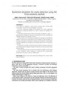
ΓS ΓWt

ΓI

ΓWt

ΓO y x

Γ

S

x z

Fig. 1. The sketch of the computational domain Ωt shown in xy and xz planes. The mutually disjoint parts of its boundary ∂Ωt are shown.

The combination of the streamline–upwind and the pressure-stabilizing Petrov–Galerkin (SUPG/PSPG) and the grad–div stabilization is used. Numerical results are shown.

2 Mathematical model Flow model. In order to practically treat the motion of the fluid computational domain Ωt , the Arbitrary Lagrangian-Eulerian (ALE) method is used, see [12]. The ALE mapping A = A(ξ, t) = At (ξ) defined for all t ∈ (0, T ) and ξ ∈ Ω0ref = Ω0 is assumed to be diffeomorphism of Ω0 onto Ωt at any t ∈ (0, T ). The domain velocity wg (x, t) is then defined by wg (x, t) = ∂A ∂t (ξ, t), where x = A(ξ, t), x ∈ Ωt , ξ ∈ Ω0 . The time derivative with respect to the reference configuration Ω0ref is called the ALE derivative, denoted by DA /Dt and satisfies (see [5], [12]) ∂f DA f (x, t) = (x, t) + wg (x, t) · ∇f (x, t). Dt ∂t

(1)

The incompressible viscous flow in the computational domain Ωt ⊂ R3 is governed by the Navier-

This is an Open Access article distributed under the terms of the Creative Commons Attribution License 4.0, which permits    distribution, and reproduction in any medium, provided the original work is properly cited.

EPJ Web of Conferences

3 Numerical approximation

Stokes equations written in the ALE form DA u + ((u − wg ) · ∇)u = ∇ · σ Dt ∇ · u = 0,

(2)

where u = u(x, t) denotes the velocity vector, u = (u1 , u2 , u3 ), σ denotes the Cauchy stress tensor σ = −pI + ν(∇u + ∇T u), with components σij given by   ∂ui ∂uj , + σij = −pδij + ν ∂xj ∂xi where p = p(x, t) denotes the kinematic pressure and ν is the constant kinematic viscosity (i.e. the viscosity divided by the constant fluid density ρ), t denotes time and δij is the Kronecker’s delta. System of equations (2) is equipped with the initial u(x, 0) = u0 (x)

x ∈ Ω,

(3)

and with boundary conditions a) u = b) u = c) σ · n = d) u · n =

uD on ΓI , 0 on ΓW t , 0 on ΓO , 0, on ΓS ,

(4)

where n denotes the unit outward normal vector to the Lipschitz continuous boundary ∂Ω. The boundary condition (4c) is a modification of the so-called ’donothing’ boundary condition, cf. [13]. Structure motion. The flow motion results in the aerodynamic forces acting on the flexibly supported airfoil, which can be vertically displaced by h (downwards positive) and rotated by the angle α (clockwise positive). In this case the airfoil motion is described with the aid of (nonlinear) motion equations ¨ + Sα cos αα ¨ + kh h = −L(t), mh ¨ + Iα α Sα cos αh ¨ + kα α = M (t).

(5)

where m is the mass of the airfoil, Sα is the static moment around the elastic axis (EA), and Iα is the inertia moment around EA. The parameters kh and kα denote the stiffness coefficients. On the right-hand side the aerodynamical lift force L(t) and aerodynamical torsional moment M (t) are involved, which satisfy  ρσ2j nj dS, (6) L=−  M=

In this section the time discretization of the flow problem is introduced, linearized and the resulting problem is spatially approximated by the finite element method based on continuous piecewise linear (or trilinear) functions is used for approximation of both the velocity and the pressure. The application of the finite element method for the incompressible Navier-Stokes equations needs to overcome two difficulties. First, the velocity-pressure finite element pair needs to be properly chosen in order to guarantee the stability of the scheme, see, e.g., [14], or the PSPG can be used to overcome the instability, see [15]. The second source of the instability is the dominating convection flows. In this case the SUPG method is applied, cf. [16], [17], [18]. 3.1 Time discretization The time interval [0, T ] is divided with a constant time step Δt > 0, i.e. we denote tk = kΔt. Further, we ˙ n) approximate u(tn ), p(tn ), α(tn ), h(tn ), α(t ˙ n ), h(t n n n n n ˙n n and wg (tn ) by u , p , α , h , α˙ , h and wg , respectively. Here, the attention is paid only to the discretization on a fixed time level tn+1 . The ALE derivative in (2) is then approximated by second order backward difference formula (BDF2), i.e. ˜n + u ˜ n−1 3un+1 − 4u DA u  ≈ , (7)  Dlt t=tn+1 2Δt ˜ i (x) = ui (A(ti , ξ)) with x = A(tn+1 , ξ) is the where u transformation of the velocity from the domain Ωti on the domain Ωtn+1 . The convective term is linearized by   ˜n − u ˜ n−1 − wg n+1 ) · ∇un+1 , ≈ (2u ((u − wg ) · ∇)u tn+1

(8) ˜n − u ˜ n−1 − wg n+1 . where we shall write wn = 2u The system of equations (5) is transformed to the first order system and discretized in time using the BDF2, i.e. the following approximations for h˙ and α˙ are used 3αn+1 − 4αn + αn , 2Δt n+1 − 4hn + hn ˙ n+1 ) ≈ 3h , h(t 2Δt

α(t ˙ n+1 ) ≈

and similarly also for the first derivatives 3α˙ n+1 − 4α˙ n + α˙ n , 2Δt ˙ n+1 − 4h˙ n + h˙ n ¨ n+1 ) ≈ 3h . h(t 2Δt

α ¨ (tn+1 ) ≈

ΓW t

ε3ij ri ρσjk nk dS, ΓW t

where ε3ij is the Levi-Civita symbol and ri = xi −xEA i and xEA is the position of the EA at the time instant t.

Further, the aerodynamical lift force and the aerodynamical moment in equations (5) are extrapolated from the previous time levels, i.e. the approximations Ln , M n , Ln−1 , M n−1 are assumed to be computed using (6) and the values of un , pn , un−1 , pn−1 . Then we

02118-p.2

EFM 2015

extrapolate in (5) the aerodynamical lift force and the aerodynamical moment by L(tn+1 ) ≈ 2Ln − Ln−1 ,

M (tn+1 ) ≈ 2M n − M n−1 .

3.2 Spatial approximation Now, the system of equation (2) is time discretized and linearized with the aid of (7) and (8), respectively. Then, the equations are formulated weakly and the solution is sought on the couple of finite element spaces Wh ⊂ H 1 (Ω n+1 ) and Qh ⊂ L2 (Ω n+1 ) for the approximation of the velocity components and pressure. The domain Ω is assumed to be a polyhedral domain and the finite element spaces are defined using an admissible triangulation Th of the domain Ω, cf. [19], such  that Ω = K∈Th K, Th is formed by a finite number of closed hexahedral, tetrahedral, pyramidal or prism elements. Further, on each of reference elements K the local set of shape functions is denoted by PK . For the reference hexahedral element the tri-linear functions are used whereas for the reference tetrahedral element the space PK contains linear functions on K. The consistent definition of PK on the pyramidal or the prism elements can be found in [20]. The finite element spaces are then defined by     3 Qh = ϕ ∈ C(Ω) : ϕ ∈ PK , ∀K ∈ Th , Wh = [Qh ] K

 Xh = ϕ ∈ Wh : ϕ = 0 on ΓI ∪ΓW t , ϕ·n = 0 on ΓS . 

In order to introduce the stabilized weak formulation we start with the definition of the Galerkin terms for any U = (u, p) ∈ Wh × Qh , V = (ϕ, q) ∈ Xh × Qh by 3 (u, ϕ)Ω + (νS(u), S(ϕ))Ω 2Δt n + (w · ∇u, ϕ)Ω − (p, ∇ · ϕ)Ω + (∇ · u, q)Ω , 1 ˜ n−1 , ϕ)Ω , ˜n − u f (u, ϕ) = (4u 2Δt a(U, V ) =

where by (·, ·)Ω the scalar product in L2 (Ω) or L2 (Ω) is denoted. Further, the SUPG/PSPG and div-div stabilization terms are used defined by L(U, V ) =



δK

K∈Th



Fig. 2. The computational domain and the mesh detail around the airfoil shown in the xy-plane.

3u − σ(u) + (wn · ∇)u, (wn · ∇)ϕ + ∇q 2Δt  n   ˜ n−1 ˜ −u 4u F (V ) = , (wn · ∇)ϕ + ∇q δK , 2Δt K K∈Th  τK (∇ · u, ∇ · ϕ)K . P(U, V ) =

where the local element Reynolds number is given by

 ,

Reloc =

K

K∈Th

where (·, ·)K denotes the scalar product in L2 (K) or L2 (K). The choice of the parameters δK and τK is carried out according to [18] or [21] on the basis of the local element length hK , i.e.   h2 h2 , δK = K , (9) τK = ν 1 + Reloc + K ν · Δt τK

hK wn K . 2ν

Then the stabilized discrete problem at a time instant t = tn+1 reads: Find U = (u, p) ∈ Wh × Qh , p := pn+1 , u := un+1 , such that u satisfies approximately the conditions (4 a-b) and a(U, V ) + L(U, V ) + P(U, V ) = f (V ) + F(V ), holds for all V = (ϕ, q) ∈ Xh × Qh . The solution of the arising system of linear equations is realized by a preconditioned iterative method based on inexact LU -factorization.

02118-p.3

EPJ Web of Conferences

4 Numerical results The stabilized finite element method was applied for the approximation of flow over NACA 0015 and NACA 0012 airfoils in the experimental channel, see [22] or [23]. The mutual interaction of the flowing air caused lead to the aeroelastic instability of flutter type. We consider the depth of the domain to be 180 mm (zdirection in Figure 1), the height of the domain (ydirection in Figure 1) to be equal to 210 mm which is the height of the experimental channel of the measurement. The artificial length of the computational domain was chosen to be 7 times the chord of the airfoil. The airfoil chord was equal to c = 18 mm. The computations were performed on hexahedral meshes. The air viscosity was considered to be equal to ν = 1.5 × 10−5 m2 / s. The inlet velocity was set equal to U∞ = 8.33 m / s. The Reynolds number based on the airfoil chord is then equatl to Re = 104 . For the numerical simulation two grids were used. First, the coarse grid consisting of approximately 2 × 105 hexahedral elements was used, where the discrete system with approximately 9×105 unknowns was solved using the iterative solver based on the incomplete blockwise LU factorization. Second, the grid with approximately 700000 hexahedral elements was used leading to the system with approximately 2.8×106 unknowns. The iterative solver was successful in both cases, although the numerical solution on the fine grid required much more computer time (as expected). The further improvement, optimization and parallelization of the iterative solver needs to be done. The solution of the 3D problem was compared to the numerical approximation of the flow in 2D domain, where the grid consisting of the approximately 10000 quadrilateral elements was used. For the 2D problem the solution was realized using the direct solver. The fluid 3D domain is shown shown in Figure 2. The same grid (a slice of the 3D grid) was used for the computation of the 2D flow problem. The results in terms of flow velocity field for 2D and the central plane of 3D computations nearby the airfoil surface are shown in Figure 3.

Furthermore, the iterative method for solution of the discrete problem in 3D was succesfully used. The iterative method based on the blockwise incomplete LU factorization was used. The method was found to be efficient, but for large meshes the convergence was slow (as expected). The improvement of the iterative method will be a subject of future work.

Acknowledgment The financial support for the present project was partly provided by the Czech Science Foundation under the Grants No. P101/11/0207 and 13-00522S .

References 1.

2. 3. 4. 5. 6. 7. 8. 9. 10. 11.

5 Conclusion

12.

This paper focused on the problem of numerical approximation of the incompressible flow with a flexibly supported airfoil. A model problem of channel flow around vibrating NACA 0015 airfoil was considered and mathematically described. The numerical method based on the finite element method was succesfully used for the approximation of the flow problem. This numerical method is the extension of the stabilized finite element method applied succesfully for 2D simulations. Here, however the method was tested and verified by application on a channel flow over the NACA 0012 airfoil. The results were compared to 2D resuls. Furthermore, the numerical approximation based on fully stabilized finite element method was presented and the numerical results for a three-dimensional problem of flow over an airfoil were shown.

13. 14. 15. 16. 17. 18. 19.

02118-p.4

E.H. Dowell, R.N. Clark, A modern course in aeroelasticity, Solid mechanics and its applications (Kluwer Academic Publishers, Dordrecht, Boston, 2004), ISBN 1-402-02039-2 E. Naudasher, D. Rockwell, Flow-Induced Vibrations (A.A. Balkema, Rotterdam, 1994) C. Farhat, M. Lesoinne, N. Maman, International Journal for Numerical Methods in Fluids 21, 807 (1995) P. Le Tallec, J. Mouro, Computer Methods in Applied Mechanics and Engineering 190, 3039 (2001) P. Sv´aˇcek, M. Feistauer, J. Hor´ aˇcek, Journal of Fluids and Structures 23, 391 (2007) P. Sv´aˇcek, Mathematics and Computers in Simulation 80, 1713 (2010) M. Feistauer, J. Hor´ aˇcek, M. R˚ uˇziˇcka, P. Sv´aˇcek, Computers & Fluids 49, 110 (2011) P. Sv´aˇcek, P. Louda, K. Kozel, Journal of Computational and Applied Mathematics 270, 451 (2014) V. John, Int. J. Num. Meth. Fluids 40, 775 (2002) S. Patankar, Numerical Heat Transfer and Fluid Flow (McGraw-Hill, New York, 1980) A.J. Chorin, Journal of Computational Physics 2, 12 (1967) F. Nobile, Ph.D. thesis, Ecole Polytechnique Federale de Lausanne (2001) C.H. Bruneau, P. Fabrie, International Journal for Numerical Methods in Fluids 19, 693 (1994) R. Temam, Navier-Stokes equations. Theory and numerical analysis.s (North-Holland, Amsterdam, 1978) T.J.R. Hughes, M. Mallet, A. Mizukami, Comput. Methods Appl. Mech. Eng. 54, 341 (1986) M. Olshanskii, G. Lube, T. Heister, J. Lwe, Computer Methods in Applied Mechanics and Engineering 198, 3975 (2009) G. Lube, G. Rapin, Computer Methods in Applied Mechanics and Engineering 195, 4124 (2006) T. Gelhard, G. Lube, M.A. Olshanskii, J.H. Starcke, Journal of Computational and Applied Mathematics 177, 243 (2005) P.G. Ciarlet, The Finite Element Methods for Elliptic Problems (North-Holland Publishing, 1979)

EFM 2015

20. C. Wieners, Preprint, University of Stuttgart (1997) 21. P. Sv´ aˇcek, M. Feistauer, Application of a Stabilized FEM to Problems of Aeroelasticity, in Numerical Mathematics and Advanced Application (Springer, Berlin, 2004), pp. 796–805, ISBN 3-54021460-7 22. J. Koz´anek, V. Vlˇcek, I. Zolotarev, Journal of Applied Nonlinear Dynamics 3 (2014) 23. J. Koz´anek, V. Vlˇcek, I. Zolotarev, International Journal of Structural Stability and Dynamics 13, 1 (2013)

Fig. 3. The comparison of the flow velocity pattern for 3D (on the left) and 2D (on the right) computations.

Fig. 4. The comparison of the pressure distribution for 3D (on the left) and 2D (on the right) computations.

02118-p.5