X. Y. YOU, Numerical Simulation of Mass Transfer Performance of Sieve …, Chem. Biochem. Eng. Q. 18 (3) 223–233 (2004)
223
Numerical Simulation of Mass Transfer Performance of Sieve Distillation Trays X. Y. You School of Environmental Science and Engineering, Tianjin University, 300072, Tianjin, P.R. China
Original scientific paper Received: December 4, 2003 Accepted: April 13, 2004
A turbulent mixed two-phase flow model is employed to predict the flow on a column distillation tray by considering the resistance and the enhanced turbulence, which are created by the uprising vapor. The tray flow patterns of our numerical model are confirmed satisfactorily by the experimental measurements. The dependence of mass transfer performance of sieve distillation tray on the physical properties of fluid and tray flow patterns is quantitatively analyzed. Furthermore, the ways to improve the efficiency of distillation sieve are discussed. Keywords: Turbulent two-phase flow, mass transfer performance, distillation, CFD
Introduction Distillation is a widely used method to separate liquid mixtures into their components and has been applied in many separation processes such as those in petroleum, petrochemical, chemical and related industries. It shares a large portion of the capital investment, and is the largest consumer of energy in those industries. It is also commonly recognized that distillation is a very important process in today's industry and will continue to be in the future. Even if the distillation is very old in art, its design method is still lacking a sound basis. For example, although it is well known that the liquid flow pattern, or velocity distribution, is a very important factor in distillation tray design, its evaluation has long been relied mainly on designer's experience or experiment, implicitly in the estimation of tray effectiveness. With the rapid development of computational fluid dynamics (CFD), more reliable theoretical approach of such problem is possible. The tray design based on such scientific foundation is obviously superior to that based on experience or rough estimation, especially for the case of scaling up a column to large diameter. The complication of liquid flow pattern on a column tray comes from the fact that, liquid flowing is aerated through a curved convergent-divergent open channel with structural resistance and subject simultaneously to the action of the cross current uprising vapor. Based on two-dimensional flow with some simplifying assumptions, Yoshida1 presented a direct numerical solution for Navier-Stokes equations in stream function form, nevertheless his result has not been confirmed by experi* Corresponding author, email:
[email protected], tel:+86-22-27403561, fax:+86-22-27402555.
ment. Zhang and Yu2, Yu et al.3 and Liu et al.4 formulated a single-fluid (liquid) model and Yuan et al.5 and Yu et al.6 formulated a two-fluid (liquid and vapor) model for describing the flow patterns on tray. In all these studies, the K - e model is employed to close the Reynolds stress. Their predictions of liquid velocity distribution on the tray were satisfactorily confirmed by the experimental results. The two-fluid model gives slightly better results than those of single-fluid model at the expense of much more complicated computation. Krishna et al.7 and Baten and Krishna8 presented a three-dimensional CFD model and computed by using CFX software for simulating flow field on sieve tray. They found strong 3D effects at the inlet and outlet of a tray and insisted that the 3D simulation is required to include the variations of liquid flow pattern in vertical dimension. However, their test column is of very small diameter, i.e. a very short liquid path in combination with a rather large weir height. From our experimental work and three-dimensional calculation by using commercial software, the steady flow pattern on a tray is mainly two-dimensional except in the regions near the inlet and the outlet weirs and in the thin layer close to the tray floor. We expect that these three-dimensional effects on the flow distribution may be diminished, in percentage of total flow, with the increase of column diameter. Thus, we assume that such three-dimensional effects are negligible here and a two-dimensional flow model can be applied to simulate the flow distribution on the tray. Yu et al.3 studied the concentration field on a sieve tray by applying the CFD method to solve the flow and mass transfer equations with the assumption of constant equilibrium ratio of the separated substance in the mixture. They obtained the mass transfer efficiency in terms of effectiveness of the
224
X. Y. YOU, Numerical Simulation of Mass Transfer Performance of Sieve …, Chem. Biochem. Eng. Q. 18 (3) 223–233 (2004)
tray. But their assumption of constant equilibrium ratio would lead to a large deviation in the case of having wide range of tray concentration. Therefore, a variable equilibrium ratio is adopted to recalculate the concentration field on the tray in this study. Furthermore, the dependence of mass transfer efficiency of sieve distillation tray on the physical properties of fluid and tray flow patterns is quantitatively analyzed and the ways to improve the efficiency of sieve distillation are discussed.
Theoretical model In this paper, we present a two-phase flow model consisting of a continuous liquid phase and a vapor phase dispersed in the form of bubbles and/or froth in the (continuous) liquid phase. The basic equations derived by Elghobashi and Abou-Arab9 for laminar two-phase flows are adopted here. The steady volume average mass and momentum equations for liquid phase are (1)
( r1 f 1U jU i ) ; j =-(1- Mf 2 ) p ;i - MEf 2 (U i -V i ) (2) 2 +[ m 1 f 1 (U i ; j + U j ;i )]; j - ( m 1 f 1U l ;l ) ;i + f 1 . 3 The corresponding equations for vapor phase, i.e. carrying bubbles and froth are ( r 2 f 2V i ) ;i = 0,
(3)
( r 2 f 2V jV i ) ; j =-f 2 p ;i + Ef 2 (U i - V i ) 2 +[ m 2 f 2 (V i ; j + V j ;i )]; j - ( m 2 f 2V l ;l ) ;i + f 2 . (4) 3 and the global continuity equation is f 1 + f 2 = 1.
(5)
In equations (1)-(4), the partial derivatives are represented by a subscript consisting a semicolon and an index [e.g., U i ; j = ¶U i ¶x j , U i ; jl = ¶ 2U i ¶x j ¶x l ]. M is the local effectiveness of momentum transfer from the dispersed phase to the continuous phase. M =1 is chosen here by assuming a perfect momentum exchange between the two phases. Assuming that, in the flowing aerated liquid, the velocity of carrying bubbles and froth Vi is equal to that of liquid phase Ui. By adding equations (1) and (3), simplifying the result and applying equation (5), we have ( rU i ) ;i = 0 .
( rU jU i ) ; j =- p ;i + [ m(U i ; j + U
j ;i
)]; j -
2 - ( mU l ;l ) ;i + f . 3
(6)
(7)
where r = r1 f 1 + r 2 f 2 and m = m 1 f 1 + m 2 f 2 are the density and viscosity of mixture. For turbulent flow, the volume fractions f1 and f2 are separated as a mean value and a disturbance f 1 = f 1 + f¢1 , f 2 = f 2 + f¢2 .
Two-phase flow model
( r1 f 1U i ) ;i = 0,
Similarly by adding equations (2) and (4), it results
(8)
The above equations lead to a flow with variable density and viscosity even if the density and viscosity of the two phases are assumed to be constants here. Similarly, we have r = r + r¢, m = m + m¢.
(9)
For turbulent flow with variable density, the density-weighted average, called Favre-average, should be applied to turbulence velocity instead of applying the conventional Reynolds-average, that is ~ (10) U i = U i + U ¢¢i , U i = rU i r. Then the Favre-average equations for mass and momentum are ~ (11) ( rU i ) ;i = 0, ~ ~ ( rU jU i ) ; j =- p ;i +
(12)
é ~ 2 ~ ù ~ +ê m(U i ; j + U j ;i ) - mU l ;l ú - ( rU ¢¢iU ¢¢j ) ; j + f , û ë 3 ;j
~ where U i denotes the Favre-average velocity. rU ¢¢iU ¢¢j is the Reynolds stress and modeled by the eddy viscosity assumption as é ~ 2 ~ ~ ù 2 rU ¢¢iU ¢¢=m tê(U i ; j +U j ;i )- d ijU l ;l ú+ rKd ij . j û 3 ë 3 Here dij is the Kronecker delta and K is turbulent kinetic energy. In equation (12), the contributions from the viscosity disturbance are neglected and the Favre-average velocity is assumed to be equal to the Reynolds-average velocity, see Gatski10 for details. The K - e turbulence model is applied here and the equations for turbulent kinetic energy and turbulent dissipation rate are éæ ù mt ö ~ ÷ ( rU j K ) ; j =êç çm+ ÷K ; j ú + P - re , (13) sk ø û ëè ;j
X. Y. YOU, Numerical Simulation of Mass Transfer Performance of Sieve …, Chem. Biochem. Eng. Q. 18 (3) 223–233 (2004)
éæ ù mt ö e e2 ~ ÷ ( rU j e ) ; j =êç çm+ ÷e ; j ú +c1 P-c 2 r , (14) sk ø û K K ëè ;j where mt is turbulent viscosity, P = Pt + Pv is the production rate of turbulent kinetic energy, Pt and Pv are corresponding to the turbulent kinetic energy produced by the horizontal turbulent flow and the uprising vapor, respectively. The Pv will be defined in Section 2.1.3. mt and Pt are expressed as mt = cm r
K2 ~ , Pt =- rU ¢¢iU ¢¢j U i ; j . e
The above cm, c1, c2, sk and se are the K - e turbulence model constants. The flow field is shown in Figure 1. The boundary conditions for the equations (11)–(14) are defined below.
~ ~ U 1; 2 = K ; 2 = e ; 2 = 0 , U 2 = 0 .
225
(17)
The boundary conditions at tray wall are determined by the wall functions, see Liu et al.4 We drop all superscripts of averaged quantities ~ in the present and subsequent sections, i.e. write U i as Ui and r as r for simplification. Phase volume fraction and clear liquid height
The condition of two-phase flow on trays is in one of the following three different regimes: bubble regime, drop (spray) regime and froth regime. In most cases, column trays are operated in froth regime, see Stichlmair and Fair11 for a detailed discussion. By comparing many published correlations for the volume fraction of liquid phase, Stichlmair12 suggested that the volume fraction of liquid phase can be approximated as æ F ö0. 28 ÷ f 1 = 1-ç ç ÷ , è F max ø where F = U g
F max = 2.5 [a 2p s
(18)
r 2 is the vapor load factor and
g ( r1 - r 2 )]0. 25 is the maximum vapor load factor. The equation (18) is valid for F < 3, and all cases calculated here are in this range. The height of clear liquid hl is given by experiments (see Yu et al.3) as h l = 8.04 +3.05 Ls+2.523 h w0. 5-3.612 ´10-3 F 2 . (19) F i g . 1 Flow field on the tray
For the inlet boundary, the inlet liquid velocity distribution is assumed to be uniform. The inlet turbulent kinetic energy and turbulent dissipation rate are described by the following empirical expressions Ls ~ ~ ~ U 1in = , U 2in = 0 , K in = 0.003 U 12in , hl 1. 5 (15) 009 . K in e in = . 003 . ´ 05 . W Here, hl is the clear liquid height. At the outlet boundary, the flow is assumed being fully developed, then ~ (16) U i ;1 = K ;1 = e ;1 = 0 . The flow field is symmetric to the centerline. The boundary conditions at the centerline are
Resisting force exerted by vapor phase
The uprising vapor, which crosses the flowing aerated liquid, or liquid mixture, on a distillation tray, undergoes mutual momentum exchange. Consequently, the uprising vapor exerts a resisting force on the flow and this resisting force is approximated by (see Zhang and Yu2) f =-c f
r 2U g U i hl
,
(20)
where the coefficient cf reflects the imperfect momentum exchange between the uprising vapor and the flowing aerated liquid on the tray. The above expression implies a hypothetical assumption that the vapor phase leaving the flow surface obtains a horizontal velocity component equal to cfUi. It is obvious that cf depends on the height of clear liquid. After many tests, we choose c f =1. 7 h l in all our calculations. For the convenience of statement, we designate afterward the “aerated liquid” as “liquid phase”.
226
X. Y. YOU, Numerical Simulation of Mass Transfer Performance of Sieve …, Chem. Biochem. Eng. Q. 18 (3) 223–233 (2004)
Turbulent energy created by bubbling action
Besides the resisting force exerting on the flow, the uprising vapor offers a direct contribution to the turbulent energy on the liquid phase flow. This fact is obvious because the liquid phase on the tray is fluctuating even if its mean velocity is zero, i.e. no liquid phase flow. The quantity of this extra turbulent energy, Pv, is related to the operating conditions. For simplification, the uprising vapor through a single hole of sieve plate is considered to estimate the turbulent energy from bubbling action. In principle, such a flow consists of three essential periods, i.e. a converging period before the plate, a diverging period after the plate and finally, the period of passing through the flowing layer, as shown in Figure 2.
Dh =
=
p ge - p go g p2
U g2
2 g a h2 a 2p
+
2 U ge - U g2
2g
- hl = (23)
(1- a k a p ) 2 - h l .
Since the pressure head loss hl is consumed to overcome the hydrostatic pressure head, the vapor energy loss per volume, which produces the turbulent kinetic energy, is expressed as Pv =c p
r 2 ( gDh+ghl )U g hl
=
c p r 2U g3 2 a h2 a 2p hl
(1- a h a p ) 2 . (24)
Where cp is a parameter for imperfect energy transfer between the uprising vapor and the flow on a tray. Obviously, it will depend on the inlet velocity and the height of clear liquid. We suggest using the empirical expression c p = 6.63 ´10-9U in2 h w3 .
(25)
Mass transfer model
F i g . 2 Vapor passing a sieve plate hole
The velocity Uge is related to the gas velocity Ugh by the mass conservation, via U ge =
U gh Ah Ae
=
U gh ah
=
Ug
ah a p
,
(21)
where the hole discharge coefficient, ah is 0.611 for the sharp edged holes at high Reynolds number, see Stichlmar and Fair11 for details, ap is the relative free area of the sieve tray. The pressure loss during vapor passing through the flow layer is approximately determined by considering the pressure loss along a pipe with a nozzle inside, see Olson and Shelstad,13 we have p ge - p go = r 2U g (U g - U ge ).
(22)
Then, the pressure head loss for the uprising vapor is
The successful application of the CFD to the prediction of velocity field on a tray may lead to the development of a method to evaluate the corresponding concentration field, from which the estimation of tray effectiveness can be established on a more theoretical and reliable basis. In this study, we suppose the mass transfer between vapor and liquid phases has no influence on the velocity field on the tray. This assumption is reasonable if the rate of mass transfer between the two phases is not very high. The effect of mass transfer on the velocity field will be a subject of another study. In distillation process, counter-diffusion occurs simultaneously. That means the light component diffuses from liquid to vapor phase and, at the same time, the heavy component diffuses from vapor to liquid phase. In the present paper, we only concern one plate (tray) where the mass concentration change is usually very small, possibly from few percents to little over ten percents. In a narrow concentration range, the change of heat of vaporization is relatively small and therefore, in engineering practice, we may assume the amount of counter-diffusion to be approximately equal over a plate (tray). For the computation of whole column, it should be considered the change of the heat of vaporization over the whole mass concentration range. In our model, we consider the composition of vapor phase being identical with that of bubbles or froth. The governing equations for the equal molar transfer in the liquid phase, containing bubbles and froth, are expressed as
X. Y. YOU, Numerical Simulation of Mass Transfer Performance of Sieve …, Chem. Biochem. Eng. Q. 18 (3) 223–233 (2004)
( f 1U j C1 ) ; j - ( D1 f 1C1; j ) ; j +k1 a (C1 -C1i ) = 0 , (26) ( f 2U j C 2 ) ; j - ( D2 f 2C 2; j ) ; j +k 2 a (C 2i -C 2 ) = 0 , (27)
where C 1¢ and C ¢2 are the concentrations of light component at the liquid and bubbles (or froth) respectively. Considering the turbulent effects of the flow field, the following fluctuation equations can be written C i = C i + C 1¢ , C ii = C ii + C ii¢ , k i = k i + k ¢i,
a = a + a¢,
(28) (29)
Substituting the above equations together with equations (8) and (10) into equations (26) and (27) and neglecting the correlation of any two scalar disturbances and the higher order correlation such as r¢C ¢i , k ¢i a¢, aC ¢i , r¢C ¢iU ¢¢j etc., see Abou-Arab,14 as
light component at the interface and can be approximately expressed by Raoult's law as x&1i = g p 0 x& 2i = H x& 2i .
(30)
then the equations (26) and (27) become ( f 1U j C 1 ) ; j - [( D1 + D t ) f 1C 1; j ) ; j + +k1 a(C 1 - C 1i ) = 0 , ( f 2U j C 2 ) ; j - [( D 2 + D t ) f 2C 2; j ) ; j + +k 2 a(C 2i - C 2 ) = 0 ,
(31)
K1 =
where Dt is the phase turbulent diffusion coefficient. As stated in previous section, all superscripts ~ of averaged quantities are dropped, i.e. U i written as Ui and r as r for simplification. Furthermore, by substituting C i = rx& i into equations (31) and (32), we have f 1U j x&1, j - f 1 [( D1 + D t )x&1; j ]; j + + k1 a ( x&1 - x&1i ) = 0 , f 2U j x& 2, j - f 2 [( D 2 + D t )x& 2; j ]; j + + k 2 a ( x& 2i - x& 2 ) = 0 ,
x&1* = H x& 2 , x&1 = H x& *2 .
= K 1 ( x&1 - x&1* ) = K 2 ( x& *2 - x& 2 ).
(37)
Substituting equations (35) and (37) into equations (33)-(34), we have f 1U j x&1, j - f 1 [( D1 + D t )x&1; j ]; j + + K 1 a ( x&1 - Hx& 2 ) = 0 ,
(38)
f 2U j x& 2, j - f 2 [( D 2 + D t )x& 2; j ]; j + æ x&1 ö + K 2 aç - x& 2 ÷= 0 . èH ø
(39)
The boundary condition for equations (38) and (39) is described below. For the inlet boundary, we assume the concentrations of light component in liquid and in carrying bubbles or froth are x&1in and 0, respectively, i.e. (40)
At the outlet boundary, the concentration field of light component is assumed being fully developed, then (41)
x& i ;1 = 0 .
The mass fraction field is symmetrical to the centerline and the boundary condition is (42)
x& i ;2 = 0 .
(33)
On the wall, since it cannot be penetrated by the light component, the boundary condition may be written to be
(34)
¶x& i = 0. ¶r
The mass transfer flux between liquid and gas phases can be expressed as N s = k&1 ( x&1 - x&1i ) = k 2 ( x& 2i - x& 2 ) =
H k1 k 2 k1 k 2 , K2= , Hk1 + k 2 H k1 + k 2
x&1 = x&1in , x& 2 = 0 . (32)
(36)
Then from equations (35) and (36), we have
well as replacing the correlation U ¢¢j C ¢i by U ¢¢j C ¢i =-D t C i ; j .
227
(35)
where Ns is the mass transfer flux between the two phases. x&1i and x& 2i are the molar concentrations of
(43)
Mass transfer coefficients and interfacial area
According to Stichlmar and Fair,11 the mass transfer coefficients in liquid and vapor sides can be estimated by the following equations, applicable to froth and drop regimes k1 =
4f 1 D1U g p hl f 2
, k2 =
4f 1 D 2U g p hl f 2
. (44)
228
X. Y. YOU, Numerical Simulation of Mass Transfer Performance of Sieve …, Chem. Biochem. Eng. Q. 18 (3) 223–233 (2004)
The interfacial area can be expressed, respectively, for bubble regime as follows (F F max > 0.35) 0. 28 é 6g ( r1 - r 2 ) ù0. 5æ F ö ç ÷ a b =ê ÷ . ú ë û ç s è F max ø
(45)
0. 28 ù F2 é æ F ö ç ÷ ê 1 ç ÷ ú. 2sa 2p ê ë è F max ø ú û
(0.55- F F max ) a b + ( F F max - 0.35) a d . (47) (0.55 - 0.35)
Evaluation of mass transfer efficiency
The mass transfer efficiency of a tray is related to the concentration distribution. For the generalization of concentration expression, a dimensionless liquid concentration Xi is introduced and defined as follows Xi =
x& i - x& *i
x& iin - x& *i
.
(48)
In which X i =1 and X i = 0 represent the initial and equilibrium conditions, respectively. Substituting x& *i (see equation (37)) into equation (48), the dimensionless liquid concentration becomes X1 =
x&1 - Hx& 2 . x&1in - Hx& 2
nw
åi=1
X 1i
.
(50)
(46)
For the interfacial area of froth regime (0.35 < F F max > 0.55), Stichlmar and Fair11 suggested to interpolate the interfacial areas of bubble regime and drop regime (equations (45) and (46)). Here we take the weighted average of the interfacial areas of bubble regime and drop regime as that of froth regime, af =
np
åi=1 X 1i
Then the computation of h, the relative tray efficiency of a tray, is possible by the aid of CFD.
and for drop regime (F F max > 0.55) ad =
1 np h= 1 nw
(49)
We now define a new term h, called the relative mass transfer efficiency of a tray or simply the relative tray efficiency, to be the ratio of the average dimensionless liquid concentration on the whole tray to that at the outlet weir. Thus h=1 represents the condition of perfect mixing of liquid phase on the tray. In the case of partial mixing of liquid phase, h is greater than 1. Under the condition of no mixing, i.e. the plug flow, h reaches to maximum value. Obviously, h is a measure of the mixing characteristics on a tray, similar to the conventional expression of enhancement factor, E MV EOG . The value of h can be conveniently computed by the value of X1 at each grid obtained from the numerical computation as follows
Numerical results and discussion The discretization of the mixed turbulent two-phase flow model (equations (11)–(14)) at grids is performed by finite volume method. The discrete control equations are solved by SIMPLEC algorithm, see Doormal and Raithby15 for details. After the velocity field on the tray is obtained, the mass transfer model (equations (38) and (39)) is solved to compute the concentration distribution of light component and the relative tray efficiency h. The K - e turbulence model constants based on the experimental work of Launder16 in a tunnel flow are c1 = 1. 44, c 2 = 1.92, c m = 0.09, s k =1.0, s e =1.3. The numerical results of Yu et al.3 show the above constants should be modified in order to fit the experimental data for sieve trays. After a number of trials, the constants c1 = 1. 48 and c 2 = 1.98 are found to be more sensitive than other constants. For the best fitting, they suggested to use c1 and c 2 for tray velocity simulation. In the present study, constants c1 = 1. 48, c 2 = 1.98, c m = 0.09, s k =1.0, s e =1.3. are adopted in all our calculations. Our numerical simulation is based on two experimental trays. We call the tray, on which Porter et al.17 carried on their experiment, to be Porter tray and the tray, on which Liu18 did his experiment, to be Liu tray. The geometric parameters for Porter tray and Liu tray are D = 2. 44 m , W D = 0.615 and D =1.2 m , W D = 0.645, respectively. In this study, r1 = 1000 kg m -3 , m 1 = 1´10-3 kg m -1 s-1 , r 2 = 1.2 kg m -3 and m 2 = 2 ´10-5 kg m -1 s-1 are adopted as the density and viscosity of the two phases, respectively. According to the rule of similarity, there exists a relationship between the turbulent kinematic viscosity and the turbulent diffusion coefficient. Yu et al.3 show that slightly different ratio of the above two parameters does not change substantially the results of the concentration profile on the tray. Here we take their suggested relationship D t =1.25 m t r for all calculations.
229
X. Y. YOU, Numerical Simulation of Mass Transfer Performance of Sieve …, Chem. Biochem. Eng. Q. 18 (3) 223–233 (2004)
Flow field simulation
Figures 3 shows the comparison of the results of our mixed two-phase flow model with those by experiments. Here the percentage of circulation region T is defined as the ratio of the circulation area to the whole tray area. This parameter is essentially important for sieve tray design. In fact, the T value should be reduced to be as small as possible to achieve the best velocity distribution and the relative tray efficiency.
T a b l e 1 The addopted parameters of diferent computing cases Unit Figure 4
Ls 2 –1
m s
0.02
Figure 5
hw
Ug –1
ap
s –1
H
D1 2 –1
m s
D2 m2 s–1
mm
ms
20
1.5
0.1
0.1
2
10–9
10–6
20
1.5
0.1
0.1
2
10–9
10–6
1.5
0.1
0.1
2
10–9
10–6
0.1
0.1
2
10–9
10–6
0.1
2
10–9
10–6
2
10–9
10–6
10–9
10–6
Figure 6
0.02
Figure 7
0.02
20
Figure 8
0.02
20
1.5
Figure 9
0.02
20
1.5
0.1
Figure 10 0.02
20
1.5
0.1
Nm
0.1
F i g . 3 The percentage of circulation region % vs. liquid flow rate. Porter tray (P): D = 2.44 m, hw = 20 mm, Ug = 1.5 ms–1, Liu tray (L): D = 1.20 m, hw = 50 mm, Ug = 1.0 ms–1
It is found that the T value increases with the increase of input liquid flow rate Ls and the results of our numerical flow model are in a good agreement with the corresponding experiments.
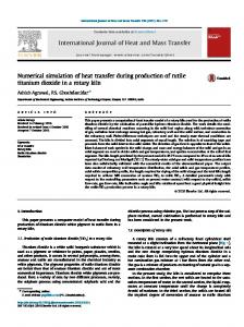
F i g . 4 Contour map of liquid dimensionless concentration on Liu Tray
Relative tray efficiency h estimation
Table 1 shows the adopted parameters of Figures 4–10. Figure 4 is the contour map of dimensionless concentration in liquid X1 on sieve tray. It shows there is a large backward mixing area (vortex) near the tray wall and the X1 value is low at that area. Then the relative tray efficiency h is greatly reduced by the backward mixing effects. The larger the mixing area, the smaller the plate effectiveness is. Figure 5 shows the dependence of h on the input liquid flow rate for Porter tray and Liu tray. For both trays, the h value decreases with the increase of Ls. The reason is that with the increase of Ls the input liquid velocity is increased and results in the increase of the percentage of circulation region. It is noted that the h value of Porter tray is always larger that of Liu tray as seen from Figures 5–10.
F i g . 5 Relative tray efficiency vs. liquid flow rate. Solid line: Porter tray, dashed line: Liu tray
230
X. Y. YOU, Numerical Simulation of Mass Transfer Performance of Sieve …, Chem. Biochem. Eng. Q. 18 (3) 223–233 (2004)
Figure 6 shows the dependence of h on the height of outlet weir hw. As hw increases, the input liquid velocity is decreased for the same input liquid flow rate. Based on the same explanation for Figure 5, the h value is increased with the increase of hw. But this dependence on hw is much weaker than that on Ls. Figure 7 shows that the h value increases with the increase of superficial gas velocity for both trays. With the increase of Ug, the mass transfer coefficients ki and the turbulent kinetic energy Pv produced by the uprising vapor are increased. The increase of Pv will results in the reduction of the backward mixing area. Both reducing the mixing area and increasing the mass transfer coefficients can increase the h value. Figure 8 shows the dependence of h on ap. The value of h decreases fast with the increase of ap when ap < 0.1 for Porter tray and ap < 0.08 for Liu
tray. Then the decrease changes to be slight. The reason for this change may be explained as follows. With the increase of ap, Pv and ad decrease and causes the lowering of h. On the other hand, f1 increases with the increase of ap. This leads to the increase of k1 and k2 and cause the increase of h. These two opposite effects cause the h value decreases slightly with the increase of ap. Figure 9 shows the dependence of h on s. The value of h decreases fast with the increase of s when s < 0.05 for both trays. Then it decreases slightly when s > 0.05. The effects of s on the value h are very complex and have at least three aspects. Firstly, the interfacial area is decreased with the increase of s and this effect causes the decrease of h. Secondly, f1 increases with the increase of s, which leads to the increase of k1 and k2 and cause the increase of h. Thirdly, the increase of s also changes the mixture of vapor and liquid, which may
F i g . 6 Relative tray efficiency vs. outlet weir height. Solid line: Porter tray, dashed line: Liu tray
F i g . 8 Relative tray efficiency vs. plate free area rate. Solid line: Porter tray, dashed line: Liu tray 2
F i g . 7 Relative tray efficiency vs. superficial gas velocity. Solid line: Porter tray, dashed line: Liu tray
F i g . 9 Relative tray efficiency vs. surface tension. Solid line: Porter tray, dashed line: Liu tray
X. Y. YOU, Numerical Simulation of Mass Transfer Performance of Sieve …, Chem. Biochem. Eng. Q. 18 (3) 223–233 (2004)
change the Reynolds number and turbulence intensity of the flow field, and results in the change of velocity field and the h value. The first two effects are local effects that are independent on tray diameter, but the third effect is an effect on the whole tray (flow field), which surely depends on the tray diameter. Figure 10 shows the dependence of h on H. The results indicate that h increases slightly with the increase of H. The constant H shows the interfacial resistance when mass transferring at the interface. The higher value of H means the smaller drive force term of interfacial mass transfer K 1 ( x&1 - Hx& 2 ) in equations (38) and (39) if the two-film model is adopted. For the flow field of the same tray, this is similar to the case of the two phases with less on-tray contact time, such as the plug flow case, where h gets to a larger value. Here we should note that the constant H we put in Raoult’s law is only valid for small concentration range of light component in liquid and vapor over a tray. In case of large concentration range of light component, the constant H is varying due to the change of activity coefficient g with concentration for non-ideal separating system. Fortunately, it is shown that H has only small effects on h. Thus, it is quite safe to say that the deviation introduced by assuming H to be a constant should be negligible.
F i g . 1 0 Relative tray efficiency vs. H. Solid line: Porter tray, dashed line: Liu tray.
Our results also show h value increases fast with the increase of D1. The coefficients of mass transfer K1 and K2 increase when D1 increases and leads to the fast increase of h. On the other hand, the dependence of h on D2 is very weak and h value increases slightly with the increase of D2. It is concluded that D1 has stronger influence on the mass transfer between the liquid and vapor than D2. This conclusion also comes simply by looking at the
231
constants of D1 and D2. Except the effect of H, the mass transfer of interface is always controlled by the smaller molecular diffusion phase until a equilibrium state is reached.
Conclusions It is shown, that the turbulent mixed two-phase flow model presented here can be applied to simulate the gas-liquid flow on the tray instead of using the much more complicated two-fluid model without losing much accuracy. Computations show that the percentage of circulation region on the tray has large effects on the relative tray efficiency, i.e. the performance of mass transfer over a tray. The larger the percentage of circulation region is, the smaller the relative tray efficiency. In order to increase the relative tray efficiency, it is necessary to investigate how to reduce the percentage of circulation region. Numerical results show that the relative tray efficiency can be efficiently increased as a result of improving the flow pattern on a tray. The high relative tray efficiency can be realized by optimized operational and geometric parameters, such as by increasing outlet weir height hw, superficial gas velocity Ug, or by reducing liquid flow rate Ls and plate free area rate ap (ap < 0.1). On the other hand, the relative tray efficiency can also be improved by changing some physical properties of liquid and vapor, such as reducing the surface tension s in the range of s < 0.05. But the constant H, gas diffusion coefficient D2 and surface tension s at s > 0.05 have only small effects on the relative tray efficiency. Results also show that the relative tray efficiency of Porter tray (larger diameter tray) responses more strongly to the above discussed ways of improving tray performance than that of Liu tray (smaller diameter tray). This means the mass transfer performance of a large diameter tray is more sensitive to the parameters studied here. This may be explained as: for most of ways above to improve the performance of trays, the flow pattern on the trays always be affected in a way or another. Comparing to a large diameter tray, the inertia of reducing circulation region on a small diameter tray is large due to its large curvature of tray boundary, numerical results show that the circulation of flow affects the relative tray efficiency strongly. That is why the mass transfer performance of a small diameter tray is less sensitive to the parameters studied here. The distillation process is a very complex system. It is strongly affected by many operational, physical and geometric parameters. To achieve high relative tray efficiency, more study is necessary to
232
X. Y. YOU, Numerical Simulation of Mass Transfer Performance of Sieve …, Chem. Biochem. Eng. Q. 18 (3) 223–233 (2004)
look for the optimal design and operating parameters of a distillation process. Finally, it should be mentioned that the above ways to improve the mass transfer performance of trays only present a general rule for optimizing or designing trays. Which methods are accepted in a real case is dependent on the carefully consideration and the evolution of all-important factors (including economy and manufacture). It should be avoided, that the improvement of one side by neglecting the price to be paid for this, on the other side. ACKNOWLEDGEMENTS The author would like to acknowledge many helpful discussions of Prof. K. T. Yu and Prof. X. G. Yuan of Tianjin University and the support of the Distillation Laboratory of the State Key Associated Laboratories of Chemical Engineering (China) at Tianjin University. I also thank the reviewer for many valuable comments to improve the manuscript. Notation
a – interfacial area per unit volume A – area c1, c2, cm – K - e model constants – momentum transfer parameter cf cp – energy transfer parameter cq – mass transfer parameter – concentration of light component C – tray diameter D Di – phase molecular diffusion Dt – phase turbulent diffusion – interfacial friction coefficient E EMV – Murphree tray effectiveness EOG – Murphree point effectiveness – body and external force. f – vapor load factor F – acceleration due to gravity g – constant put in Raoult's law H – clear liquid height hl hw – outlet weir height – turbulent kinetic energy K Ki – mass transfer coefficient – phase mass transfer coefficient ki Ls – liquid flow rate Ns – mass transfer flux between phases np – grid number on tray nw – grid number at outlet weir – pressure p p0 – saturation vapor pressure – turbulent energy production P
Pv – R – r – T – Ug – Ui, Vi – W – xi – – x& i * – x& i Xi
turbulent energy produced by uprising vapor tray radius radial coordinate percent of circulation region superficial gas velocity phase velocity width of outlet weir Cartesian coordinates molar concentration of light component equilibrium molar concentration
– phase dimensionless concentration
Greek symbols
ah – ap – e – h – m – mi – mt – r – ri – s – sk, se – fi –
area rate free area rate of sieve tray turbulent energy dissipation rate relative tray efficiency mixture viscosity phase viscosity turbulent viscosity mixture density phase density surface tension K - e model constants phase volume fraction
Superscripts
– ´ ~ " i
– – – – –
Reynolds-average value disturbance in Reynolds-average Favre-average value disturbance in Favre-average phase interfacial surface
Subscripts
1 2 ;i b d f h in
– – – – – – – –
liquid phase or light component in liquid phase vapor phase or light component in vapor phase derivative with respect to xi bubble drop froth hole value at inlet weir
References 1. Yoshida, H., Chem. Eng. Comm. 51 (1987) 261. 2. Zhang, M. Q., Yu, K. T., Chinese J. Chem. Eng. 2 (1994) 63. 3. Yu, K. T., Liu, C. J., Yuan, X. G.., 1999 Annual Meeting of American Institute of Chemical Engineers, Dallas.
X. Y. YOU, Numerical Simulation of Mass Transfer Performance of Sieve …, Chem. Biochem. Eng. Q. 18 (3) 223–233 (2004)
4. Liu, C. J., Yuan, X. G., Yu, K. T., Chem. Eng. Sci. 55 (2000) 2287. 5. Yuan, X. G., You, X. Y., Yu, K. T., J. Chem. Ind. Eng. (China) 46 (1995) 511. 6. Yu, K. T., Yuan, X. G., You, X. Y., Liu, C. J., Chem. Eng. Res. Des. 77 (1999) 554. 7. Krishna, R., van Baten, J. M., Ellenberger, J., Higler, A. P., Taylor, R., Chem. Eng. Res. Des., 77 (1999) 639. 8. van Baten, J. M., Krishna, R., Chem. Eng. J. 77 (2000) 143. 9. Elghobashi, S. E., Abou-Arab, T. W., Phys. Fluids 26 (1983) 931. 10. Gatski, T. B., Turbulent flows: model equations and solution methodology, Computational Fluid Mechanics, ed. Peyret, R., Academic press, 1996. 11. Stichlmair, J. G., Fair, J. R., Distillation, Wiley-VCH, 1998.
233
12. Stichlmair, J. G., Grundlagen der Dimensionierung des Gas/Fluessigkeit-Kontakt-apparates Bodenkolonnen Verlag Chemie, Weinheim, New York, 1978. 13. Olson, S. T., Shelstad, K. A., Introduction to fluid flow and the transfer of heat and mass, Prentice-Hall, Inc., 1987. 14. Abou-Arab, T. W., Turbulence model for two-phase flows, Encyclopedia of Fluid Mechanics, Vol. 3, Ed. Cheremisinoff, N. P., Gulf Publishing Company, 1985. 15. van Doormal, J., Raithby, G. D., Numer. Heat Transfer 7 (1984) 147. 16. Launder, B. E., Morse, A., Rodi, W., Spalding, D. B., Proc. of NASA conference on free shear flow, Langley, 1972. 17. Porter, K. E., Yu, K. T., Chambers, S., Zhang, M. Q., Flow patterns and temperature profiles on a 2.44m diameter sieve tray. IChE Symp. Ser., 1992, pp. 128. 18. Liu, C. J., Ph. D. Dissertation, Tianjin university, 1998.