European Congress on Computational Methods in Applied Sciences and Engineering ECCOMAS 2004 P. Neittaanm¨ aki, T. Rossi, S. Korotov, E. O˜ nate, J. P´ eriaux, and D. Kn¨ orzer (eds.) Jyv¨ askyl¨ a, 24–28 July 2004
NUMERICAL SIMULATIONS OF THE WAKE VORTEX NEAR FIELD OF HIGH-LIFT CONFIGURATIONS Eike Stumpf? , Jochen Wild? , Adil A. Dafa’Alla† and Ernst A. Meese‡ ? DLR,
Institute of Aerodynamics and Flow Technology Lilienthalplatz 7, 38108 Braunschweig, Germany e-mail:
[email protected],
[email protected] †
Airbus UK, Dept. Flight Physics P.O. Box 77, Filton, Bristol, BS99 7AR, United Kingdom e-mails:
[email protected] ‡
SINTEF Materials and Chemistry, Dept. Flow Technology Alfred Getz vei 2, 7465 Trondheim, Norway
[email protected]
Key words: wake vortex, C-Wake, high-lift, Euler, jet-vortex interaction Abstract. Euler simulations of the nearfield wake of the DLR-F11 model in take-off configuration and a very large transport model in landing configuration are performed using the DLR TAU code on unstructured grids. The aim of the investigation is firstly to analyse the predictive capability of an Euler code for high-lift configuration vortex wakes and secondly to study configuration effects on the vortex wake nearfield. A grid adaptation strategy and parameter settings for the flow simulation are determined by validation with 5-hole probe measurement results that lead to good agreement between simulation and experiment at a half wing span downstream of the model wing tip. The identical simulation procedure is applied to a very large transport aircraft configuration and the interaction between the outer engine jet and the flap side-edge vortex is investigated.
1
E. Stumpf, J. Wild, A.A. Dafa’Alla and E.A. Meese
1
INTRODUCTION
World airports face a long-term capacity problem due to the air traffic control separation regulations presently in use. These air traffic control separation regulations determine the minimum longitudinal distance between two aircraft on the same flight path dependent on the maximum take-off weights of both aircraft in order to prevent the following aircraft from encountering potentially hazardous wake turbulence. The attempts to alleviate wake vortices in the early seventies lost importance upon proving the system of empirically-found separation standards to be a suitable measure to ensure safe air traffic operations. Meanwhile, due to the increasing number of congested airports and the development of very high capacity transport aircraft, the research efforts on the wake vortex problem have risen again. Present computer technology does not allow Navier-Stokes simulations of vortex wakes of high-lift configurations on a regular basis. Thus, for the investigation of configuration effects on vortex wakes it is reasonable to fall back on the use of Euler codes. Already in the mid eighties Mitcheltree et al. [10] demonstrated that vortex trajectories up to 4 chord length can be simulated in good agreement to measurement results even with coarse grid resolution. Nonetheless to date, still a challenge is a realistic simulation of vortex core growth and development of vorticity distribution based on the Euler equations. Strawn [14] and Lockard & Morris [9] found vortex radii too large by a factor of 2-3 a few chord lengths behind a rectangular wing. Over-prediction of vortex radii by a factor of 1.5 − 2.5 is also shown by Stumpf et al. [15] a half span downstream of the model wing tip of a transport aircraft in high-lift configuration. However, one chord length downstream of the model wing tip vortex radii smaller than measured in the wind tunnel are found. Similar under-predictions were reported by Spall [13]. The reason is that simulations based on the Euler equations require the use of grids with medium resolution in order to introduce through numerical diffusion a realistic level of artificial viscosity. Hence, the grid becomes part of the physical model. The needed grid resolution is not known a priori, but has to be determined by comparison with corresponding measurement results. This can be regarded as a calibration of the numerical grid. Following computations by Stumpf et al. [15, 16] for different aircraft models a similar level of accuracy is achieved in flow solutions if the parameters of mesh generation, mesh adaptation and flow solver are kept identical. Thus, not necessarily for all considered configurations validation experiments are required. The aim of the present paper is to evaluate the predictive capability of the DLR-TAU code for the simulation of complex high lift configuration vortex wakes with a future industrial use in the regular design process in mind. In a first step the simulation procedure, consisting of mesh generation and flow simulation followed by subsequent mesh adaptation steps, is validated with wind tunnel measurement results of the DLR-F11 wide-body model. In a second step the simulation procedure is applied to a very large transport aircraft (VLTA) in landing configuration.
2
E. Stumpf, J. Wild, A.A. Dafa’Alla and E.A. Meese
2
USED FLOW SOLVER: DLR TAU
The DLR-TAU [3] code is a finite volume Euler/Navier-Stokes solver working on unstructured and hybrid grids. Local time-stepping and multigrid for convergence acceleration is included. The inviscid fluxes are calculated by employing a second order central scheme with scalar dissipation [4]. A grid adaptation module enables the primary grid to be adapted to the solution if an enhanced resolution is required in certain regions of the computational domain. As an indicator for the adaptation the total pressure gradient is used. 3
VALIDATION OF SIMULATION PROCEDURE
The simulation procedure is validated against wind tunnel measurements performed within the European research programme C-Wake [1]. 3.1
Validation Test Case
The test case for the vortex wake simulation of a complex geometry is the DLR-F11 model in take-off configuration. That is a wide-body airliner model with a half span of b/2 = 1.4m, sharp edged wing and flap tips and blunt trailing edges. Fig. 1 shows the F11 model used for the simulation. In take-off configuration the deflection of the flaps is δF lap = 22◦ and the deflection of the slats δSlat = 20◦ . The horizontal tail plane (HTP) is set to δHT P = −15◦ . Within the framework of the European project C-Wake the vortex wake of the F11 has been experimentally investigated in the DNW-NWB low speed wind tunnel in Braunschweig. The F11 half model was mounted on a 6-component balance. Additionally to the balance data, pressure measurements in 11 rows of pressure tabs on the wing, slat and flap were performed and the flow downstream was examined in three planes perpendicular to the wind tunnel axis using a rake of 18 probes. Each probe was of the 5-hole type. The rake had been carefully aligned and calibrated before the test. Flow condition of the test case was M∞ = 0.2, ambient temperature and pressure. The angle of attack of α = 13.1◦ leads to a lift coefficient of cL = 1.76. 3.2
Numerical Set-up
For the vortex wake nearfield simulation the flow solver TAU based on the Euler equations is used. Since Euler calculations overpredict lift considerably the angle of attack and the HTP deflection angle must be adjusted in order to achieve the correct HTP force contribution and the measured lift coefficient of cL = 1.76. Based on previous experience [16] for the initial grid the needed α-reduction was estimated to be ∆α = −1◦ and the HTP deflection was decreased by one degree to δHT P = −14◦ . An alternative approach of accounting for the viscous effects by adjusting the flap angle to allow for further decambering of the wing could also be used [2]. For the nearfield TAU simulation the central difference scheme [4] with standard dissi3
E. Stumpf, J. Wild, A.A. Dafa’Alla and E.A. Meese
pation coefficient settings k (2) = 1/2 and k (4) = 1/64 is employed. The initial grid is generated with the commercial tool ICEM Tetra. 3.3
Mesh Adaptation
TAU includes a mesh adaptation module which is used to successively increase the mesh resolution of the distinct vortices and vorticity layers, in total 10 adaptation steps were performed. The convergence history of the simulation is shown in Fig. 2. The measure of the convergence of the flow solution is the l2 -norm of the density residual. Within the first 150 iteration steps the density residual decreases by four orders of magnitude, before, due to the first adaptation step, the residual increases abruptly by 1.5 orders of magnitude. This cycle recurs in a similar way for all 10 adaptation steps. In Fig. 2, also the convergence of the lift coefficient and the stepwise function of the number of numerical domain points are shown. The initial grid has 1.1 × 10⁶ points, the 10 times adapted grid 6.4 × 10⁶ points. In order to analyse the vortex core resolution in Fig. 3 the number of grid points per vortex core radius rc is plotted for different adaptation levels exemplary for the wing tip vortex. In its early development stage the wing tip vortex is not circular. The vortex core boundary is assumed to coincide with the maximum circumferential velocity in radial direction. The number of points within this bounded area is determined and the number of points per radius is calculated for a circular substitute vortex with equidistant point distribution. Fig. 3 shows that the initial grid resolves the wing tip vortex radius up to x/b = 0.5 constantly with 2 grid points. With each mesh refinement the resulting vortex core radii decrease. However, as seen in Fig. 3, the TAU adaptation module is capable to increase the number of points per radius in the wing tip vortex core, after 10 adaptation steps the average resolution amounts to 40 points per radius. 3.4
Spanwise Lift Distribution / HTP Pressure Distribution
If a configuration does not include a HTP it is shown e.g. in [15, 16] that a simple angle of attack adjustment can lead to good agreement with measurement results. With HTP the angle of attack reduction and HTP deflection adjustment has to be determined iteratively. In the present F11 case with HTP four iteration steps were needed to obtain the appropriate α-reduction from αExp = 13.1◦ to αSim = 12.55◦ and HTP adjustment from δHT P,Exp = −15◦ to δHT P,Sim = −13.8◦ . The simulation result of the spanwise lift distribution on the 7× adapted mesh is shown in Fig. 4. The graph represents the sum of the contributions of the flaps, main wing and slats, the symbols are the measured values in the DNW-NWB. Fig. 5 shows a comparison of the calculated and measured HTP pressure distribution in the available spanwise cut y/bHT P = 0.462. Both the calculated spanwise lift distribution and the HTP pressure distribution show good agreement with the experimental results.
4
E. Stumpf, J. Wild, A.A. Dafa’Alla and E.A. Meese
3.5
Vortex Wake Nearfield
A comparison of the wind tunnel measurements with numerical results obtained on a 7× and 10× adapted mesh at x/bq= 0.5 is shown in Fig. 6-8. Contour variable is normalized cross-flow velocity vc /u∞ = (v 2 + w2 )/u∞ in 8 levels 0.05 < vc /u∞ < 0.5. The grey border in Fig. 6 represents the limits of the measured field. The topology of the simulated vortex wake shows both with medium and fine mesh resolution a good agreement with the measurement. The positions of the vortex centers and the rotation of the wing tip vortex around the flap tip vortex are almost identical. In Fig. 9 the vertical velocity component w/u∞ is shown in a cut through the flap and wing tip vortices. The position of the cutting line is depicted in Fig. 8. From Fig. 9 it becomes evident that each adaptation steps leads to higher maximum vertical velocity and smaller vortex core radii. The ratio of vortex core radii of the simulation rSim and the experiment rExp of the wing tip vortex on the initial grid is rSim /rExp = 3.7 and decreases in subsequent adaptation levels to rSim /rExp = 1.92 for the 7× and rSim /rExp = 1.72 for the 10× adapted mesh. The maximum simulated vertical velocity matches the experimental results best on the 7× adapted grid. The ratio of maximum vertical velocities max(wSim )/max(wExp ) increases from a value of 47% on the initial grid to 63% on the 5× and 104% on the 7× adapted mesh. On the 10× adapted mesh the maximum vertical velocity is with a ratio of 130% significantly over-predicted. Subsequent adaptations steps would worsen the simulation result. The fact of obtaining simultaneously an overprediction of vortex core radius and peak circumferential velocity may be in parts explained with dispersive effects stemming from the numerical method used, i.e. the flow field is spread without energy dissipation due to the grid cell faces being oblique to the flow. The energy dissipation is mainly due to the the artificial dissipation included in the numerical scheme to ensure stability. Simulations on grids with grid lines closely aligned to the axial flow direction show much less dispersive numerical effects as demonstrated by CFD norway in [16]. The vorticity distribution in the same cut is shown in Fig. 10. The simulated distribution shows outside of the vortex center regions a good agreement with the measurement. However, the peak vorticity on the vortex axes is simulated too low in all cases. The maximum vorticity levels are obtained on the 10× adapted grid with 55% of the experimental value in the wing tip vortex and 58% in the flap tip vortex. Fig. 11 shows that the circumferential velocity distribution vθ = f (r) of the wing tip vortex in the simulation on the 7× adapted mesh can be approximated nearly perfectly with the Lamb-Oseen vortex model whereas a Lamb-Oseen fit of the experimental result fails. A Lamb-Oseen vortex is an exact solution of the incompressible Navier-Stokes equations in the case of Beltrami flow in which a vortex grows solely by viscous diffusion and an asymptotic solution for 2D-vortical structures in high Reynolds number flows on a large time scale [12]. On a short time scale, as considered in the present investigation, the model is a good representation of real vortices only at very low Reynolds numbers
5
E. Stumpf, J. Wild, A.A. Dafa’Alla and E.A. Meese
(Re ≤ 105 ), as shown e.g. in [8]. For Reynolds numbers of the order of Re ≥ 106 the Lamb-Oseen model gives a poor fit, see also Jacquin et al. [5]. Thus in turn it can be concluded that in the present simulations the effective vicosity due to numerical diffusion is very high (and respectively the Reynolds number calculated with the effective viscosity very low) despite an average resolution of the wing tip vortex radius with 30 points. The relative kinetic energy, analysed for the plane at x/b = 0.5 both with the cross-flow velocity Ekin,2D = 0.5(v 2 + w2 ) and all velocity components Ekin,3D = 0.5(u2 + v 2 + w2 ), is shown in Fig. 12. The kinetic energy is evaluated only within the area in which measurement data is available and the energy is normalized with the experimental result. The axial velocity component is dominant: In the experiment the share of kinetic energy resulting from the cross-flow velocity Ekin,2D,Exp amounts merely to 2.27% of Ekin,3D,Exp . A comparison of the simulation with the experimental result in Fig. 12 shows that on the initial grid a value of Ekin,3D,Sim /Ekin,3D,Exp = 92.5% is obtained, further mesh adaptation leads to 99.4% for the 7× and 99.8% for the 10× adapted mesh. While for conservation of axial momentum coarse grids are sufficient, fine grids are needed for the realistic simulation of rotational kinetic energy Ekin,2D . On the 5× adapted mesh Ekin,2D,Sim is equal to 34% Ekin,2D,Exp , the 7× adapted mesh gives 105% Ekin,2D,Exp and the 10× adapted mesh 107.4% Ekin,2D,Exp . Thus, circulation, vortex positions, circumferential velocity and relative kinetic energy agree well with the experiment for the adaptation level 7, but the radius is predicted too large by a factor of 2. This would be impossible if the velocity distributions in the experiment would be similar to Lamb-Oseen profiles. However, realistic vortices show a different distribution leading to less circulation within the vortex core area and less kinetic energy compared to a Lamb-Oseen vortex with equal core radius and total circulation. The presented flow simulation and mesh adaptation strategy leads to good results with the DLR Tau code. This investigation does not allow to derive general rules since the local mesh resolution and the impact of discretization of equations and time integration cannot be universally quantified. However, a similar Euler approach was also successfully adopted by Dafa’Alla [2] on a typical civil aircraft high lift model which lend more confidence to the validity of the approach 4
APPLICATION OF SIMULATION PROCEDURE
The afore presented simulation procedure is applied to a VLTA model in landing configuration, as shown in Fig. 13. 4.1
Application Test Case
The VLTA model geometry includes flaps, flap track fairings, slats, aileron, nacelles and pylons. An enlarged view of the slat cut-outs in the region of the engine pylons reveals the complexity of the geometry, see Fig. 14. In landing configuration the flaps are deflected with δF lap = 32◦ the slats δSlat = 26.5◦ resp. 30◦ and the aileron with δAileron = 10◦ .
6
E. Stumpf, J. Wild, A.A. Dafa’Alla and E.A. Meese
The lift coefficient is cL = 1.85. Flight speed is M a = 0.2 at ambient temperature and pressure. The VLTA model is equipped with turbine powered engine simulators (TPS). The development of jet plumes is driven by three effects: The jet plumes adjust to the ambient pressure, they are deformed by the interaction with dicrete vortices of the wake and air is entrained into the jet plumes. The last effect is a viscous phenomenon which requires, similar to vicous vortex cores, the use of grids with medium resolution in order to introduce through numerical diffusion a realistic level of artificial viscosity. Since no validation data is available qualitative reasoning is adopted. Two TPS power settings are investigated: idle power setting with fan rev of R = 11000rpm and go around setting with R = 54000rpm. The jet temperature is equal to ambient temperature. 4.2
Numerical Set-up
The numerical set-up is identical to the one used for the validation test case. The basic mesh, generated with ICEM Tetra, contains 1 × 10⁶ points, after 7 adaptations steps the number of points for the final mesh increased to 6 × 10⁶ points. As adaptation indicator the gradient of total pressure loss is employed, areas with negative total pressure loss, i.e. the engine jets are excluded. However, in any case the grid refinement outside the engine jet boundaries leads, due to regularity constraints of the mesh, also to a refinement within the jet plume areas. 4.3
Vortex Wake Nearfield
The simulation results in a plane perpendicular to the onflow direction at a downstream distance of x/b = 0.5 are shown in Fig. 15. On the left side the simulation result with the go-around power setting is shown while the idle power setting is shown on the right side. The contour variable in Fig. 15 is normalized vorticity. The vortex topology is very similar for both power settings. In each case three strong vortices can be distinguished: above the main wing the wing tip vortex is found, which is rotated by 1/8 revolution around the strong flap vortex. Inboard, near the fuselage a counter-rotating vortex stemming from the inner side-edge of the inner flap is seen. However, Euler computations neither predict the fuselage boundary layer nor the turbulent wake flow behind the fuselage. It can be expected that in the real case the inner vortices interact with the fuselage boundary layer and dissolve quickly due to the turbulent fuselage wake. Between the fuselage and the outboard flap vortex remnants of the outboard vortex of the inner engine nacelle can be identified by means of strong streamline curvature. This vortex is co-rotating with the wing tip vortex. The counter-rotating inner nacelle vortex does not survive the roll-up process. At the outer nacelle in the same way no counter-rotating inner vortex is found. The co-rotating outer nacelle vortex is a part of the vorticity area
7
E. Stumpf, J. Wild, A.A. Dafa’Alla and E.A. Meese
below the outboard flap vortex. An evaluation of the vortex position shows insignificant differences in vortex position between the result with idle and go-around power setting, see Table 1. Basically the vortex ∆y/b ∆z/b
Wing Outer Flap Inner Flap 0.048% -0.034% -0.16% 0.33% 0.35% 0.35%
Table 1: Differences in Vortex Position positions are independent of the investigated power setting. A quantitative comparison of the radial circulation distribution of the three distinct vortices is shown in Fig. 16. Again, no impact of the power setting is observed. In Fig. 17 the distribution of total pressure in the extracted plane at x/b = 0.5 is displayed. Negative total pressure loss marks the engine jets. The high introduced axial momentum in the case of the go-around power setting leads to larger engine jet cross-areas. However, the over-all topology of the engine jets is similar for both power settings. In both cases the jet of the outer engine is entrained into the outer flap vortex in a way that strongly resembles Fig. 1 in Paoli et al. [11]. In the present simulations the wrapping process is slightly more progressed in the low power setting case. An enlarged view of the outer engine jet with go-around power setting at x/b = 0.5 is shown in Fig. 18. The area with negative total pressure loss, i.e. the engine jet, is displayed in black. It is interesting to note that the wrapping process of the engine jet follows partly the corresponding Kaden roll-up spiral [7] as depicted in Fig. 18. From theoretical work and numerical simulations by Jacquin & Pantano [6] and Paoli et al. [11] it is known that during the entrainment phase the jet spirals in a helix-shape with decreasing radius in the outer potential vortex region towards the vortex axis. But, the solid body rotation of the vortex core prevents the jet to intrude into the core region such that it is accumulated in a ring-like structure around the vortex core. In good agreement, in the present Euler simulations the engine jet remains outside the vortex core region, as demonstrated in Fig. 18. The inserted viewgraph in the upper left corner shows the cross-flow velocity of the outer flap vortex in the cut A–B, as depicted in Fig. 18. The peak cross-flow velocities mark the vortex diameter which is confined to the eye of the engine jet spiral, indicated by the dashed lines. 5
CONCLUSIONS
Euler simulations of the nearfield wake of the DLR-F11 model in take-off configuration and a VLTA model in landing configuration have been performed using the DLR TAU code on unstructured grids. The aim of the investigation was firstly to analyse the predictive capability of an Euler code for high-lift configuration vortex wakes and secondly to study configuration effects on the vortex wake nearfield. Some general conclusions can 8
E. Stumpf, J. Wild, A.A. Dafa’Alla and E.A. Meese
be drawn from the investigation: • The neglect of viscosity is justifiable since the adjustment of the lift coefficient by a reduction of the angle of attack and of the deflection angle of the HTP has been proven to be an appropriate measure to simulate a realistic vortex formation in the nearfield. A grid adaptation strategy and parameter settings for the flow simulation have been determined by validation with 5-hole probe measurement results that lead to good agreement between simulation and experiment concerning spanwise lift distributions, wake topology and vortex positions at a downstream distance of x/b = 0.5. • An average vortex core radius resolution with 30 points (7× adapted grid) gives an exact agreement of the simulated maximum tangential velocity with the experimental result, but the core radius is overpredicted by a factor of rSim /rExp = 1.92 and the peak vorticity is significantly underpredicted. With an average vortex radius resolution of 40 points (10× adapted grid) the maximum tangential velocity is simulated too large, whereas still vortex core radius is over- and peak vorticity underpredicted due to dispersive effects caused by the numerical scheme. • In this context also the steady flow assumption should be challenged. The good convergence proves steady flow in the simulation result. However, from PIV measurements it is known that the DLR-F11 vortices oscillate. Thus, time averaged 5-hole probe measurements do not necessarily result in physical vortices which limits their validity for code validation. • The flow simulation based on the Euler equations leads to vortices which match LambOseen model vortices whereas the measured velocity profiles significantly differ from corresponding Lamb-Oseen profiles. That is to say, in the simulations the effective viscosity due to numerical diffusion is dominant. Viscous diffusion rules the vortex development despite the fine grid resolution and masks vortex stretching and tilting effects. • In the case of a close coupling between engine jet and side-edge vortex the Euler simulations show that the jet is entrained into the vortex but remains outside the vortex core boundaries. • The side-edge vortex dominates the jet plume development, in opposite direction no impact is found. Vortex positions and radial circulation distributions at a downstream distance of x/b = 0.5 are basically independent of engine jet axial momentum, respectively engine power setting. • The successful simulation of the wake flows in this study, as well as others, shows that the Euler approach can be an effective affordable approach to provide initialisation nearfield data to be used in conjunction with any mid-to-far-field computations with any other advanced CFD method. • A possible future improvement to the pure Euler approach, aiming to maintain reasonable computational costs, is to include modelling of the viscous and turbulent effects localized around the vortex cores. This would reduce the grid dependency of the model and allow grid convergence of the solution upon refinement. Also, hexagonal cells aligned with the flow direction should be considered to reduce dispersive effects. 9
E. Stumpf, J. Wild, A.A. Dafa’Alla and E.A. Meese
REFERENCES [1] E. Coustols, E. Stumpf, L. Jacquin, F. Moens, H. Vollmers and T. Gerz. Minimised Wake: a Collaborative Research Programme on Aircraft Wake Vortices. AIAA 2003938, 41st Aerosp.Sci.Meet. & Exhibit, Reno, 2003 [2] A. Dafa’Alla. Computations of the wake vortices behind a civil aircraft high lift model. AIAA 2004-1235, 42nd Aerosp.Sci.Meet. & Exhibit, Reno, 2004. [3] M. Galle. Ein Verfahren zur numerischen Simulation kompressibler, reibungsbehafteter Str¨omungen auf hybriden Netzen. Dissertation, DLR-FB 99-04, 1999. [4] A. Jameson, W. Schmidt and E. Turkel. Numerical solutions of the Euler equations by finite volume methods using Runge-Kutta time stepping schemes. AIAA 81-1259, Palo Alto, 1981. [5] L. Jacquin, D. Fabre, P. Geffroy and E. Coustols. The properties of a transport aircraft wake in the extended near field - An experimental study. AIAA 2001-1038, 39th Aerosp.Sci.Meet. & Exhibit, Reno, 2001 [6] L. Jacquin and C. Pantano. On the persistence of trailing vortices. J. Fluid Mech, 471, 159–168, 2002. [7] H. Kaden. Aufwicklung einer unstabilen Unstetigkeitsfl¨ache. Ing. Archiv, II, 140–168, 1931. [8] T. Leweke and C.H.K. Williamson. Cooperative elliptic instability of a vortex pair. J. Fluid Mech., Vol. 360, 85–119, 1998 [9] D.P. Lockard and P.J. Morris. Wing-Tip Vortex Calculations Using a High-Accuracy Scheme. J.aircraft, 35, 728–738, 1998. [10] R.A. Mitcheltree, R.J. Margason and H.A. Hassan. Euler Equation Analysis on the Initial Roll-Up of Aircraft Wakes. J.aircraft, 23, 650–655, 1986. [11] R. Paoli, F. Laporte, B. Cuenot and T. Poinsot. Dynamics and mixing in jet/vortex interactions. Phys.Fluids., 15, 1843–1860, 2003. [12] L. Rossi and J. Graham-Eagle. On the Existence of Two-Dimensional, Localized, Rotating Self-Similar Vortical Structures. SIAM J. Appl. Math., 62, 2114–2128, 2002. [13] R.E. Spall. Numerical Study of a Wing-Tip Vortex Using the Euler Equations. J. Aircraft, 38, 22–27, 2001. [14] R.C. Strawn. Wing Tip Vortex Calculations with an Unstructured Adaptive-Grid Euler Solver. in proc. 47th Annual Forum American Helicopter Soc., Phoenix, 1991. 10
E. Stumpf, J. Wild, A.A. Dafa’Alla and E.A. Meese
[15] E. Stumpf, R. Rudnik and A. Ronzheimer. Euler computation of the nearfield wake vortex of an aircraft in take-off configuration. Aerosp.Sci. & Techn., 4, 535–543, 2000. [16] E. Stumpf, M. Hepperle, D. Darracq, E.A. Meese, G. Elphick and S. Galpin. Benchmark Test for Euler Calculations of a High Lift Configuration Vortex Wake. AIAA 2002-0554, 42nd Aerosp.Sci.Meet. & Exhibit, Reno, 2002. FIGURES
Figure 1: DLR-F11 model.
residual ||dρ/dt|| 10
7
-1
densityresidual 10
points per radius
cL points x106 cL
50
points 6
10x adapt.
2
-2
40
5
7x adapt.
4
30
10-3 1 10
3 20
5x adapt.
10
3x adapt. initial grid
2
-4
1 10-5 500
1000
0
0
0
Figure 2: Convergence History
0
0.1
0.2
0.3
0.4
0.5
x/b
iterations
Figure 3: Points per radius of wing tip vortex
11
E. Stumpf, J. Wild, A.A. Dafa’Alla and E.A. Meese
Figure 4: F11 Spanwise Lift Distribution
Figure 5: F11 cP -distribution on HTP
Figure 6: F11 Cross-flow velocity measurement, x/b = 0.5, 8 levels 0.05 < vc /u∞ < 0.5
12
E. Stumpf, J. Wild, A.A. Dafa’Alla and E.A. Meese
Figure 7: F11 Cross-flow velocity simulation on 7× adapted mesh, x/b = 0.5, 8 levels 0.05 < vc /u∞ < 0.5
Figure 8: F11 Cross-flow velocity simulation on 10× adapted mesh, x/b = 0.5, 8 levels 0.05 < vc /u∞ < 0.5
13
E. Stumpf, J. Wild, A.A. Dafa’Alla and E.A. Meese
w u∞
Initial grid 5x adapt. 7x adapt. 10x adapt. Experiment
0.5 0.4 0.3
ω b/2 u∞
Wing Vortex
Flap Vortex
100
Wing Vortex
Experiment 75
0.2 0.1
Flap Vortex
0
50
7x 5x
Initial 5x
-0.1
25
Initial grid
-0.2
7x 10x
-0.3 0.3
0.35
0.4
0.45
0 0.5
0.3
y/b
0.35
0.4
0.45
0.5
y/b
Figure 9: F11 Vertical velocity distribution
vθ max(vθ)
10x
1
Figure 10: F11 Vorticity distribution
Simulation
0.8
0.6
Experiment
0.4
0.2
Lamb-Oseen Fit 0
0
0.005
0.01
0.015
r/b
Figure 11: F11 Circumferential velocity of wing tip vortex: experiment versus simulation (7× adapted mesh)
14
Figure 12: F11 Kinetic energy
E. Stumpf, J. Wild, A.A. Dafa’Alla and E.A. Meese
Figure 13: VLTA model.
Figure 14: Details of VLTA geometry
15
E. Stumpf, J. Wild, A.A. Dafa’Alla and E.A. Meese
Figure 15: VLTA Vorticity distribution at x/b = 0.5, 61 levels |min| = max
Γ Γ0
1
Outboard Flap Vortex
0.75 0.5
11000 rpm 54000 rpm
0.25 0
Γ Γ0
0
1
0.03
r/b
0.06
Wing Tip Vortex & Inboard Flap Vortex
0.75 0.5
11000 rpm 54000 rpm
0.25 0
0
0.01
r/b
0.02
Figure 16: VLTA Radial circulation distribution at x/b = 0.5
16
E. Stumpf, J. Wild, A.A. Dafa’Alla and E.A. Meese
Figure 17: VLTA Total pressure loss distribution at x/b = 0.5, 71 levels |min| = max
vc u∞
z (b/2)
A-B
0.2
0.05
A
B 0
0.1 0.675
0.7
0.725
-0.05
-0.1
-0.15
-0.2 0.6
0.7
0.8
y/ (b/2)
Figure 18: VLTA Engine jet spiral at x/b = 0.5, rev = 54000rpm, 2 levels: white → 1 − ∆p/p∞ > 0, black → 1 − ∆p/p∞ < 0
17