Numerical Solutions to Poisson Equations Using the Finite-Difference Method James R. Nagel Terahertz Device Corporation Salt Lake City, Utah 84124 USA E-mail:
[email protected]
Abstract
The Poisson equation is an elliptic partial differential equation that frequently emerges when modeling electromagnetic systems. However, like many other partial differential equations, exact solutions are difficult to obtain for complex geometries. This motivates the use of numerical methods in order to provide accurate results for real-world systems. One very simple algorithm is the Finite-Difference Method ( F DM), which works by replacing the continuous derivative operators with approximate finite differences. Although the Finite- Difference Method is one of the oldest methods ever devised, comprehensive information is difficult to find compiled in a single reference. This paper therefore provides a tutorial-level derivation of the Finite- Difference Method from the Poisson equation, with special attention given to practical applications such as multiple dielectrics, conductive materials, and magnetostatics. Keywords: Partial differential equations; numerical simulation; finite difference methods; electrostatics; magnetostatics
r, Equation (1) simplifies into the familiar, classical fonn of Poisson's equation, given by
1 . Introduction
W
hen studying the behaviors of complex physical sys tems, we frequently desire knowledge about the electric and magnetic field distributions produced by unique spatial arrangements of charge and current. Such information can be especially useful for designers who intend to optimize the per formance of sophisticated electrical devices. For many situa tions, this usually requires the solution of an advanced partial differential equation under specified boundary conditions. Unfortunately, exact analytical solutions are difficult to obtain for most geometries of practical interest. We must therefore resort to approximation methods, if we ever expect to obtain any useful information about them at all.
(2) with/being called the/arcing/unction. For the case of /
=
0,
Equation (2) then takes on another familiar form: (3) which is the well-known Laplace equation.
the unknown function for which we wish to solve under specific boundary conditions. For the special case when u lover all
Like most partial differential equations, closed-form solu tions to the Poisson and Laplace equations only exist for a small handful of simplistic models. Many computational algo rithms exist for generating approximate numerical solutions, but one of the oldest and simplest of these is called the Finite Difference Method (FDM) [1-5]. As the name implies, the Finite-Difference Method works by replacing the continuous derivative operators of Poisson's equation with finite-differ ence approximations, and then numerically solving the resul tant system. The accuracy of the Finite-Difference Method is therefore directly tied to the ability of a finite grid to approxi mate a continuous system, and any errors may be arbitrarily reduced by simply decreasing the spacing between spatial samples.
IEEE Antennas and Propagation Magazine, Vol. 56, No.4, August 2014
209
One expression of particular interest is known as the var i able-coefficient Poisson equation, and this frequently emerges within the context of electrostatics and magnetostatics. In its most general form, this is given as
V{u(r)V¢(r)] /(r),
(1)
=
where u,
¢, and/are scalar functions of the position vector r. ¢ being
The functions u and/are assumed to be known, with =
Despite the relative simplicity of the Finite-Difference Method as a nwnerical tool, many graduate-level textbooks tend to limit themselves only to the context of Equations (2) and (3) [6 -8 ]. Details on Equation (1) are therefore very scarce, even though the resultant algorithm is virtually identical to the simplified cases. Part of the blame for this may be because the Finite-Difference Method is, at its mathematical core, little more than a specialized case of the well-known Finite-Element Method (FEM) [9]. The primary difference between them is that the Finite-Difference Method is generally solved within a fixed, rectangular mesh of grid samples, while the FEM utilizes a flexible, triangular mesh at arbitrary grid locations. From a purely computational perspective, this makes the FEM more efficient due to the freedom to allocate samples within a scarce simulation domain. Many commercial software packages therefore rely heavily on the FEM, with generally little attention paid in proportion to its Finite-Difference-Method cousin. Unfortunately, the numerical flexibility of the FEM also comes at the price of greater complexity. One consequence of this fact is a far steeper learning curve for students who desire to implement a functional computer program on their own. While the FEM may require months of practice in order to achieve proficiency, much of the same conceptual understanding and functionality can easily be gleaned from only a few weeks of instruction on the Finite-Difference Method. The Finite Difference Method therefore serves as a desirable option for introductory courses in numerical methods, and indeed many universities use it as a conceptual springboard from which to introduce the more complex nature of the FEM. This also makes the Finite-Difference Method a desirable algorithm for the "do it-yourself' researcher, who needs a functional nwnerical code but does not necessarily wish to purchase expensive commercial licenses based on the FEM. Consequently, the Finite-Difference Method still finds periodic use in modern research applications, such as chafe modeling of aircraft wiring [10, 11] and crosstalk modeling in multiconductor transmission lines [12]. The goal of this paper is to serve as a comprehensive tutorial on the principles of the Finite-Difference Method as applied to the Poisson and Laplace equations, with a special focus placed on the variable-coefficient form in Equation (1). We therefore begin by deriving the classical Poisson and Laplace equations from Maxwell's equations, and then show how finite-differencing leads to a straightforward numerical solution in the form of a matrix-vector equation. We build on those basic principles to show how the Finite-Difference Method can reliably model the effects of a varying dielectric constants by solving the variable-coefficient Poisson equation. Finally, we expand the discussion to show how variations on the Poisson equation appear in broader contexts, including material conductivity in quasistatic systems and magnetic permeability of magnetostatics.
sion lines [5], as we shall demonstrate in this paper. If desired, expansion into three dimensions may be accomplished by simply following a parallel procedure to this work, although the memory requirements can quickly overwhelm even a high end desktop computer if one is not careful. Although many of these problems can be alleviated through the use of sophisti cated matrix-inversion algorithms [13], such topics are beyond the scope of this discussion.
2. Poisson's Equation in Electrostatics
We begin with Gauss's law in point form, given as
V.D(r)=p(r). In this context, sional space, electric-flux
p
(4)
r = xx + yy
is a position vector in two-dimen
is the charge-density function, and
density.
D(r)= G0 6"r( r)E(r),
D
is the
Using the constitutive relation Gauss's law may be rewritten in terms
of the electric-field intensity,
E, as
(5)
where GO
Gr
(r)
is the spatially-varying dielectric constant, and
1 = 8.854xl0 - 2 F/m is the permittivity of free space. If we
assume that our system is perfectly static (zero frequency), then the electric field, E, is related to the voltage potential function, V, by the expression
E(r)=-VV(r) .
(6)
Substitution therefore leads us to
(7) which we can see is Equation (1), the variable-coefficient Poisson equation. On some occasions, it is useful to asswne a uniform dielectric function with the form Gr (r)= Gr ' This leads us to
(8)
which is Equation (2), the classical form of Poisson's equation.
For the sake of simplicity, we shall strive to limit this tutorial to only two-dimensional systems. This helps to greatly reduce the complexity of the derivation, without sacrificing any fundamental principles of the algorithm itself. A common, practical application of two-dimensional modeling is the cal culation of per-unit-length impedance parameters of transmis-
Although Equation (8) is well understood and simple to numerically solve, the asswnption of a constant dielectric function also limits its practical utility. Equation (7) is the true expression that needs to be solved if we ever expect to properly model a more realistic physical system. Even so, the classical form of the Poisson equation still provides a useful starting point from which to demonstrate many fundamental
210
IEEE Antennas and Propagation Magazine, Vol. 56, No.4, August 2014
principles of the Finite-Difference Method before advancing to a more complex system. We shall therefore begin by using the classical Poisson equation as a demonstration case for the Finite-Difference Method, and then expand our algorithm to the generalized form.
( 1 1) In a similar fashion, we may also define the charge-density samples along the same mesh by using the p(n, m ) notationl. The next step is to expand the Poisson equation by explic itly showing the partial derivatives in space:
3. The Five-Point Star
The first step in applying the Finite-Difference Method is to define a mesh, which is simply a set of spatial points at which the voltage function will be sampled. Figure 1 shows a basic rectangular pattern of uniformly spaced grid samples, and is actually one of the key defining features of the Finite Difference Method with respect to the FEM. As noted earlier, the key advantage with the FEM is a capacity to arbitrarily sample the mesh throughout the domain of interest, but this also naturally complicates the resultant algorithm. Letting h be the distance between each sample, the points that lie on the mesh may be defined by (9)
( 1 2)
The reason for doing this is so that we may now approximate the derivative operators through the use of finite differences. The standard, three-point approximation for the second derivative is therefore given as
a2 V(n - 1, m ) - 2V(n, m ) + V (n + 1, m ) , ( 1 3) - V(n, m ) :::::; 2 ax h2 with a similar expression for the partial derivatives with respect to y. Plugging back into Equation (12) then gives us
V(n - 1, m ) + V (n + 1, m ) + V(n, m - 1 )
and Ym
= mh
( 1 0)
where nand m are integers. In practice, nand m will eventually need to be treated as indices for a matrix of voltage samples, so it helps to use a shorthand notation that bears this in mind. We shall therefore replace the spatial coordinates with a simple index notation by assuming the following convention:
Ym+l
III
h
•
•
•
Ym
•
•
•
Ym-l
•
•
•
Xn-l
Xn
•
Xn+l
h2
+ V ( n, m + 1 ) - 4V ( n, m ) = --p(n, m ) . GO
( 14)
What Equation ( 14) tells us is that every voltage sample V (n, m ) is dependent only on p ( n, m ) and its four nearest
neighbors. A graphical depiction of this is called a computa tional molecule, and is shown in Figure 2. Because of its unique geometry, this five-point stencil is often referred to as the five point star. The accuracy of Equation ( 14) is then limited only by the choice of grid spacing, h. As h ---+ 0 , we thus may expect any errors in this approximation to accordingly vanish.
4. Boundary Conditions
Because a computer can only store a finite number of grid points, it is always necessary to truncate a simulation domain along some fixed boundary. However, since the five-point star is not applicable at the boundary samples, it is necessary to specify boundary conditions in order to produce a unique solution. The two most basic forms of boundary condition are called the Dirichlet boundary and the Neumann boundary, although more sophisticated examples do exist. In practice, it is common for simulations to employ a mixture of these two
1 Another common notation is the subscript Vn m convention. However, when using indexed matrix notation, the row (or y coordinate) typically comes before the column (or x coordinate). In practice, it can therefore sometimes be useful to habitually
The mesh points for the Finite-Difference Method
express the coordinates backward, such as V ( m, n ) , when writing one's actual source code.
IEEE Antennas and Propagation Magazine, Vol. 56, No.4, August 2014
211
Figure grid.
1.
V(n,m+l )
The simplest boundary condition is the Dirichlet bound ary, which may be written as
(15) V(n-l ,m)
V(n+l ,m)
V(n,m-l ) Figure 2. The computational molecule for the five-point star.
where the function/is a set of known values for V along the domain of boundary points given by QD' A good example of such a condition occurs in the presence of charged metal plates. Because all points on a metal are at the same potential, a metal plate is a good example of a region of points that can be modeled by a Dirchlet boundary. However, this can have important ramifications for the numerical accuracy of a given model. For example, image theory states that when a charge distribution is placed next to a grounded metal plane, then the resultant field profile is equivalent to that of an equal, opposite charge placed behind that same planar interface. Consequently, Dirichlet boundaries along the edge of a simulation domain will behave like charged metal plates. In fact, if all boundaries are fixed to 0.0 V, then the simulation boundaries will behave as an infinitely periodic repetition of the original domain, with alternating signs on the charge-density profile. In contrast, the Neumann boundary condition exists when the gradient of the potential function is a known, fixed value. This condition is usually only applied to the edges of the simulation domain by fixing the derivative with respect to the outward unit normal. One way to mathematically express this is by writing
(16) where
n
is the outward-pointing unit normal vector, and /'
specifies the derivative function along
Figure
3.
An example of a simulation domain with mixed
boundary conditions. The shaded regions marked by QD are specified as Dirichlet boundary conditions. The regions marked by QN are Neumann boundaries.
conditions, so it is helpful to define
QD
and
QN
as the sets of
all points that satisfy the Dirichlet and Neumann conditions.
QN'
Note that this is
also equivalent to specifying the normal component to the electric field at the domain's boundary. However, unlike the Dirichlet condition, the Neumann condition does not offer a direct solution to the voltage potential, but instead depends on the values of neighboring samples. Neumann boundaries must therefore be expressed in terms of the surrounding points by applying a modified stencil. One simple method for expressing this is by imagining a finite-difference approximation between some boundary sample, Vb' and the first inner sample, V!, such that
Vb-V!
Figure 3 shows an illustration of a simulation grid that utilizes a mixture of both Dirichlet and Neumann boundary conditions. The left and right grid boundaries are indicated as Neumann conditions, while the top and bottom are Dirichlet. Notice also that Dirichlet boundaries may be specified inside the simulation region itself, and do not necessarily have to reside at only the outer edges (Neumann boundaries cannot easily emulate this effect, and so usually stay at the outer rim). Finally, note that the corners of the simulation domain do not influence any points around them, and can therefore be speci fied to any arbitrary condition one desires (or even ignored entirely).
When placed at the outside border of the simulation domain, the Neumann boundary of 0.0 V1m is periodic, as well. However,
212
IEEE Antennas and Propagation Magazine, Vol. 56, No.4, August 2014
h
(17)
=/'.
For example, if /' = 1.0 Vim at the left-most boundary of a simulation ( n = 1 ), then the Neumann boundary condition at the mth row would be written as
V(1,m)-V(2,m)
---'�--'----'----'-
h
= 1.0 Vim.
(18)
this time the charges will retain a consistent sign rather than alternate, like the Dirichlet boundary.
For the Neumann boundaries, we likewise have
V(I,2)-V(2,2) 0 ,
(23)
V(I,3)-V(2,3) 0 ,
(24)
V(4,2)-V(3,2) 0 ,
(25)
O.
(26)
=
Often times, it is desirable to model an isolated charge distribution that is infinitely far away from any other objects. This requires the use of a free-space boundary condition, sometimes called an open boundary condition or an absorbing boundary condition. One way to achieve this is by simply using Dirichlet boundaries at the simulation edge, with a large void of empty space in between. As the boundaries are pushed farther away, the simulation will naturally approximate a free-space condition with better accuracy. However, this is obviously a brute-force approach that does not take long to overwhelm most computational resources. This has motivated the use of more sophisticated open boundaries, such as the coordinate-stretching method [14], but such techniques are beyond the scope of this work. It also emphasizes one of the primary advantages of the FEM over the Finite-Difference Method, which can save memory with ease by simply sampling the empty void more sparsely than the physical object of interest.
=
=
V(4,3)-V(3,3)
=
Finally, we apply the five-point star along all interior points to find
V(2,1)+ V(I,2)-4V(2,2)+ V(3,2)+ V(2,3) 0 , (27) =
V(3,1)+ V(2,2)-4V(3,2)+ V(4,2)+ V(3,3) 0 , (28) =
V(2,2)+ V(1,3)-4V(2,3)+ V(3,3)+ V(2,4) 0 , (29) =
V(3,2)+ V(2,3)-4V(3,3)+ V(4,3)+ V(3,4)
=
O.
(30)
5. Example: Parallel-Plate Capacitor
To see an example of the Finite-Difference Method at work, consider the simple, 4 x 4 grid of voltage samples depicted in Figure 4. The top boundary is a Dirichlet boundary fixed at 1.0 V, with the bottom boundary fixed to -1.0 V. The left and right boundaries are Neumann boundaries fixed to a derivative of 0.0 V 1m with respect to the outward normal. Using the Finite-Difference Method, it is our desire to solve for the voltage potentials at all of the indicated points.
+10V
=
(19)
V(3,1) -1.0 V,
(20)
=
V(24) )
'II"
, V(34)
'II"
'II"
=
(21)
'II",
'II"
, ) ..�V(3,2) ...V(4,2) ..�V(1)2) ..�V(22 'II"
'II"
.. �V(2,1) .. �V(3,1)
-1.0V
Figure 4. A 4
'II",
'II"
x
-1.0V
4 grid of voltage samples within a parallel
plate capacitor. The top plate is fixed at
V(2,4) +1.0 V,
+10V
.. �V(1)3) ..�V(2)3) ..�V(3,3) ...V(4,3)
The first step in applying the Finite-Difference Method is to express the boundary conditions in terms of their explicit assignments. For the Dirichlet boundaries, these are simply
V(2,1) -1.0 V,
'II"
bottom plate is at
-1.0
+1.0
V while the
V. The left and right boundaries are
Neumann, thus mimicking an infinitely periodic boundary
V(3,4) +1.0 V. =
(22)
with consistent sign on the charge. The four corners do not influence any points around them, and are therefore neglected.
IEEE Antennas and Propagation Magazine, Vol. 56, No.4, August 2014
213
Notice how the samples along the corners of the domain have no impact on the interior values. It therefore makes no differ ence what is done with these samples, or even whether or not they are included as part of the solution. We may therefore neglect these points entirely from further consideration. At this point, there are now 12 linear equations with 12 unknowns, thus implying a matrix-vector equation with the form Ax = b . Writing this out in its entirety leads us to 1
0 0 1
0 0 0 0 0 0 0 0
0 0 1 0 0 1 0 1 1 0 0 0 0 0 0 0 0 0 0 0 0 0 0 0
0 0 -1
0 0 0
-4
1
0 0 0 0
1
-4
1
0 0
-1
1
0 0
0 0 0 0 0 0
1
0 0 0 0
1
0 0 0
0 0 0 0 0 0
0 0 0 0 0
1
-1
0 0
1
-4
1
0 0 0 0
1
-4
0 0 0
-1
1
0 0 0 0 1
0 0
0 V (2,1) 0 V(3,1) 0 V (1,2) 0 V(2,2) 0 V(3,2) 0 V(4,2) 0 V (1,3) ) 1 0 V(2,3 ) 1 0 1 V(3,3 1 0 0 V(4,3) 0 1 0 V(2,4) 0 0 1 V(3,4) 0 0 0 0 0 0 0 0
0 0 0 0 0 0 0
-1 -1
_iav(r)_yav(r) . ax ay
(32)
V(n + l,m)- V(n,m) h
(33)
V(n,m + 1)- V(n,m) h
(34)
Ex
-� -� -� -� �
1 1 3 3
Notice how this is simply a linear change in voltage potential between the top and bottom plates, as is expected from an infinite parallel-plate capacitor. For relatively small simulation domains, the direct matrix inversion demonstrated by this example works perfectly well for obtaining a solution. However, it is also important to bear in mind that the size of A grows directly in proportion with the square of the size of x. For example, given a rectangular simulation domain of 100 x100 voltage samples, the matrix A 214
E(r)=
Ey (n,m)=
Using Gaussian elimination, we now invert the system matrix and solve for x = A -lb to find
[-
From the basic definition E = -v V , it is a straightforward process to reconstruct the electric fields from a simulation output. We therefore begin by expanding the gradient operator into its constituent x and y components:
(31)
+1 +1
= 1 -1
6. Electric Fields
The next step is to apply a central-difference approximation to the individual field components, using
0 0 0 0 0 0 0 0
X
will need to be 10,000 xl 0,000 elements. Because Gaussian elimination is such an intense operation, it is easy to see how even small simulations can quickly require excessive computational resources. Fortunately, for the Finite-Difference Method, inspection of Equation (31) quickly reveals that A is a heavily sparse, banded matrix. In fact, for any two-dimen sional simulation, each row of A only has five nonzero ele ments, at most. This allows us to efficiently arrive at solutions through the use of advanced matrix solvers that take advantage of such properties [13]. For example, one especially popular method is successive over-relaxation [6]. Although the process is iterative by nature, it does have the advantage of being rather simple to learn, and therefore fitting for the classroom setting, where time is scarce and experience from the students is limited.
Two observations are worth noting at this point. The first is that the grid of samples contains one fewer element along the x direction than does the V grid. Similarly, the grid is comprised of one fewer element along the y direction. This is a natural result of applying the central-difference method to compute a numerical derivative. The second point is that the x and y components of the electric field are staggered from each other in space, as shown in Figure 5a. Ideally, we would like the electric field components to land on the same point in space. We may therefore average the field components together according to the convention
Ey
E� (n,m)= -.!..2 [Ex (n,m + 1)+ Ex (n,m)] ,
(35)
E� (n,m)= �[Ey (n + l,m)+ Ey (n,m)J.
(36)
Figure 5b shows the new set of grid samples along the primed coordinates. As desired, the new electric-field compo nents are now placed at consistent grid locations along a stagIEEE Antennas and Propagation Magazine, Vol. 56, No.4, August 2014
Although it is tempting to begin by directly applying numerical derivatives to this expression, a far simpler process may be derived if we first realize that 5r ( r ) does not necessarily need to be sampled at the identical grid points as V ( r ). We shall therefore begin by sampling the permittivities along the stag gered grid shown in Figure 6. Mathematically, this may be written as
Ey(n -1,
+
Ey(n-l,m-
(38)
I,m-I)
with V (n, m) and p(n, m) defined along the original grid points as before. Each square region is then assumed to take on a constant value for 5r (n, m) around the sampled location, similar to that of a stair-step model. V(n -1,m+ 1)
V(n+l,m+l)
V(n-l,
Defining the permittivities in this way has two important advantages. First, it allows us to define the voltage samples along the boundaries of the dielectric permittivities. This is important when we compute the electric fields, since, as was noted earlier, electric fields are discontinuous at planar boundaries. The second reason is that it allows us to exploit the properties of variational calculus by expressing Equation (37) in its weak, or variational, form. In so doing, the second-order derivatives vanish, and leave only first-order derivatives for us to numerically approximate. We begin by defining Qnm as the square region around a single voltage sample V (n, m) , as depicted in Figure 7a. We then take the surface integral over Qnm to find
V(n-l,m-
Figure 5. (a) A grid stencil for obtaining the electric-field samples. The circles represent voltage samples, while the x
represent the electric-field samples obtained by the cen
tral-difference approximation. (b) The staggered electric field grid obtained after averaging the central-difference components. Both
x
same point in space.
and y components now land on the
gered grid from the voltage potentials. As we shall see in Sec tion 7, such an arrangement also avoids any of the confusion that occurs at boundaries between dielectric surfaces, since normal field components may be discontinuous along these locations. We also note that the number of rows and columns in the E-field grid is now one less than the rows and columns in the voltage grid.
7. Varying Dielectrics
Let us now return to the variable-coefficient Poisson equa tion:
V{5r(r)VV(r)J=_
p(r) . 50
(37)
IEEE Antennas and Propagation Magazine, Vol. 56, No.4, August 2014
where dQ= dxdy is the differential surface area. Looking first at the right-hand side of Equation (39), we note that the integral over a constant block of charge density is simply 1 h2 -Sf p(r)dQ=--p(n,m). 5 5
0 Qnm
0
(40)
The left-hand side of Equation (39) may also be simplified by applying the divergence theorem. When expressed in two dimensions, this converts the surface integral over Qnm into a flux integral around its outer contour, Cnm. We may therefore write
where do is the differential unit normal vector pointing out along Cnm . Putting these results together therefore leads to (42) 215
This expression is sometimes referred to as the weak form of Poisson's equation, in contrast with the strong form given by Equation (37).
V(n-1,m+
With the desired expression in hand, the next step is to expand out the gradient operator into its constituent compo nents to find
V(n-1,
= (n+ 1,m- 1)
V(n-1,m-
Figure 6. The finite-difference mesh for the generalized
Poisson equation. Each square represents a region of con stant dielectric permittivity.
[
� &r(x,Y) a�V(x,Y)X +�V(x,Y)Y x
Cnm
cy
] .dn. (43)
Note that in three dimensions, the surface Cnm would normally be a cube. However, in our two-dimensional example, it is simply a square contour. The total contour integral may therefore be broken down by treating it as a series of sub-inte grals around each side of the square. For brevity, we shall simply write these sub-integrals as S, ... S4 :
This geometry is depicted in Figure 7b, which highlights the contours of integration over all four sides, taken in the coun terclockwise direction. To begin, let us define S, as the integral over the right edge of the square, where d n = x dy . For convenience, it also helps to assume that V (n,m ) lies at the origin of the domain, since the end result will be equivalent no matter what location we choose. We may therefore express S, as V(n-l,m+
S1 =
hl2
f
-hl2 hl2
f
V(n-l,
-h12
+ I,m-1)
V(n-l,m-
[
]
a a &r(x,y) -V(x,y)i +-V(x,y)y .idy ax
cy
(45) a &r(x,y)-V(x,y) dy. ax
We next approximate the partial derivative by using a central difference between the two samples, V (n,m ) and V (n +1, m ) . We may then assume that the derivative remains constant across the entire contour2. Calculating the integral across the two dielectric regions therefore gives
Figure 7. (a) The geometry of integration for the Finite
Difference Method. The volume element Qnm surrounds the
voltage
sample
V (n,m ).
The outer
contour
Cnm
encloses Qnm and defines the contour integral of Equa
tion
(41)
in the counterclockwise direction. (b) The total
contour Cnm is broken down into four sub-contours, labeled
S, , S2' S3' and S4'
216
2From the perspective of the Finite-Element Method, this is exactly what happens when we apply a linearly interpolated shape function between voltage samples. The normal component of the gradient is always a constant value over the contour, while only the tangential component varies. IEEE Antennas and Propagation Magazine, Vol. 56, No.4, August 2014
s,
[
�
][
�
= h Sr(n,m-l +Sr(n,m) V(n+l,m -V(n,m)
]
(46) = (1/2)[sr(n,m-1)+sr(n,m)][V(n+l,m)-V(n,m)]. Notice how this simply evaluates to a finite difference between the voltage samples, weighted by the average dielectric constant between them. Carrying out this same operation over the other three sides thus gives S2 "" (1/2)[sr(n,m)+sr(n-l,m)][V(n,m+1)-V(n,m)] , (47) S3 ",,(1/2)[sr(n-l,m)+sr(n-l,m-l)] [V(n-l,m)-V(n,m)] , (4S) S4 ",,(1/2)[sr(n-l,m-l)+sr(n,m-l)] [V(n,m-l)-V(n,m)]. (49) For notational compactness, we now define the following con stants: ao = sr(n,m)+sr(n-l,m)+sr(n,m-1)+sr(n-l,m-1) ,
Adding all sides of the counter integral together thus leads to
8. Example: Capacitance Per Unit Length
Consider the cross-sectional view of a standard coaxial cable transmission line, as shown in Figure Sa. The cable geometry is defined by an inner wire radius, Ij, an inner shield radius, r2' and an outer shield radius, r3' Embedded between the inner conductor and the outer shield is a layer of dielectric insulation with relative permittivity sr' relative permeability f.1r' and conductivity a . Our desire is to solve for the capaci tance, C/, per unit length of the transmission line using the Finite-Difference Method. For our first example, we let f.1r = 1 and a = 0 , although these parameters will be accounted for later. By definition, capacitance per unit length is given as C
= L' L'lV
where q/ is the charge per unit length, and L'lV is the voltage potential difference between the inner and outer conductors. The choice of L'lV is entirely arbitrary for our simulation, and may therefore be specified to any convenient nonzero value. This motivated us to set all points within the inner conductor to Dirichlet boundary conditions at a fixed potential of 1.0 V. Likewise, we could fix the outer conductor to a potential of 0.0 V. Figure 9a shows the resultant electric-field profile from a Finite-Difference Method simulation using r, = 0.41 mm, r2 = 1.47 mm, r3 = 1.75 mm, and sr = 2. 25 (typical values for RG-5S/U coaxial cable). The grid spacing was set to a value of h = r1/40 , and the problem required only a few seconds of simulation time on a modest desktop computer. The value for q/ was derived from the simulation by applying Gauss's law in integral form. In two dimensions, this is given as
S, +S2 +S3 +S4 "" -aoV(n,m)+ a,V(n+l,m) + a2V(n,m+1)+ a3V(n-l,m)+ a4V(n,m-1). (50) Including the charge term from Equation (4 2) , we finally arrive at -aoV(n,m)+ a1V(n+l,m)+ a2V(n,m+1) 2 h + a3V(n-l,m)+ a4V(n,m-1) --p(n,m). (51) So =
Just like Equation ( 14) , this expression represents a numerical stencil for the generalized Poisson equation in accordance with the five-point star. The only difference is a weighting of each term by the average between dielectric con stants. As demonstrated in Section 5, it is a straightforward process to generate a system of linear equations of the form Ax = b that can then be inverted for a numerical solution. IEEE Antennas and Propagation Magazine, Vol. 56, No.4, August 2014
(52)
(53) where dn is the differential unit normal vector along the con tour of integration. The actual choice of the contour is arbitrary, just so long as it encloses the inner conductor of the cable and does not cross over into the shielding. Figure Sb illustrates a simple example that fits well in the Cartesian framework of the Finite-Difference Method grid, and encloses the center conductor. Evaluation of Equation (53) is then accomplished through numerical integration along the E-field samples produced by the Finite-Difference Method simulation. Figure 9b shows an evaluation of C using the Finite Difference Method over a wide range of values for r2' For comparison, we also included exact calculations from the closed-form solution to the same model, given by [15] as C/
= 2Jisrso . In(r2/r,)
(54) 217
Electric Field Intensity (Vim) -1.5
.--..
E E
'-"
Q) () c ro Cf)
(5 I
>-
2000
-1 1500
05 - . o
1000
0.5
500 1. 5 -1.5
-1
-0.5
0
o
1 .5
0.5
x-Distance (mm)
t:.
6180
FDM
-Exact
it 160 '-' ..c
til 140
:::Q)
�
.....
120
� 100 .... Q) 0.. Q) u ::: «l .....
'u Figure 8. (a) The coaxial-cable transmission-line model, including the physical dimensions and material parameters. (b) The Gaussian contour of integration within the coaxial cable model.
80 60
«l
40
U
20
g.
0 0.8
1.2 1.4 1.6 1.8 2 2.2 Inner Shield Radius, r (rnm)
2.4
2.6
2
Figure 9. (a) The Finite-Difference Method simulation of
the coaxial-cable model from Figure 8a. The electric-field profile was calculated under typical RG-58/U dimensions. (b) Calculations of capacitance per unit length as a function of the inner-shield radius, where
218
2r, ::; r2 ::; 61j .
IEEE Antennas and Propagation Magazine, Vol. 56, No.4, August 2014
Clearly, the Finite-Difference Method output was in strong agreement with the exact solution, with a mean error of only 0.33% along the domain of interest. This shows us how even a simple numerical method like the Finite-Difference Method can still produce very precise results for complex physical geometries.
Note how this is identical to the form of Equation (5), but with a complex permittivity instead of a real valued permittivity. The tilde ( ) over the charge-density term is simply a reminder that p is now a complex phasor quantity rather than a real, static value. �
Because we are now working with a time-varying system, it is important to realize that the electric field no longer satisfies the simple definition E = -v V . To see why, we must examine Faraday's law, which states
9. Quasistatic Conductivity
Another useful application for the Finite-Difference Method is the ability to solve for the quasistatic current density in conductive materials. We begin with Ampere's law in the frequency domain, which is written as
where H is the auxiliary magnetic-field intensity, j = � is the imaginary unit, (}) is the angular frequency of excitation, Je is the induced conduction current, and Ji is an impressed current source. The conduction current, Je , represents the flow of charges in a conductive material due to the presence of an external electric field. These are computed from the point form of Ohm's law, which is given as (56) where (J is the material conductivity. In contrast, the Jj term is an arbitrary mathematical forcing function that represents the flow of electrical currents being impressed into the system by external agents. A common trick in electromagnetics is to merge the dis placement current and conduction current into a single, com plex quantity within Ampere's law. This is accomplished by defining the complex permittivity function, Be' through the relation
VXE(r) = -j(})B(r),
(61)
where B(r) = Jl(r ) H(r) is the magnetic-field intensity. We now define a vector field, A , called the magnetic vector poten tial, which satisfies
B(r) = VxA(r).
(62)
Plugging back into Faraday's law therefore gives
VX[E(r)+ j(})A(r)] = 0 .
(63)
The significance of this expression comes from an identity in vector calculus, which states that if the curl of some vector field is zero, then that field may be defined as the gradient of some undetermined scalar field, V. In other words, V satisfies
E(r)+ j(})A(r) = -VV(r).
(64)
This is the complete definition for the voltage potential, and includes both the effects of an external electric field as well as a time-varying magnetic field. It also means that E must satisfy
E(r) = -VV(r)- j(})A(r).
(65)
Although it is possible to independently solve for both A and V to find E, the process is rather involved and requires a very complex linear system to couple the two quantities together [16]. To avoid this complication, a simplified system may be reached if we impose the quasi-static approximation, given by
From here, Ampere's law may now be expressed as (58) If we now take the divergence of Ampere's law, the curl term on the left vanishes, leaving
j(})A(r)""0.
(66)
In other words, the contribution of A to the total electric field is negligible at low frequencies, and E "" -VV . This allows us to rewrite Equation (60) as
(59) (67) Finally, we apply the charge continuity equation by replacing j(})P = -V.Jj to arrive at (60) IEEE Antennas and Propagation Magazine, Vol. 56, No.4, August 2014
Notice how Equation (67) is simply the variable-coefficient Poisson equation again, but with complex numbers instead of purely real-valued. The same Finite-Difference Method algo rithm we have just derived may therefore be used to find low219
2 Current Density (Nm )
frequency potentials in a time-varying system. The complex values representing V may further capture the effects of phase shifts due to material conductivity or any arbitrary offsets impressed within p . We can also apply Equation (56) to solve for any resulting electric currents that may arise within a conductive medium. The only restriction is that the frequency must be low enough such that the magnetic vector potential does not significantly contribute to the total electric field.
1 0. Example: Conductance Per Unit Length
-1.5
2000
-1
---E
-S -0.5
1500
Q) u c co -
1000
(/)
(5 I
>.
o 0.5
500
For this next example, we simulated the same coaxial cable as before, but inserted a finite conductivity of a = LOn m between the inner wire and the outer shield. Figure l Oa shows the resultant current density inside the cable after simulation using the Finite-Difference Method with h = lj /40 . The inner
1.5 -1.5
-1
wire was again excited to a potential of 1.0 V at the quasistatic frequency f = 1.0 Hz. Likewise, the outer shield was grounded
-0.5
0
0.5
x-Distance (mm)
1.5
o
to 0.0 V.
By definition, conductance per unit length is given as
G'=�' L'lV
(68)
where ]' is the current per unit length that passes from the inner conductor to the grounded shield. Again, L'lV is arbitrar ily defined as an excitation parameter of the simulation. In a fashion similar to Equation (53), ]' is calculated by the integral (69) As before, the contour of integration is completely arbitrary, just so long as it encloses the inner conductor. The same Gaussian contour from Figure 8(b) is therefore perfectly suit able for this calculation. Figure 10(b) shows an evaluation of G' using the Finite-Difference Method over the same range of values for r2 . For validation, the exact values for G' are given by [15]
..c
tn
7
-::
6
s::