Numerical study of the nonlinear Cauchy diffusion problem and

Iranian Journal of Numerical Analysis and Optimization Vol 5, No. 1, (2015), pp 63-72

Numerical study of the nonlinear Cauchy diffusion problem and Newell-Whitehead equation via cubic B-spline quasi-interpolation H. Aminikhah∗ and J. Alavi Abstract In this article, a numerical approximation to the solution of the NewellWhitehead equation (NWE) and Cauchy problem of ill-posed non-linear diffusion equation have been studied. The presented scheme is obtained by using the derivative of the cubic B-spline quasi-interpolation (BSQI) to approximate the spatial derivative of the dependent variable and first order forward difference to approximate the time derivative of the dependent variable. Some numerical experiments are provided to illustrate the method. The results of numerical experiments are compared with analytical solutions. The main advantage of the scheme is that the algorithm is very simple and very easy to implement.

Keywords: B-spline quasi-interpolation; convection-diffusion equation; difference schemes.

1 Introduction The use of spline function and its approximation plays an important role for the formation of stable numerical methods. Usually, a spline is a piecewise polynomial function defined in region, such that there exists a decomposition of D into subregions in each of which the function is a polynomial of some degree d. Also, the function, as a rule, is continuous in D, together with its derivatives of order up to (d − 1). As the piecewise polynomial, spline, especially B-spline, have become a fundamental tool for numerical methods to get the solution of the differential equations [9, 13, 15, 16, 26]. The numerical ∗ Corresponding

author Received 16 April 2014; revised 14 February 2015; accepted 17 February 2015 H. Aminikhah Department of Applied Mathematics, School of Mathematical Sciences, University of Guilan, Rasht, Iran. e-mail: [email protected] J. Alavi Department of Applied Mathematics, School of Mathematical Sciences, University of Guilan, Rasht, Iran. email: [email protected]

63

64

H. Aminikhah and J. Alavi

solutions of partial differential equations by B-spline quasi-interpolation are introduced in [2, 5, 17, 20, 25]. Nonlinear equations play an important role in various filed of sciences. The world around us is nonlinear, so these kinds of equations arise naturally in a variety of models from theoretical physics, chemistry, and biology. The diffusion equation, one of these nonlinear equations, describes density dynamics in a material undergoing diffusion. It is also used to describe processes exhibiting diffusive-like behaviour, for instance the diffusion of alleles in a population in population genetics. It has also a great deal of application in different branches of sciences which have found a considerable amount of interest in recent years [1, 3, 4, 11, 14, 18, 23, 24]. Consider the nonlinear Cauchy diffusion equation as the following Au = ϕ(x, t),

x ∈ (a, b), t > 0

(1)

with initial condition u(x, 0) = f (x),

x ∈ [a, b]

(2)

and boundary conditions of the form u(a, t) = g0 (t), u(b, t) = g1 (t), t ≥ 0 ( ) ∂ ∂u ∂u − (κ(t)u(x, t) + ω(t)) A(u(x, t)) = ∂t ∂x ∂x

(3) (4)

such that κ(t)u(x, t) + ω(t) is positive [3, 11, 14, 23], a, b are constants, g0 (t), g1 (t), κ(t), ω(t), f (x) and ϕ(x, t) are known functions and ϕ(x, t) be a smooth function. The Newell-Whitehead equation models the interaction of the effect of the diffusion term with the nonlinear effect of the reaction term. For instance an equation to describe nearly 1D traveling-wave patterns is put forward in the form of a dispersive generalization of the Newell-Whitehead equation. The Newell-Whitehead equation is written as: υt = υxx + αυ + βυ n , x ∈ [a, b], t ≥ 0

(5)

where α, β are arbitrary constants, n is a positive integer and subscripts x and t denote differentiation. Initial and boundary conditions are υ(x, 0) = f1 (x), x ∈ [a, b]

(6)

υ(a, t) = g2 (t), υ(b, t) = g3 (t), t ≥ 0

(7)

where f1 (x), g2 (t), g3 (t) are known functions. The rest of this paper is organized as follows. In Section 2, we obtain the numerical schemes using cubic B-spline interpolation to solve the nonlinear Cauchy diffusion equation and

Numerical study of the nonlinear Cauchy diffusion problem ...

65

Newell-Whitehead equation. Some numerical examples are solved to assess the accuracy of the technique and the maximum absolute errors will be presented in Section 3.The conclusion appears in Section 4.

2 B-spline quasi-interpolant applied to the Cauchy problem and Newell-Whitehead equation Assume that an interval I = [a, b] is given, denoted by Sd (Xn ) the space of splines of degree d and class C d−1 on the uniform partition Xn = {xi = a + ih, i = 0, 1, ..., n} with meshlength h = (b − a)/n. Let a basis of Sd (Xn ) be {Bj,d,r , j = 1, 2, ..., n + d} where Bj,d,r is the jth B-spline of degree d for the knot sequence r := (ri )n+d i=−d where r−d = r−d+1 = ... = r−1 = a, rn = rn+1 = ... = rn+d = b and ri = xi 0 ≤ i ≤ n. Since the cubic spline has become the most commonly used spline and we need the second order derivatives we use cubic B-spline quasi-interpolation in this paper. From nonlinear differential equation (1) we have ( ) ut = ϕ(x, t) + κ(t) u2x + uuxx + ω(t)uxx (8) and from discretizing this equation in time, we get ( (( ) ) )2 k k k k+1 k ui = τ ϕ(xi , tk ) + κ(tk ) (ux )i + ui (uxx )i + ω(tk ) (uxx )i

(9)

+ uki k

k

where uki , (ux )i , (uxx )i are the approximation of the values u(x, t), ux (x, t), uxx (x, t) at (xi , tk ), tk = kτ, and τ is the time step. For fixed k, we can get the cubic quasi-interpolation as follows [19]: Q3 uk =

n+3 ∑

µj (uk )Bj,3,r (x)

(10)

j=1

where uk = u(x, tk ) and the coefficient functionals are respectively: µ1 (uk ) = uk0 , µ2 (uk ) =

1 18

µj (uk ) =

1 6

(

(

µn+2 (uk ) =

7uk0 + 18uk1 − 9uk2 + 2uk3

)

) −ukj−3 + 8ukj−2 − ukj−1 , 3 ≤ j ≤ n + 1

1 18

(

µn+3 (uk ) = ukn .

) 2ukn−3 − 9ukn−2 + 18ukn−1 + 7ukn ,

(11)

66


Using the de Boor-Cox formula [12, 21], the cubic B-spline basis Bj,3,r (x), and his derivatives can be computed. For uk ∈ C 4 (I) we have the error estimate [19] as

k

( )

u − Q3 uk = O h4 ∞ k

(12)

k

For approximate (ux )i , (uxx )i by derivatives of the cubic B-spline quasiinterpolant (10) up to the order h3 we can evaluate the value of uk at xi by: n+3 n+3 ∑ ∑ ′ ′ ′′ ′′ (Q3 uki ) = µj (uk )Bj (xi ), (Q3 uki ) = µj (uk )Bj (xi ). (13) j=1

j=1

We set ′

′

′

U k = (uk0 , uk1 , . . . , ukn )T , Uxk = ((uk0 ) , (uk1 ) , . . . , (ukn ) ), k Uxx

where

=

(14)

′′ ′′ ′′ ((uk0 ) , (uk1 ) , . . . , (ukn ) ),

′

′

′′

′′

(uki ) = (Q3 uki ) , (uki ) = (Q3 uki ) , i = 0, 1, . . . , n.

(15)

By (15) we obtain Uxk =

1 1 k D1 U k , Uxx = 2 D2 U k h h

(16)

where D1 , D2 ∈ R(n+1)×(n+1) are obtain as follows:

  −11/6 3 −3/2 1/3 0 0 ... 0 0  −1/3 −1/2 1 −1/6 0 0 ... 0 0     1/12 −2/3  0 2/3 −1/12 0 . . . 0 0    0  1/12 −2/3 0 2/3 −1/12 . . . 0 0    .. . . . . . . . . .. .. .. .. .. .. .. ..  D1 =  .     0 0 . . . 1/12 −2/3 0 2/3 −1/12 0     0 0 ... 0 1/12 −2/3 0 2/3 −1/12    0 0 ... 0 0 1/6 −1 1/2 1/3  0 0 ... 0 0 −1/3 3/2 −3 11/6


67



 2 −5 4 −1 0 0 ... 0 0  1 −2 1 0 0 0 ... 0 0    −1/6 5/3 −3 5/3 −1/6 0 ... 0 0     0 −1/6 5/3 −3 5/3 −1/6 . . . 0 0     .. .. .. .. .. .. .. ..  D2 =  ...  . . . . . . . .    0  0 . . . −1/6 5/3 −3 5/3 −1/6 0    0 0 ... 0 −1/6 5/3 −3 5/3 −1/6    0 0 ... 0 0 0 1 −2 1  0 0 ... 0 0 −1 4 −5 2

From the initial conditions (2) and boundary conditions (3), we can compute the numerical solution of (1) step by step using the scheme (9) and formulas (16). For implementation of this method from (2) we have U 0 = (f (x0 ), f (x1 ), ..., f (xn ))T and from (16), (9) and (3) the following algorithm is obtained T

U 0 ← (f (x0 ), f (x1 ), ..., f (xn )) ; for k = 0, 1, ..., m do Ux k ← h1 D1 U k ; Uxx k ← h12 D2 U k ; uk+1 ← g0 (tk+1 ); 0 for i = 1, 2, ..., ( n − 1 do

((( ) )2 ( ) )) f (xi , tk ) + k(tk ) Ux k + uki Uxx k i i ( ) k k + τ w(tk ) Uxx + ui ;

uk+1 ←τ i

i

end uk+1 ← g(1 (tk+1 ); n ) k+1 U k+1 ← uk+1 , uk+1 , uk+1 , ..., uk+1 ; 0 1 2 n−1 , un end. Considering a maximum time like T that 0 ≤ t ≤ T we have m = T /τ .

Similarly from discretizing the Newell-Whitehead equation (5), we get ( ( )n ) k + υik (17) υik+1 = τ (υxx )i + αυik + β υik k

where υik , (υxx )i are the approximation of the values υ(x, t), υxx (x, t) at k (xi , tk ), tk = kτ, and τ is the time step. For approximation of (υxx )i , k in relations (10), (11) and (13)-(16) we set υ = υ(x, tk ) and replacing k υik , V, Vxx , i = 0, 1, ..., n respectively. Then from the initial conditions (6) and boundary conditions (7), we can compute the numerical solution of (5) step by step.

68


3 Numerical examples In this section, two examples of the nonlinear Cauchy diffusion equation and Newell-Whitehead equation are considered and will be solved by B-spline quasi-interpolation method. To show the accuracy of the present method for our examples in comparison with the exact solutions, the amounts of errors is given in some mesh points and we report error norm which is defined by n−1 − unumerical 1 ∑ uexact i i |e|1 = n i=1 |uexact | i

(18)

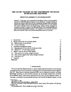
For the computational work we select the following examples from [7, 8, 10, 22]. Example 1. Let us consider the following nonlinear differential equation ) (( ) ∂u ∂ 1 −t ∂u 7 − e u + (t + 5) e−t = − t−9, (x, t) ∈ [0, 1]×[0, 1] (19) ∂t ∂x 6 ∂x 3 which has the exact solution u(x, t) = x2 et + t. In (19) ϕ(x, t) = − 73 t − 9, κ(t) = 61 e−t , ω(t) = (t + 5)e−t . In Table1, relative errors at different time levels are compared with the relative errors obtained by Zakeri et al. in [10]. In Figures 1 and 2 exact and numerical solutions are depicted. Example 2. Relative errors at different time levels are compared with the relative errors obtained by Nourazar et al. [8]. for Eq. (5) with α = 3, β = −4, n = 3, a = 0, b = 1√and t = √1 in Table 2. The exact solution of this example is υ(x, t) =

3 4

6x e( √

√ e 6x +e

6 x− 9 t 2 2

)

. The graph of the

exact and numerical solution, are shown in Figures 3 and 4. Table 1: Comparison of relative errors obtained from proposed method and method in [10].

x

Relative errors of proposed method

——————————————–

Relative errors obtained in [10]

——————————————

t = 0.25

t = 0.50

t = 0.75

t = 0.25

t = 0.50

t = 0.75

0.2

8.0999e-08

6.6631e-08

6.9815e-08

2.7500e-08

4.7700e-09

3.4500e-08

0.4 0.6

1.0121e-07 8.1254e-08

9.3251e-08 8.1761e-08

1.0112e-07 9.1375e-08

4.8100e-07 2.2800e-06

4.3300e-07 2.2700e-06

2.8500e-07 1.9100e-06

0.8 |e|1

4.4684e-08 6.4079e-08

4.7547e-08 5.9977e-08

5.4249e-08 6.5621e-08

6.7100e-06 –

6.7700e-06 –

5.8700e-06 –

From the test examples, we can say that the BSQI scheme is feasible and the accuracy is better than the multi-quadric quasi-interpolation (MQQI) method [6]. Moreover, MQQI method has very close relation to the shape


69

Table 2: Comparison of errors of Example 2 with the errors obtained in [8].(h = 0.02, τ = 0.0001)

x

Relative errors of proposed method

Relative errors obtained in [8]

——————————————————– t = 0.1

t=1

——————————————–

t = 0.15

t = 0.2

0.2

4.7533e-06

6.0414e-06

6.6041e-06

5.2440e-07

4.9987e-06

t = 0.1

5.6384e-05

3.1193e-04

0.4 0.8

6.8110e-06 4.7680e-06

8.4592e-06 5.4354e-06

9.1422e-06 5.6195e-06

7.1097e-07 4.0217e-07

6.3997e-06 3.6819e-06

6.8760e-05 3.7324e-05

3.6460e-04 1.8700e-04

|e|1

4.8486e-06

5.8747e-06

6.2722e-06

4.7741e-07

–

t = 0.15

t = 0.2

–

–

Figure 1: The exact solution of Example 1 for h = 0.02, τ = 0.00001

parameter c in MQ. In fact, the choice of the shape parameter is still a pendent question. Furthermore, the MQQI is required to calculate derivatives of MQ quasi interpolant once for all, which is not easy to compute when h is small. Although the accuracy of BSQI is not better than that of other methods, we know that, at each time step, the complexity of BSQI is lower than theirs. The proposed method is an acceptable and valid scheme. Moreover, it can be implemented very easily.

4 Conclusions In this article, we have applied the cubic B-spline quasi-interpolation method for solving the nonlinear Cauchy diffusion problem and NewellWhitehead equation. The results have been compared with the exact solutions and demonstrated the good performance of the schemes. This method offers several advantages in reducing computational costs. On the other hand, this method is very simple to apply and to make an algorithm. Thus, this method may be reckoned as a simple and accurate solver for PDEs and it is worthy to note that this method can be utilized as an accurate algorithm to solve linear and nonlinear functional equations arising in physics and other

70


Figure 2: The numerical results of Example 1 for h = 0.02, τ = 0.00001

Figure 3: The exact solution of Example 2 for h = 0.02, τ = 0.0001

fields of applied mathematics. The computations associated with the examples in this article were performed using MATLAB R2013a.

References 1. Burgers, J. M. The Nonlinear Diffusion Equation, Reidel Publishing Company, 1973. 2. Chen, R. and Wu, Z. Solving partial differential equation by using multiquadric quasi-interpolation, Applied Mathematics and Computation, 186 (2007) 1502-1510. 3. Chen, Z., Huan, G. and Ma, Y. Computational Methods for Multiphase Flows in Porous Media, Computational Science and Engineering, Society for Industrial and Applied Mathematics, Philadelphia, Pa, USA, 2006.


71

Figure 4: The numerical results of Example 2 for h = 0.02, τ = 0.0001

4. Cunningham, R. E. and Williams, R.J.J. Diffusion in Gasses and PorousMedia, Plenum Press, New York, NY, USA, 1980. 5. Dosti, M. and Nazemi, A.R. Solving one-dimensional hyperbolic telegraph equation using cubic B-spline quasi-interpolation, International Journal of Mathematical and Computer Sciences, 7 (2011) 57-62. 6. El-Hawary, H.M. and Mahmoud, S.M. Spline collocation methods for solving delay-differential equations, Applied Mathematics and Computation, 146 (2003) 359372. 7. Ezzati, R. and Shakibi, K. Using Adomian’s decomposition and multiquadric quasi-interpolation methods for solving newell-whitehead equation, Procedia Computer Science, 3 (2011) 1043-1048. 8. Farin, G. Curves and Surfaces for CAGD, fifth ed., Morgan Kaufmann, San Francisco, 2001. 9. Goh, J., Ahmad Abd. Majid, Ahmad Izani Md. Ismail, A quartic Bspline for second-order singular boundary value problems, Computers and Mathematics with Applications, 64 (2012), 115120. 10. J¨ ager, W., Rannacher, R. and Warnatz, J. Reactive Flows, Diffusion and Transport, Springer, Berlin, Germany, 2007. 11. Kadalbajoo, M.K., Tripathi, L.P. and Kumar, A. A cubic B-spline collocation method for a numerical solution of the generalized Black-Scholes equation, Mathematical and Computer Modelling, 55 (2012) 14831505. 12. K¨ arger, J. and Heitjans, P. Diffusion Condesed Matter, Springer, Berlin, Germany, 2005. 13. Khuri, S.A. and Sayfy, A. A spline collocation approach for a generalized parabolic problem subject to non-classical conditions, Applied Mathematics and Computation, 218 (2012) 91879196.

72


14. Kolokoltsov, V. Semi Classical Analysis for Diffusion and Stochastic Processes, Springer, Berlin, Germany, 2000. 15. Matinfar, M., Eslami, M. and Saeidy, M. An efficient method for Cauchy problem of ill-posed nonlinear diffusion equation, International Journal of Numerical Methods for Heat and Fluid Flow, 23 (2013) 427-435. 16. Mehrer, H. Diffusion Solids Fundamentals Methods Materials Diffusion Controlled Processes, Springer, Berlin, Germany, 2007. 17. Mittal, R.C. and Jain, R.K. Numerical solutions of nonlinear Burgers’ equation with modified cubic B-splines collocation method, Applied Mathematics and Computation, 218 (2012) 7839-7855. 18. Nourazar, S.S., Soori, M. and Nazari-Golshan, A. on the exact solution of Newell-Whitehead-Segel equation using the Homotopy Perturbation Method, Australian Journal of Basic and Applied Sciences, 5 (2011) 1400-1411. 19. Sablonnire, P. Univariate spline quasi-interpolants and applications to numerical analysis, Rendiconti del Seminario Matematico, 63 (2005) 211222. 20. Schumaker, L.L. Spline Functions: Basic Theory, third ed., Cambridge University Press, 2007. 21. V’azquez, J. L. The Porous Medium Equation, Oxford Mathematical Monographs, The Clarendon Press, Oxford, UK, 2007. 22. Yuab, R.G., Wanga, R.H. and Zhu, C.G. A numerical method for solving KdV equation with multilevel B-spline quasi-interpolation, Applicable Analysis: An International Journal, 92 (2012) 1682-1690. 23. Zakeri, A., Aminataei, A. and Jannati, Q. Application of He’s Homotopy Perturbation Method for Cauchy Problem of Ill-Posed Nonlinear Diffusion Equation, Discrete Dynamics in Nature and Society, Volume 2010, Article ID 780207, 10 pages. 24. Zhu, C.G. and Kang, W.S. Applying Cubic B-Spline Quasi-Interpolation To Solve Hyperbolic Conservation Laws, U.P.B. Sci. Bull., Series D, 72 (2010) 49-58. 25. Zhu, C.G. and Kang, W.S. Numerical solution of Burgers-Fisher equation by cubic B-spline quasi-interpolation, Applied Mathematics and Computation, 216 (2010) 26792686. 26. Zhu, C.G. and Wang, R.H. Numerical solution of Burgers’ equation by cubic B-spline quasi-interpolation, Applied Mathematics and Computation, 208 (2009) 260272.

‫ﻣﻄﺎﻟﻌﻪ ﻋﺪدي ﻣﺴﺄﻟﻪ ﻏﻴﺮ ﺧﻄﻲ ﮐﻮﺷﻲ و ﻣﻌﺎدﻟﻪ ﻧﻴﻮﻳﻞ‪-‬واﻳﺘﻬﺪ ﺑﺎ روش ﺷﺒﻪ دروﻧﻴﺎب ﺑﻲ‪-‬اﺳﭙﻼﻳﻦ‬ ‫ﻣﮑﻌﺒﻲ‬ ‫ﺣﺴﻴﻦ اﻣﻴﻨﻲ ﺧﻮاه و ﺟﻮاد ﻋﻠﻮي‬ ‫داﻧﺸﮕﺎه ﮔﻴﻼن‪ ،‬داﻧﺸﮑﺪه ﻋﻠﻮم رﻳﺎﺿﻲ‪ ،‬ﮔﺮوه رﻳﺎﺿﻲ ﮐﺎرﺑﺮدي‬

‫ﭼﮑﯿﺪه ‪ :‬اﻳﻦ ﻣﻘﺎﻟﻪ ﺑﻪ ﻣﻄﺎﻟﻌﻪ ﻳﮏ ﺗﻘﺮﻳﺐ ﻋﺪدي از ﻣﻌﺎدﻟﻪ ﻧﻴﻮﻳﻞ‪-‬واﻳﺘﻬﺪ و ﻣﻌﺎدﻟﻪ ﺑﺪوﺿﻊ اﻧﺘﺸﺎر ﮐﻮﺷﻲ‬ ‫ﻣﻲﭘﺮدازد‪ .‬در ﻃﺮح اراﺋﻪ ﺷﺪه از ﻣﺸﺘﻖ ﺑﻲ‪-‬اﺳﭙﻼﻳﻦ ﺷﺒﻪ دروﻧﻴﺎب ﺑﺮاي ﺗﻘﺮﻳﺐ ﻣﺸﺘﻖ ﻣﺘﻐﻴﺮﻫﺎي واﺑﺴﺘﻪ و‬ ‫از ﺗﻔﺎﺿﻞ ﭘﻴﺸﺮو ﻣﺮﺗﺒﻪ اول ﺑﺮاي ﺗﻘﺮﻳﺐ ﻣﺸﺘﻖ زﻣﺎن اﺳﺘﻔﺎده ﻣﻲﺷﻮد‪ .‬ﻣﺜﺎلﻫﺎﻳﻲ ﺑﺮاي ﺗﺸﺮﻳﺢ روش ﺑﻴﺎن‬ ‫ﺷﺪه و ﻧﺘﺎﻳﺞ ﻋﺪدي ﻣﺜﺎلﻫﺎ ﺑﺎ ﺟﻮابﻫﺎي دﻗﻴﻖ ﻣﻘﺎﺳﻴﻪ ﺷﺪهاﻧﺪ‪ .‬ﻣﺰﻳﺖ اﺻﻠﻲ اﻳﻦ روش در اﻟﮕﻮرﻳﺘﻢ و ﭘﭙﺎده‬ ‫ﺳﺎزي ﺳﺎده آن اﺳﺖ‪.‬‬ ‫ﮐﻠﻤﺎت ﮐﻠﯿﺪی ‪ :‬ﺷﺒﻪ دروﻧﻴﺎب ﺑﻲ‪ -‬اﺳﭙﻼﻳﻦ ﻣﮑﻌﺒﻲ؛ ﻣﻌﺎدﻟﻪ اﻧﺘﺸﺎر‪ -‬اﻧﺘﻘﺎل؛ ﻃﺮح ﺗﻔﺎﺿﻠﻲ‪.‬‬

Numerical study of the nonlinear Cauchy diffusion problem and

Numerical study of the nonlinear Cauchy diffusion problem and

Suggest Documents