Jan 25, 2016 - present integer programming models that can be used to design numerically balanced dice. .... Is there a
Numerically Balanced Dice Robert Bosch, Robert Fathauer, and Henry Segerman January 25, 2016 Abstract We discuss what it might mean for a die to be numerically balanced, explore connections with magic squares, and present integer programming models that can be used to design numerically balanced dice.
Introduction On most commercially available twenty-sided dice (d20s), the numbers on opposite sides sum to 21. This is true for the d20 shown in Figure 1(a), manufactured by Chessex, which has the 8 opposite the 13, the 20 opposite the 1, the 10 opposite the 11, and so on. Why do die manufacturers do this? To answer this question, let’s perform a thought experiment. Suppose we get our hands on a perfectly fair d20, a regular icosahedron. We heat it up to make it soft, and then we carefully position it in a vice or a clamp, as in Figure 1(b), making sure that one of the faces lies flat against one jaw and that the opposite face lies flat against the other jaw. Then, with every turn of the crank, the jaws move closer and closer together, squeezing the two “jaw faces” closer and closer to each other, and making the once-fair d20 flatter and flatter, less and less of a regular icosahedron, and more and more like a coin. And with every turn of the crank, the d20 will become less fair. If we are careful with the squeezing, each jaw face will continue to be as likely to turn up as the other jaw face, but each jaw face will also become more likely to turn up than any of the 18 non-jaw faces. Still, if the numbers on opposite faces sum to 21, then the expected value of a single roll of the squashed d20 will remain 10.5, the value for a fair d20 (the average of the numbers 1 through 20). So the squashed d20 won’t systematically favor higher-than-average or lower-than-average numbers.
Figure 1: (a) a d20 and its reflection in a mirror, (b) squeezing a d20. Our thought experiment reveals that the opposite numbers convention is a form of “numerical balancing” that serves to promote fairness, giving die manufacturers a way of hedging against the possibility that their d20s are not perfectly formed regular isocahedra. Are there additional measures that they could take? Is it possible to make d20s that are even more numerically balanced?
Vertex Sums For each vertex of a d20, we can compute the vertex sum—the sum of the numbers on the five faces that meet at that vertex. If a d20’s numbers were uniformly spread amongst its twenty faces, then each vertex sum would be 52.5 = 5 × 10.5, five times the average of the numbers on the die. If all twelve of a d20’s vertex sums are as close to 52.5 as possible (i.e., all of its vertex sums are 52 or 53), we say that it has numerically balanced vertices. Having numerically balanced vertices could provide additional protection against certain manufacturing imperfections and irregularities. Let’s perform a second thought experiment: Suppose that the d20 shown in Figure 1 contains a large air bubble that lies just beneath the vertex formed by the faces numbered 1, 13, 5, 15, and 7. With the bubble-vertex side of the d20 being less dense than the rest of the die, its faces may be more likely to turn up than the others. If so, the die would tend to produce lower numbers than a fair d20 would. The reason why is that the bubble vertex’s vertex sum, 1 + 13 + 5 + 15 + 7 = 41, is considerably lower than the ideal vertex-sum value, 52.5. Face Sums Similarly, for each face of a d20, we can compute the face sum—the sum of the numbers on the three faces that are adjacent to that face. If a d20’s numbers were uniformly spread amongst its twenty faces, then each face sum would be 31.5, three times the average of the numbers on the die. If all twenty of a d20’s face sums are as close to 31.5 as possible (i.e., all of its face sums are 31 or 32), we say that it has numerically balanced faces. Having numerically balanced faces could provide even more protection against manufacturing defects. For a third thought experiment, suppose that an air bubble lies just below the face numbered 13 and suppose in addition that there is a small bump on the surface of the opposite face. These two defects may cause the numbers adjacent to the 13—the 1, the 11, and the 5—to turn up with greater frequency than the other numbers. If so, the die will once again favor lower numbers. Here, the reason is that the face sum of 1 + 11 + 5 = 17 is substantially lower than the ideal face-sum value, 31.5. Full Face Sums Alternatively, for each face of a d20, we could compute the full face sum—the sum of the numbers on the three faces adjacent to that face plus the number on that face itself. Although it may seem preferable— for aesthetic or geometric reasons—to use full face sums when defining numerically balanced faces, doing so turns out to be problematic. Consider a cube, and consider numbering it to form a d6. If we follow the opposite numbers convention, keeping the 6 opposite the 1, the 5 opposite the 2, and the 4 opposite the 3, then there are two possible numberings, and they are mirror images of each other. In each of these numberings, each face has the same face-sum value, 14, as the four adjacent faces will always contain two pairs of opposite faces whose numbers sum to 7. But in each of these numbering, each face does not have the same full-face-sum value. Instead, there are six different full-face-sum values: 15, 16, 17, 18, 19, and 20. (The 15 is the full-face sum for the 1, the 16 is the full-face sum for the 2, and so on.) Thus, for a d6, if we are committed to following the opposite numbers convention, there is no way of making all of its full face sums the same. This is also true for a d20. The methods we describe later in this paper can be used to show that if we number a d20 in accordance with the opposite numbers convention, there is no way of making all of its full face sums the same. Equatorial Bands If we select a vertex to serve as a d20’s north pole, then its opposite vertex must be its south pole. The five faces adjacent to the north pole form the northern polar cap, and the five adjacent to the south pole form the southern polar cap. The remaining ten faces—five pairs of opposite faces—form an equatorial band that
encircles the d20. Figure 2 displays two views of one of the ten possible equatorial bands.
Figure 2: Two views of an equatorial band. A net enables us to see all twenty faces of a d20 at once. In Figure 3, the top and bottom rows of the net are the two polar caps shown in Figure 2, and the middle row is the corresponding equatorial band. For each possible equatorial band, we can compute the band sum—the sum of the numbers on the faces that make up the band. But in this case we don’t need to do so. If a d20 obeys the opposite numbers convention, then each of its band sums must be 105, as each band is made of five pairs of opposite faces whose two numbers sum to 21. In other words, if a d20 obeys the opposite numbers convention, then it must have numerically balanced equatorial bands. And numerically balanced equatorial bands are desirable. Let’s perform one final thought experiment. Suppose that during the manufaturing process, one particular north-pole-south-pole pair is farther apart that it should be, making the d20 somewhat cigar shaped. If so, the faces on the equatorial band would turn up more often the others. But if each band sum is 105, then the expected value of a single roll will remain 10.5. 1 1
2
3
4
5
15
7
17
10
12
2
3
4
5
6
6
5
8
1
10
3
12
8
14
2
18
7
13
9
19
11
16
13
20
15
7
8
9
10
11
4
11
9
6
14
16
17
18
19
20
12
Figure 3: A net for the Chessex d20. This is a common numbering and is typical of that used by other manufacturers. The Chessex d20—the one shown in the photos and net—obeys the opposite numbers convention and therefore has numerically balanced equatorial bands. We have already demonstrated—by computing a single vertex sum and a single face sum—that it has neither numerically balanced vertices nor numerically balanced
faces. With the net—which gives the numbers that index the faces and vertices in a small gray font, and the numbering itself in a larger black font—we can quickly verify that this d20 is not even remotely close to having numerically balanced vertices or faces. Only four of the vertex sums—those that are underlined—are as close as possible to the ideal vertex-sum value, 52.5: vertex index vertex sum
1 61
2 52
3 41
4 47
5 54
6 52
7 51
8 53
9 53
10 64
11 58
12 44
And none of the face sums are as close as possible to the ideal face-sum value, 31.5: 1 24
face index face sum face index face sum
6 11
7 46
8 17
face index face sum
2 33 9 39
16 43
3 20 10 13
17 26
4 37 11 52
18 36
5 27 12 17
19 39
13 46
14 24
15 50
20 30
Several natural questions arise: Is there a better (more numerically balanced) d20? Is there a best (most numerically balanced) d20? This last question can be rephrased as follows: Does there exist a d20 that obeys the opposite numbers convention and has both numerically balanced vertices and faces? What about other polyhedral dice?
Magic Squares The problem of finding a numerically balanced d20 is similar to the problem of finding a magic square. An order-n magic square is an n × n array that contains the integers 1 through n2 and whose rows, columns, and main diagonals all sum to the same number c = (n3 + n)/2. Two renditions of an order-4 magic square are displayed below. The version made out of LEGO demonstrates that magic squares are not only numerically balanced, but can be used to form physically balanced structures as well.
1
8
13
12
14
11
2
7
4
5
16
9
15
10
3
6
Figure 4: (a) an order-4 magic square, (b) the same square made out of LEGO.
The problem of finding an order-n magic square can be formulated as an integer program (IP). Integer programs are mathematical optimization problems in which the objective is to optimize (in some cases, to maximize, and in others, to minimize) a linear function of integer-valued variables subject to one or more linear constraints (equations or inequalities) on those variables [10]. Since the 1960s, integer programs have been applied with great frequency and success to problems in the areas of logistics, manufacturing, and scheduling, and in these applications, the objective is usually to maximize profit or minimize cost [4]. But integer programs have also been used to solve puzzles [1,5], investigate cellular automata [2], and transform target images into mosaics and continuous line drawings [3]. When modeling the magic square problem as an IP, the natural starting point is to define a variable xi,j to represent the as-yet-unknown number that will be placed in cell (i, j), the cell in row i and column j of the array. With these variables, it is easy to express the constraints on the row sums, the column sums, and the two diagonal sums with linear equations: n X j=1 n X i=1 n X
xi,j
= c
for each 1 ≤ i ≤ n,
(1)
xi,j
= c
for each 1 ≤ j ≤ n,
(2)
and
(3)
xi,i = c
i=1 n X
xi,n+1−i = c.
(4)
i=1
The difficulty is finding a way of forcing all of the xi,j values to be different from one another using only linear equations or inequalities. One standard approach introduces binary variables (
yi,j,k =
1 if xi,j = k, 0 if not,
along with the following linear equations: n X n X
yi,j,k = 1
for each 1 ≤ k ≤ n2 ,
(5)
yi,j,k = 1
for each 1 ≤ i ≤ n, 1 ≤ j ≤ n,
(6)
k yi,j,k = xi,j
for each 1 ≤ i ≤ n, 1 ≤ j ≤ n.
(7)
i=1 j=1 2
n X k=1 2
n X k=1
The equations in (5) and (6) are known as assignment constraints. They state that each number between 1 and n2 must be placed in a cell and that each cell (i, j) must receive a number. The equations in (7) establish links between the xi,j variables and the yi,j,k variables. They make sure that xi,j = k if and only if yi,j,k = 1. No objective function is needed—the magic square problem is a feasibility problem, a constraint satisfaction problem—but we can create a dummy objective function by defining dummy costs ci,j,k = 0 for all 1 ≤ i ≤ n, 1 ≤ j ≤ n, 1 ≤ k ≤ n2 . Or if we have in mind a meaningful non-zero objective function—perhaps we want to make the sum of the interior cell numbers as small as possible—we can compute appropriate values for the ci,j,k coefficients. Regardless, to obtain our magic square, we then solve the
following IP: 2
minimize
n X n X n X
ci,j,k yi,j,k
i=1 j=1 k=1
subject to
constraints (1) through (7), xi,j ∈ {1, 2, . . . , n2 }
for each 1 ≤ i ≤ n, 1 ≤ j ≤ n
yi,j,k ∈ {0, 1}
for each 1 ≤ i ≤ n, 1 ≤ j ≤ n, 1 ≤ k ≤ n2 .
Finding Numerically Balanced d20s The problem of finding a numerically balanced d20 can also be formulated as an IP. Notation Here, we let F denote the set of faces of the d20 and V the set of vertices. For each v ∈ V , we let Pv denote the set of five faces that meet at vertex v. The faces in Pv form a pentagonal cap centered at v. For each f ∈ F , we let Af denote the set of three faces that are adjacent to face f . Finally, for each f ∈ F , we let O(f ) stand for the face that is opposite face f . Variables As in the magic squares model, we have two sets of variables. For each f ∈ F , we let xf equal the number assigned to face f . For each f ∈ F and each 1 ≤ k ≤ 20, we let yf,k = 1 if xf = k and 0 if not. A Nonlinear Model minimize
X X xf 0 ) − 31.5 (
subject to
20 X
(8)
f 0 ∈Af
f ∈F
yf,k = 1
for each f ∈ F ,
yf,k = 1
for each 1 ≤ k ≤ 20,
(10)
k yf,k = xf
for each f ∈ F
(11)
xf + xO(f ) = 21
for each f ∈ F
(12)
X
xf ≤ 53
for each v ∈ V
(13)
xf ∈ {1, 2, . . . , 20}
for each f ∈ F
(14)
yf,k ∈ {0, 1}
for each f ∈ F and each 1 ≤ k ≤ 20.
(15)
(9)
k=1
X f ∈F 20 X k=1
52 ≤
f ∈Pv
The objective function, (8), is the sum of twenty nonnegative error terms, one per face. For each face f ∈ F , we define the face-sum deviation to be the face sum minus the ideal face-sum value, 31.5. Note that the face-sum deviation could be negative. We define the error for face f to be the absolute value of its face-sum deviation. By minimizing the sum of the errors—the sum of the absolute values of the face-sum deviations—we are searching for a numbering that has numerically balanced faces. The constraints in (9), (10), and (11) are analogous to (5), (6), and (7) in the magic square model. The equations in (9) and (10) are assignment constraints that force us to give each face a number from 1 to 20
and to use each of these numbers exactly once, and the equations in (11) are linking constraints that make sure that xf = k if and only if yf,k = 1. Finally, the constraints in (12) and (13) ensure that model generates a numbering that obeys the opposite numbers convention and has numerically balanced vertices. A Linear Model Instead of trying to tackle the nonlinear model we just described—the absolute value error terms in the objective function make it nonlinear—we solve a related model that has a linear objective function. To “linearize” the original objective function (8), we can introduce a continuous variable zf to stand in for face f ’s error term in (8) and then impose two lower bounds on each zf : X
zf ≥ (
xf 0 ) − 31.5
(16)
f 0 ∈Af
zf ≥ 31.5 − (
X
xf 0 ).
(17)
f 0 ∈Af
Inequality (16) states that zf must be at least as big as face f ’s face-sum deviation, and inequality (17) states that zf must be at least as big as the negative of f ’s face-sum deviation. Combining (16) and (17) gives us n X
zf ≥ max (
X
xf 0 ) − 31.5, 31.5 − (
f 0 ∈Af
f 0 ∈Af
X
o
xf 0 ) = (
f 0 ∈Af
xf 0 ) − 31.5 .
If we minimize the sum of the zf variables subject to (16) and (17) and all of the previous constraints, then in the optimal solution, zf will equal the error for face f . Results We solved the linearized model—a mixed integer program due to the continuous zf variables—with branch and bound, a divide-and-conquer strategy that tackles an IP or mixed IP by constructing a binary tree of linear programming (LP) relaxations. We used Gurobi Optimizer 6.0.0 [8] to perform the branch and bound, and it needed only 0.13 seconds and a total of 5479 iterations of the simplex algorithm to find a optimal solution and prove its optimality. The branch-and-bound tree had 362 nodes. Figure 5 displays the optimal solution. Using this net, it is easy to verify that six of the twelve vertices have vertex sums of 52, and the remaining six—the opposite vertices—have vertex sums of 53. vertex index vertex sum
1 52
2 52
3 53
4 53
5 52
6 52
7 53
8 53
9 53
10 52
11 52
12 53
And it is also easy to check that ten of the twenty faces have face sums of 31, and the other ten—the opposite faces—have face sums of 32. 1 32
face index face sum face index face sum
6 32
7 31
face index face sum
8 32
2 31 9 32
16 31
3 32 10 32
17 32
4 31 11 31
18 32
5 31 12 32
19 31
13 31
14 31
15 31
20 32
Accordingly, the optimal numbering has numerically balanced faces and vertices. Figure 6 shows five copies of our numerically balanced d20, the first of its kind (to our knowledge). They are available from The Dice Lab [6].
1 1
2
3
4
5
11
1
15
13
12
2
3
4
5
6
6
19
8
5
10
18
12
4
14
7
3
7
17
9
14
11
2
13
16
15
7
8
9
10
11
6
8
9
10
20
16
17
18
19
20
12
Figure 5: A net for the optimal solution.
Figure 6: Five copies of The Dice Lab’s numerically balanced d20.
Other Dice The definitions and models can be modified for other polyhedral dice. Some of the most commonly used dice—the d4, d6, d8, d12, and d20—are based on the five platonic solids. In a platonic solid, each vertex is the same degree (each is touched by the same number of faces). But for other polyhedra, this isn’t necessarily the case. The rhombic triacontahedron, for example, is a polyhedron that has 30 faces and 32 vertices. Twenty of the vertices are degree 3, and the remaining twelve have degree 5. For a d30 based on the rhombic triacontahedron, opposite faces should sum to 31. Ideally, each degree-3 vertex would have a vertex sum of 46.5 = 3 × 15.5, three times the average of the numbers from 1 to 30, and each degree-5 vertex would have a vertex sum of 77.5 = 5 × 15.5, five times the average. The diskyakis triacontahedron is a polyhedron that has 120 faces and 62 vertices. Thirty of the vertices
are degree 4, twenty are degree 6 and the remaining twelve are degree 10. For a d120 based on the diskyakis triacontahedron, opposite faces should sum to 121. Ideally, each degree-4 vertex would have a vertex sum of 242 = 4 × 60.5, four times the average of the numbers from 1 to 120. For the degree-6 and degree-10 vertices, the corresponding values are 363 = 6 × 60.5 and 605 = 10 × 60.5. To be suitable as a die, a polyhedron must be isohedral. Its symmetry group must be transitive on its faces [7]. The platonic solids are isohedral and so are the rhombic triacontahedron and the diskyakis triacontahedron. The isohedral property ensures fairness, guaranteeing that each face is equally likely to turn up provided that (1) the die is a physically perfect rendition of the polyhedron, and (2) the toss does an ideal job of sampling from the set of available states [9]. Of course, in the real world, neither of these two conditions is ever realized. And this is why numerical balancing is so important. As mentioned earlier, it gives die manufacturers ways of hedging against the possiblity (rather, the certainty) of bias caused by imperfections in manufacturing. If the number of faces, n, is small, then there is no need for integer programming or any other computationally intensive methods. With pencil and paper, one can enumerate all numberings of a d4, d6, d8, and if one has a lot of patience, a d12. (And The Dice Lab does offer an optimally numbered d8, the only one on the market, as far as we are aware.) One could employ brute-force enumeration to investigate all possible numbers of a d20, but if we want to number polyhedra with even more faces, brute-force enumeration becomes less and less appealing and our IP model becomes more and more of an attractive tool. A Balanced d30 Here, the set of vertices V is the union of two disjoint sets, V3 (the set of degree-3 vertices) and V5 (the set of degree-5 vertices). For each v ∈ V3 , we let Hv equal the set of three faces that are adjacent to vertex v. In a rhombic triacontahedron, each set Hv forms a hexagonal region. For each v ∈ V5 , we let Sv equal the set of five faces that are adjacent to vertex v. In the rhombic triacontahedron, each set Sv is star shaped.
Figure 7: Two views of a (virtual) numerically balanced d30. For the d30, we did not try to balance face sums. The reason is that we judged the sets of four faces that are adjacent to a particular face to be somewhat strange in appearance. Ignoring the face sums, we modified the approach we used in the d20 case to search for a numbering that obeys the opposite numbers convention and has vertex sums that are as close to being balanced as possible. We did this by solving the linearization of the following model: minimize
X X X X xf ) − 46.5 + xf ) − 77.5 ( ( v∈V3
subject to
f ∈Hv
v∈V5
f ∈Sv
the assignment, linking, and opposite-numbers constraints.
Using Gurobi, we obtained an optimal solution that corresponds to the numerically balanced d30 shown in Figure 7. On this problem, Gurobi required 2.36 seconds and a total of 77328 simplex algorithm iterations
to solve the LP relaxations at the 3442 nodes of the branch-and-bound tree. All of these statistics are quite a bit higher than those in the d20 problem. A Balanced d120 We began this entire project because we were interested in numbering a 120-sided die based on a diskyakis triacontahedron. The diskyakis triacontahedron can be obtained by turning each face of a rhombic triacontahedron into a pyramid with a rhombus as its base. Three half pyramids come together to form equilateral triangles comprised of six faces. Twenty of these triangles are arranged in icosahedral fashion, as shown in Figure 8. As mentioned earlier, the polyhedron has 120 faces and 62 vertices. Thirty of the vertices are degree 4 (the black dots), twenty are degree 6 (the gray dots), and the remaining twelve are degree 10 (the white dots).
Figure 8: A schematic for a 120-sided die. Here, the set of vertices V is the union of three disjoint sets: V4 (the set of degree-4 vertices), V6 (the set of degree-6 vertices), and V10 (the set of degree-10 vertices). For each v ∈ V4 , we let Qv denote the set of four faces that meet at v. The faces in Qv form a quadilateral-shaped cap centered at v. For each v ∈ V6 , we let Hv denote the set of six faces that meet at v. The faces in Hv form a hexagonal cap centered at v. And for each v ∈ V10 , we let Dv denote the set of ten faces that meet at v. The faces in Dv form a decagonal cap centered at v. In an effort to search for a numbering that has numerically balanced vertices, once again ignoring face sums for the same reason as in the d30, we attempted to solve a linearization of the following nonlinear model: minimize
X X X X X X xf ) − 242 + xf ) − 363 + xf ) − 605 ( ( ( v∈V4
subject to
f ∈Qv
v∈V6
f ∈Hv
v∈V10
f ∈Dv
the assignment, linking, and opposite-numbers constraints.
We found that Gurobi was not able to solve the full mixed integer program for the d120. After several days of branch and bound, the branch-and-bound tree still had tens of millions of unexplored nodes (and was still growing). Fortunately, after all of this computation, Gurobi was able to find a solution that was very close to having numerically balanced vertices. All of the degree-10 vertices had vertex sums of 605, and all of the degree-6 vertices had vertex sums of 363. Moreover, 28 of the 30 degree-4 vertices had vertex sums
of 242. Unfortunately, two of the degree-4 vertices were off by 2. One had a vertex sum of 240, a deviation of −2, and the other one (its opposite on the d120) had a vertex sum of 244, a deviation of +2. At this point, we tried various forms of IP-based local search. In the final (successful) version, starting from our error-4 solution, we randomly picked a face and “grew” the face, selecting its neighbors, all of its neighbors’ neighbors, and all of its neighbors’ neighbors’ neighbors. We kept all of the variables that corresponded to the selected faces fixed at their values in the error-4 solution, and we used Gurobi to solve the reduced model, allowing it to do its best with the unfixed variables. We did this repeatedly. And after dozens of hours, Gurobi found a solution with error 0, a solution with numerically balanced vertices. The solution is shown in Figure 9, and a photo of the physical object is shown in Figure 10.
62 33 27 78
71
73
20
98
3
92
37
49 11
61
102
16
75
34
51 85
90
5
117
46
58 22
15
109
21
103
9
57
96
66 32
64
67
76
6
83
77
79
65
35 24
42 38
12 100
41
111
1
84
48
101
43
50
94
29
59 88
54
17 119 8
23
56 44
45 115
106
68 39 72 110
120
86 97
25
18 112
60
13 81 104 2
10
55 89
87
19 105
107
113 95
80
63
70 36
52
30
28
53 82 99
74
114
26
108 40 93
14
116
4
91
31
7
69
118 47
Figure 9: A schematic for the numerically balanced d120.
Figure 10: The Dice Lab’s numerically balanced d120.
Conclusions Many if not most of the polyhedral dice on the market today are not numbered in as balanced a manner as possible. This could be due to the use of historical numberings that may predate the wide use of computers. In our view, there is no good reason to continue using these antiquated numberings. We have described both the rationale and a method for creating new and improved numberings. Future work includes the application of these methods to additional polyhedral dice. Studies could be carried out to determine the most common sources of bias for different kinds of dice. The results of such studies would aid in prioritizing the importance of different types of numerical balancing.
References [1]
A. Bartlett, T.P. Chartier, A.N. Langville, and T.D. Rankin, An integer programming model for the Sudoku problem, J. of Online Mathematics and its Applications 8 (2008). [2] R.A. Bosch, Integer programming and Conway’s game of Life, SIAM Review 41:3 (2006), pp. 594604. [3] R. Bosch. Opt art, Math Horizons Feb. (2006), pp. 6-9. [4] D.-S. Chen, R.G. Batson, and Y. Dang, Applied Integer Programming: Modeling and Solution, Wiley, 2010. [5] M.J. Chlond, Classroom exercises in IP modeling: Su doku and the log pile, INFORMS Transactions on Education 5:2 (2005), pp. 77-79. [6] The Dice Lab, Numerically-balanced d20 page, available at http://thedicelab.com/BalancedStdPoly.html, January 2016. [7] P. Diaconis and J.B. Keller, Fair Dice, The American Mathematical Monthly 96:5 (1989), pp. 337-339. [8] Gurobi Optimization, Inc., Gurobi Optimizer Reference Manual, availabe at http://www.gurobi.com, January 2016. [9] B. Thurston, http://mathoverflow.net/questions/46684/fair-but-irregular-polyhedral-dice (accessed 1/25/16). [10] L. Wolsey, Integer Programming, Wiley-Interscience, 1998.