NYQUIST-RATE DETECTION OF CPM SIGNALS USING THE VITERBI ALGORITHM K. Vasudevan K. Giridhar and Bhaskar Ramamurthi Department of Electrical Engineering Indian Institute of Technology, Madras 600 036 e-mail:
[email protected]
Abstract This paper discusses Viterbi Algorithm (VA) based coherent and non-coherent sequence estimation for the detection of Continuous Phase Modulated (CPM) signals. It is well known that the VA for the coherent approach implements the MLSE. Previously published literature has only dealt with noncoherent block estimation techniques, since noncoherent MLSE does not easily lend itself to implementation using the VA. We propose a suboptimal non-coherent sequence estimation approach that uses the VA. By using Nyquist-rate samples of the complex baseband CPM signal, we avoid the need for a Whitened Matched Filter (WMF). We present theory and simulation results of the approaches discussed, for GMSK having a 3-dB bandwidth equal to half the bit-rate. An interesting result is that the VA-based suboptimal non-coherent approach performs nearly as well as the coherent MLSE.
1
Introduction
Continous Phase Modulation (CPM) is widely used in digital wireless communications. In this paper, we deal with the discrete-time VA-based detection of CPM signals, suitable for running on programmable DSP platforms. We consider only distortionless reception of the CPM signal at the receiver. Coherent MLSE of CPM signals using Viterbi detectors operating at symbol-rate is well understood [1]. Non-coherent detection of MSK using an MLSE-type algorithm operating on a block-by-block basis, has been described in [2]. Although this detector performs nearly as well as the coherent detector, its computational complexity is high, especially for large block sizes. One way to reduce the complexity of the MLSE is to employ the VA [1]. Since non-coherent MLSE for CPM does not lend itself to implementation using the VA, we propose a sub-
optimal non-coherent sequence estimation approach that uses the VA. This suboptimal non-coherent VA (SNVA) is shown to have an error-rate very similar to the coherent detector, with no additional complexity. In addition to the SNVA, the other important aspect in this paper is that the VA operates on the Nyquist-rate samples of the received signal. When the VA is used for detection, the performance of the coherent and non-coherent approaches is governed by the minimum distance error event. For the particular case of GMSK having a 3-dB bandwidth equal to half the bit-rate, we show using the concept of minimum distance error event, that the probability of bit error at high SNR for the coherent and non-coherent approaches, are nearly the same.
2
Communication Model
A CPM signal can be written in the form s(t) = A cos(2πFc t + θ(t)).
(1)
The information is contained in the phase, θ(t), as given by Z t β(τ ) dτ, (2) θ(t) = 2πh 0
where β(τ ) is a Pulse Amplitude Modulated (PAM) signal. Hence β(τ ) can be written as β(τ ) =
bτ /T c
X
k=d(τ /T )−Le
b(kT )p(τ − kT ),
(3)
where b·c denotes the “floor”and d·e denotes the “ceil”. The symbols b(kT ) are drawn from an M ary PAM constellation, p(·) is a pulse shape which extends over L symbol durations in general, T corresponds to one symbol duration and h is termed as the modulation index, which is usually a ratio of two relatively prime integers.
In this paper we consider as an example a particular case of CPM namely, Gaussian Minimum Shift Keying (GMSK) [3] where b(kT ) ∈ {1, −1} and h = 0.5. The received CPM signal r(t) is assumed to be centered at FIF Hz and bandlimited to [FIF − W, FIF + W ] Hz. Typically FIF is much larger than the bit-rate (1/T ) and hence bandpass sampling [4, Chap. 7] is required to efficiently represent the continuous-time IF signal in terms of its samples. Also, for the purpose of efficient demodulation of the bandpass CPM signal, it is convenient to select FIF such that the magnitude spectrum of the sampled signal is centered at ±π/2. For ease of recovering the bit-stream we impose a restriction on the sampling frequency (Fs ) such that it is an integer multiple of the bit-rate. So, the discrete-time CPM signal can be written as r(n) = cos(ωc n + θi (n) + θ0 ) + w(n).
(4)
The radian frequency, ωc = 2πFIF /Fs and θi (n) denotes the phase at time n, due to the ith possible transmitted sequence. Note that if FIF /Fs = (2m + 1)/4, for some positive integer m, then ωc = (2m + 1)π/2, which is equivalent to a radian frequency of π/2. The term θ0 is a random phase that is possibly unknown at the receiver. Finally, w(n) denotes samples of a zero-mean white Gaussian noise process, w(t), having two-sided power spectral density N0 /2 watts/Hz. The variance of 2 w(n) is given by σw = 2N0 W . We follow the notation that a time index of n implies a sampling frequency of Fs , unless explicitly stated otherwise. We also assume that there are 2C samples every bit. The amplitude of the cosine term in the above equation is of little consequence in our analysis and is hence assumed to be unity for the sake of mathematical convenience. For the purpose of deriving the ideal MLSE approach, we shall assume that totally B bits are transmitted by the transmitter. Note that there are 2 B possible transmitted sequences.
3
MLSE-Based Coherent and Noncoherent Detection
Let us reconsider the CPM signal given in equation (4). This can be written in a modified form as follows: r(n) = cos(ωc n) cos(θi (n) + θ0 ) − sin(ωc n) sin(θi (n) + θ0 ) + w(n).
(5)
cos(nπ/2) αI (2nTs ) Delay
↓2
Interpolator
↓2
r(n)
αQ (2nTs ) − sin(nπ/2) Figure 1: Demodulating the CPM signal.
So r(n) can be demodulated like any other bandpass signal. Figure 1 shows an efficient method of demodulation. Let α(·) ˜ denote the complex baseband signal. It can be shown that [θi (2nTs )+θ0 ] α(2nT ˜ +u ˜(2nTs ), s ; θ0 ) = e
(6)
where the complex noise samples ∆
u ˜(2nTs ) = uI (2nTs ) + uQ (2nTs ).
(7)
The noise samples uI (2nTs ) and uQ (2nTs ) are 2 Gaussian with zero mean and variance σw . Assuming for the sake of mathematical convenience that the interpolator is ideal, it can be shown that the power spectral density of both uI (2nTs ) and uQ (2nTs ) is flat over [−π, π]. Note that the sampling frequency is now equal to Fs /2. The MLSE can now be performed on the complex baseband samples given by equation (6). In the next subsection we consider the coherent approach, where we assume that θ0 is equal to zero.
3.1
Coherent MLSE Approach
Here we assume without any loss of generality that θ0 = 0. So the complex baseband will be represented as α(2nT ˜ ˜ s ) instead of α(2nT s ; θ0 ), as in equation (6). The task of the ideal MLSE is to decide in favour of that sequence, which is nearest in the Euclidean sense, to the transmitted sequence. We assume that all sequences are equally likely. The distance computations for the coherent method take the form [5] Dj (BT ) =
2 θj (2nTs ) ˜ α(2nT s) − e
CB−1 X n=0
(8)
8.0
where the MLSE decides in favour of the minimum distance. Here T denotes the bit duration. Note that 0 ≤ j ≤ 2B − 1 and we have C samples per bit since the sampling frequency is Fs /2. Expanding the squares and simplifying, we get CB X
n=0
o n < α ˜ (2nTs )e−θj (2nTs )
(9)
Multiplicity
Mj (BT ) =
6.0
where the MLSE decides in favour of the maximum correlation. The noise samples, vj (2nTs ), in equation (9) are given by n o vj (2nTs ) = < u ˜(2nTs )e−θj (2nTs ) (10)
4.0
2.0
0.0 0.0
5.0
10.0
th
When the i possible sequence is transmitted, note that for j = i, equation (9) reduces to Mi (BT ) = CB, in the absence of noise. The metric Mj (BT ) in equation (9) can be recursively written as Mj (kT ) = Mj ((k − 1)T ) C−1 o X n −θj (2nTs ) < α(2nT ˜ . + s )e
of θ0 . We propose a recursion for the VA which is given by ˜ j (kT ) = M ˜ j ((k − 1)T ) M
(11)
+
Noncoherent MLSE Approach
We now take up the non-coherent case, where θ0 is unknown at the receiver. We define the j th complex ˜ j (BT ) following [2] as correlation, M CB−1 X
α(2nT ˜ s ; θ0 )e
−θj (2nTs )
.
(12)
n=0
where α(2nT ˜ s ; θ0 ) is given by equation (6). The ideal MLSE in this case must decide in favour of ˜ j (BT )| is maximum. that sequence, j, for which |M In this case the complex noise samples are given by v˜j (2nTs ) = u ˜(2nTs )e−θj (2nTs )
C−1 X
−θj (2nTs ) α(2nT ˜ . s ; θ0 )e
(14)
n=0
The above equation is the basis for performing Nyquist-rate Viterbi detection. Note that the metric is updated every bit. The term inside the summation denotes the branch metric in the time interval [(k − 1)T, kT ].
˜ j (BT ) = M
30.0
Figure 2: Distance spectrum for coherent VA.
n=0
3.2
15.0 20.0 25.0 Distance
(13)
where u ˜(·) is given by equation (7). Note that in the absence of noise, for j = i, where ˜ i (BT )| is the transmitted sequence is the ith one, |M maximum and is equal to CB, which is independent
The key difference between (11) and the above is that in (14), complex correlations are propagated. Note that non-coherent MLSE does not lend itself to implementation using the VA, since magnitudes cannot be propagated, but rather, the actual complex correlations need to be maintained and updated.
3.3
Suboptimal Noncoherent Viterbi Algorithm (SNVA)
However, a suboptimal sequence estimator is feasible using the VA. Here, in order to determine the survivors at time kT , the VA employs the magnitude of the complex correlation. That is, of all paths merging at a state, only the one with the maximum correlation magnitude is retained as the survivor for that state. This is suboptimal, since there is no guarantee that a path that is eliminated at time kT cannot have a larger correlation magnitude at time (k + 1)T , once the contribution of the branch correlation in the symbol interval [kT, (k + 1)T ] is included. That is, the suboptimal non-coherent VA (SNVA) in general does not implement the MLSE. This can be explained as follows. Let paths p and q converge
8.0
sequences that are at the same distance from the allzero sequence. This is called multiplicity [6]. Note that the distance spectrum is independent of the reference sequence. However the multiplicity depends on the length of the search interval. We now give the expressions for the probability of MDEE for the coherent and non-coherent methods for GMSK with BT = 0.5. It was found that the MDEE spans over 4 bit durations and corresponds to the bit sequence {1100}. We also assume that the sampling frequency for the baseband signal (Fs /2) is twice the bit-rate.
Multiplicity
6.0
4.0
2.0
4.1 0.0 0.0
10.0
20.0
30.0
Distance
Figure 3: Distance spectrum for noncoherent VA.
at a common state at time kT , with complex metrics ˜ p (kT ) and M ˜ q (kT ) respectively. Let x M ˜ denote a complex branch metric emerging from the common ˜ p (kT )| > |M ˜ q (kT )| does not in genstate. Then |M ˜ p (kT ) + x ˜ q (kT ) + x eral imply that |M ˜| > | M ˜|.
4
Error Bounds for the VA Based Detectors
In this section we discuss the performance of the coherent and non-coherent approaches when the VA is used for the particular case of GMSK [3]. We cosider the case when the time-bandwidth product BT = 0.5 [3]. The probability of error in Viterbi detection, at high SNR, is mainly governed by the minimum distance error event (MDEE). This event causes the VA to decide in favour of an incorrect sequence of bits that is nearest in the Euclidean sense to the transmitted sequence. In a trellis diagram, the error event is represented by a divergence of the two sequences from a particular state and a convergence at a later depth. Figures 2 and 3 show the distance spectrum for the coherent and non-coherent VA respectively, for GMSK with BT = 0.5. The spectrum was obtained by using an all-zero bit sequence as the reference. The search was done over ten bit durations. The algorithm searches for all sequences that diverge from the all-zero state at time zero and remerge back to the all-zero state at a later depth in the trellis, within ten bit durations. There may exist several
Probability of MDEE: Coherent Detection Using MLSE (VA)
Let the complex baseband signal be given by equation (6). We assume that the sequence {0000} was transmitted. Let us denote the {0000} sequence as p and the {1100} sequence as q. After 4 bit durations, the VA decides in favour of the larger of the two metrics given by Mp
=
Mq
=
7 X
n=0 7 X
n=0
o n −θp (2nTs ) < α(2nT ˜ s )e
n o −θq (2nTs ) < α(2nT ˜ . (15) s )e
Note that the summation is over 4 bit durations and there are 2 samples every bit, so the index of summation is from 0 to 7. We continue to assume that θ0 for the coherent case is equal to zero. The VA makes an error when Mq > Mp . To compute the probability of error, we define Z = Mp − Mq . Note that Mp and Mq are Gaussian random variables and hence Z is also Gaussian. We have E[Z] = 8 −
7 X
n=0
o n < e(θp (2nTs )−θq (2nTs )) .
(16)
It can be shown that the variance of Z is given by 2 var Z = 2σw E[Z].
(17)
Let dpq,c denote the coherent distance between the sequences p and q. We have ∆
d2pq,c = E[Z].
(18)
It was found that d2pq,c = 4.217232. This is shown in Figure 2. We also see from Figure 2 that the multiplicity of MDEE is one. Now, if dpq,c is independent of the reference sequence and all sequences are equally likely to be transmitted, then the conditional probability of MDEE given that {0000} was
-2
10
MSK (Theory) Coherent VA (Simulated) SNVA (Simulated)
Bit error rate
transmitted, is equal to the unconditional probability. Finally, noting that the MMDE causes two bit errors, the probability of bit error due to MDEE is given by s 2 d pq,c C PM = erfc DEE 2 4σw s ! 1 = erfc 1.03 (19) 2 σw
-3
10
where we have substituted the value of d2pq,c . It will 2 be shown later the the SNR per bit is given by 1/σw .
4.2
Probability of MDEE: Noncoherent Detection Using SNVA
In the non-coherent case, the VA must choose be˜ p | and |M ˜ q | where tween |M 7 X −θ (2nT ) p s ˜ p| = α(2nT ˜ |M s ; θ0 )e n=0 7 X −θq (2nTs ) ˜ q | = |M α(2nT ˜ . (20) s ; θ0 )e n=0
The non-coherent distance between p and q is given by 7 X ∆ (θp (2nTs )−θq (2nTs )) 2 (21) e dpq,nc = 8 − . n=0
It was found that d2pq,nc = 4.217225 and is nearly identical to d2pq,c . This is shown in Figure 3. ˜ q | > |M ˜ p |. UnThe VA makes an error when |M ˜ ˜ q| like the coherent case, the metrics |Mp | and |M are Rician distributed random variables. However, at large SNR, it has been shown that the probability of error given the sequence p is given by [2] ! r γd2pq,nnc Γ0 (22) erfc Pe|p ≈ 2 2 where Γ0 =
s
4 − d2pq,nnc /2 . 4 − d2pq,nnc
d2pq,nc /2.
6.0
7.0
(24)
8.0
9.0
SNR per bit (dB)
Figure 4: Simulation results.
The relationship between d2pq,nc and d2pq,nnc given above is obtained by replacing the integral by a summation and dt by T /2. Finally, assuming that all sequences are equally likely and dpq,nc is independent of the reference sequence, we have the probability of bit error due to MDEE for the non-coherent case as s ! 1 NC (25) PM DEE = 1.25erfc 1.03 2 σw 2 where we have substituted γ = 1/σw , d2pq,nnc = 4.217225/2 and Γ0 = 1.25.
5
Simulation Results
Before we discuss the results from computer simulations, we first derive the expression for the average signal-to-noise (SNR) ratio per bit Eb /N0 in terms of the simulation parameters. For a discrete-time CPM signal sampled at Nyquist-rate or higher, Eb is given by
(23)
The term γ is the SNR per bit and d2pq,nnc is the normalized non-coherent distance between sequence p and q, normalized with respect to the bit duration (T ) and is given by Z 4T e(θp (t)−θq (t)) dt d2pq,nnc = 4 − 1/T t=0 =
-4
10
Eb
= (1/Fs )
2C−1 X
cos2 (ωc n + θ(n))
n=0
= C/Fs
(26)
where Fs is the sampling rate and 2C is the number of samples per bit, as mentioned in Section 2. In our case, 2C = 4. The variance of noise that is added to 2 the discrete-time passband signal is given by σ w = N0 Fs /2, where we have assumed that Fs = 4W . So
-2
10
coherent detection which however are not reported for the sake of brevity.
SNVA (Theory) SNVA (Simulated)
Bit error rate
6 -3
10
-4
10
6.0
7.0
8.0
9.0
SNR per bit (dB)
Figure 5: Theoretical and simulated BER for SNVA.
Conclusions
Sequence estimation techniques for coherent and non-coherent (SNVA) detection of CPM signals were described. The proposed detectors operate at Nyquist-rate which thereby eliminates the need for a Whitened Matched Filter. The suboptimal noncoherent VA (SNVA) performs nearly as well as the coherent detector. Tight lower bounds on the bit error rate for the detectors were derived using the MDEE criterion for GMSK with BT = 0.5. The simulations results to validate the superior performance of the proposed detectors and the accuracy of the error bounds were presented. Future work involves introducing multipath distortions in the CPM signal. The optimum receiver in such a situation is currently under study.
the average SNR per bit for C = 2 is given by 2 Eb /N0 = 1/σw .
(27)
The results from computer simulations are shown in Figure 4 for GMSK signalling with BT equal to 0.5. The pulse-shaping filter in this case extends over 3 bit durations. The sampling frequency at the receiver front-end (Fs ) was taken as four times the bit-rate. The spectrum of the sampled signal was assumed to be centered at ±π/2. Timing was assumed to be known at the receiver. It was found that the required delay in the VA was only three bits. The simulations were carried out over 106 bits using the both coherent and non-coherent approaches. For the coherent approach, the carrier phase was assumed to be known. The figure also shows the theoretical bit error rate performance of MSK. Recall that the probability of bit error for MSK for coherent demodulation is given by s ! 1 (28) Pb,M SK = erfc 2 σw 2 where we have substituted Eb /N0 = 1/σw . We find that the performance of the coherent (MLSE) and non-coherent (SNVA) approaches are nearly identical to the performance of MSK as indicated by equations (19), (25) and (28). Figure 5 shows the bit error rates for SNVA as predicted by theory (equation (25)) and as obtained by simulations. We see that (25) is a tight lower bound on the bit error rate. Similar results were obtained for the case of
References [1] J. G. Proakis, Digital Communications, 3rd Edition, McGraw Hill, 1995. [2] H. Leib and S. Pasupathy, “Noncoherent Block Demodulation of MSK with Inherent and Enhanced Encoding,” IEEE Trans. Commun., vol. COM-40, pp.1430–1441, Sept. 1992. [3] K. Murota and K. Hirade, “GMSK Modulation for Digital Mobile Radio Telephony,” IEEE Trans. Commun., vol. COM-29, pp. 1044–1050, July 1981. [4] S. Haykin, Communication Systems, 2nd Edition, Wiley Eastern, 1983. [5] T. Aulin and C. E. Sundberg, “Continuous Phase Modulation—Part I: Full Response Signalling,” IEEE Trans. Commun., vol. COM-29, pp. 196–209, March 1981. [6] M. Rouanne and D. J. Costello, “An Algorithm for Computing the Distance Spectrum of Trellis Codes,” IEEE Jour. on Select. Areas in Commun., vol. 7, no. 6, Aug. 1989.