Object Oriented Tools for Scientific Computing - Springer Link

Engineering with Computers (2000) 16: 63–72  2000 Springer-Verlag London Limited

Object Oriented Tools for Scientific Computing P. R. B. Devloo Faculdade de Engenharia Civil, UNICAMP, Cidade Universitaria, Compinas, Brazil

Abstract. A set of object oriented tools is presented which, when combined, yield an efficient parallel finite element program. Special emphasis is given to details within the concept of the tools which enhance their efficiency. The experience of the author has shown that the design concepts documented are crucial for the efficiency of the issuing code, and that they can easily be incorporated within existing object oriented programs.

Keywords. Finite element; Linear algebra; Object oriented programming; Parallel computing

1. Introduction The object oriented programming philosophy has been around for quite a while. The first mention of the paradigm was made in the early 1980s, but for a practical language and compiler, one had to wait for Smalltalk and the first C⫹⫹ translator in the late 1980s. The author of this contribution started programming with C⫹⫹ in around 1989. The author was impressed by the facility with which Graphical User Interfaces (GUI) can be programmed within an object oriented language, and initiated a project on post-processing finite element results with a graphical user interface. Having simultaneously a Macintosh, PC and Workstation, the necessity was to have an object oriented layer which would interface to the different windowing systems. This lead to a paper about a system independent graphical user interface [1]. The project was successful, but had a major drawback. As windowing systems were evolving, the authors found themselves spending most of the time adapting the interface classes to incorporate new features of the different systems, rather than developing post-processing software Correspondence and offprint requests to: Dr P. R. B. Devloo, Faculdade de Engenharia Civil, CP 6021 Cidade Universitaria, Zeferino Vaz CEP 13083-970, Brazil. Email: phil얀 fec.unicamp.br

and/or scientific software. The development was therefore dropped. There is an important lesson to be learned from this project. Object oriented programming may coerce the programmer to develop much more general software than he/she can maintain afterwards: the system-independent GUI is a good idea for software development, but it distracted the author from his real goal: the development of object oriented scientific software. The object oriented tools which are developed by the author consist of three separate environments: an environment for implementing matrix classes; an environment for developing finite element software; and an environment for developing parallel software. It is not the intention of this contribution to give a detailed description of each environment (such a description can be found in the references), but rather to highlight specific design options which can be used in software development. An environment is a self-contained set of classes which implement a given task. As such, the matrix class environment can be used by anyone, without having to carry the finite element classes or classes of the parallel environment (OOPAR). An environment usually adheres to a development philosophy, which will be described in subsequent sections.

2. TMatrix Environment TMatrix is a set of matrix classes which helps the user to solve/represent linear systems of equations. It is an environment which is useful for a wide range of programmers. The best known group that develops numeric linear algebra software is the group of Dongarra, Pozo et al. (http://math. nist.gov/pozo), which developed sparselib⫹⫹ [2] and Lapack⫹⫹ [3]. Whereas the matrix classes developed in the packages mentioned rely mainly on template constructs to implement extendibility, the TMatrix environment provides the user with a

64

P. R. B. Devloo

matrix interface which he/she can use to implement storage formats, while taking benefit of the algorithms which are implemented at the abstract level. In subsequent sections, the following features are described:

be modified. The method which implements this behaviour is

쐌 쐌 쐌 쐌 쐌

Note that the PutVal method can modify the matrix object. For instance, PutVal can be used to insert new elements in a sparse matrix object. If PutVal is called for a non-modifiable element of the matrix (e.g. an off-diagonal element of a diagonal matrix) then an error message is issued. Based on these methods, the TMatrix environment offers the programmer:

Design philosophy of the TMatrix environment. Efficient element addressing. Stack based objects. Temporary objects. Element matrix assembly.

2.1. Design Philosophy of the TMatrix Environment Each matrix class (type) is a linear transformation. This means that each matrix type should at least be able to map a vector from ᑬn → ᑬm, where n and m denote the dimensions of the matrix object. Based on this premise, each matrix type has a full matrix representation, which implies that the (i,j)th element of any matrix object can be computed. However, depending on the type of the matrix, computing individual (i,j) values may be extremely inefficient. Imagine computing the (i,j)th element of a matrix object which uses the ‘element by element’ storage format. When adding a new matrix type, the programmer has to supply at least the following method: virtual void MultiplyAdd (const TFMatrix &x, const TFMatrix &y, TFMatrix &z, const REAL alfa = 1., const REAL beta = 0.);

which executes the operation z = ␣Ax + ␤y if ␤ = 0, the y vector will be untouched (e.g. y may be of the wrong dimension). Note that the transformation is defined between any matrix class and a full matrix object. Linear transformations between arbitrary matrix classes are not implemented. Some matrix classes are element addressable. The interface for identifying the element (i,j) of the matrix object is virtual const REAL &Getval (const int i, const int j) const;

The keyword const after the declaration of the method indicates that it will not modify the matrix object. If the derived matrix class does not allow its individual elements to be addressed, then it should issue an error message and exit. Some matrix classes allow individual entries to

virtual void PutVal (const int i, cons int j, const REAL val);

쐌 Matrix decomposition methods: LU, LDLt and Cholesky. The matrix decomposition methods are implemented using the methods GetVal and PutVal However, as these methods are virtual, the programmer can redefine them to optimise the decomposition methods according to his particular storage scheme. 쐌 All iterative methods implemented in Templates for the solution of linear systems [4], with arbitrary preconditioners The matrix classes have been documented elsewhere [5,6]. 2.2. Efficient Element Addressing One of the key features of the C⫹⫹ language is its ability to overload operators. As such, the following method is declared: REAL &operator () (const int i, const int j) {return S (i,j);} virtual REAL &S (const int i, const int j);

which will return a reference to the element (i,j) of the matrix object. The () method will modify the structure of the object, if necessary. If a non-modifiable element is addressed by the () method, a warning message is issued, and a reference to a zero-initialised static variable is returned. Note that the operator() method is not declared as virtual, but calls the virtual method S in-line. This implies that if the user implements the operator() method in-line for his/her particular storage format, he/she can use the nice semantic feature of the () overloading, without paying the penalty of calling a virtual method. If the programmer does not implement the operator() method for his/her storage pattern, then the standard S() method will be called instead. It should be noted that the virtual method call is

Object Oriented Tools for Scientific Computing

avoided only in these cases where the static type of the derived class is used in the declaration of the parameter of the method. If the declared parameter corresponds to the generic (base) matrix class, a virtual method call is unavoidable. In most cases, it makes sense to pass a reference to a full matrix object as a parameter, instead of a reference to a generic (base) matrix object. In these cases, the fact of being able to use the operator() method without invoking a virtual method call may increase the efficiency of the code dramatically. With the procedure described above, elements of full matrix objects can be addressed inline, achieving the same efficiency as Fortran code. 2.3. Stack-Based Objects Another very nice feature of C⫹⫹, and object oriented programming in general, is its facility to manage dynamically allocated memory. Each class can define a constructor in which memory is allocated dynamically and a destructor in which the corresponding memory is released. This feature, however, comes with an efficiency penalty. Dynamic memory allocation consumes a considerable amount of system resources, and memory release as well. It is not uncommon to time object oriented code, and observe that most of the time is spent in the methods new and delete. There are two approaches to overcome this problem: 1. Write your own memory allocation scheme. This approach has been adopted by several authors [7,8], but has the drawback that it does not eliminate the operations needed for performing the allocation and release of memory. Depending on the operating system, such a scheme can increase or decrease the efficiency of the code. 2. Work with stack-based objects. In this approach, the object does not allocate dynamic memory itself, but uses memory space which has been created before the object. If the memory used by the object is allocated on the stack, then there are no cycles spent on the allocation of memory (none). There are several alternatives for creating stackbased objects. In a first approach, stack-based objects can be created around a given amount of memory. For a full matrix object, the calling sequence can be as follows: int i=4, j=5; // the dimension of the matrix object may be variable const int NUMVAR=30;

65

// the amount of stack space reserved for the matrix REAL store[NUMVAR]; // storage is allocated on the stack TFMatrix a(i,j, store, NUMVAR); // the matrix object will use the storage allocated // by store if i*j 具= NUMVAR

This scheme is 쐌 Efficient: the matrix object is a wrapper around the memory allocated on stack. 쐌 Robust: if the number of elements needed by the matrix object exceeds the amount of storage allocated on stack, a dynamic memory allocation is used. 쐌 Flexible: all methods such as element selection, resizing, decomposition schemes, among others, still work in a consistent way. The drawbacks of this approach are the following: 쐌 Stack-based objects will not avoid a dynamic memory allocation when objects are returned by value. They should rather be used when a variable sized object needs to be passed to a method by argument. 쐌 The user can create two distinct objects using the same storage, or the storage size can be passed erroneously. This means the above implementation lacks robustness with respect to the passing of incorrect arguments. Two alternative implementation were suggested by the referee: a first approach creates a templated derived class: template 具int SIZE典 class TFStackMatrix: public TFMatrix { public: TFStackMatrix (int r, int c); private: REAL fStore [SIZE] };

This alternative is more robust than the previous one, and allows stack objects to be returned by value. Its only disadvantage is that the construct needs to be reimplemented for any class derived from TFMatrix. A seperate instance of the class is created for each different value of SIZE. A second approach creates a separate storage class: template具class T典 class StackStorageBase { virtual T* GetStorage (int size) = 0;

66

P. R. B. Devloo

virtual void ReleaseStorage() = 0; }; template具class T, int SIZE典 class StackStorage: public StackStorageBase { virtual T* GetStorage (int size); virtual void ReleaseStorage(); T fStore [SIZE]; };

The StackStorage class can be used as follows: StackStorage具REAL, 30) store; TFMatrix a(5, 5, store);

This approach is both robust and reusable for different classes which want to use stack storage. 2.4. Temporary Matrix Objects Another attraction of the C⫹⫹ language is its ability to write natural matrix expressions, such as TFMatrix A, B, C, D; A = (B⫹C)*D;

Such constructs, when implemented with the usual structures of the C⫹⫹ language, are quite inefficient: 쐌 B⫹C will put its result in a temporary object X1. 쐌 X1 will be copy constructed in another temporary object X2. 쐌 The multiplication of X2*D will put its result in a temporary object X3. 쐌 X3 will be copy constructed in another temporary object X4. 쐌 The content of X4 is transferred to A. Two approaches exist within TMatrix to increase the efficiency of the above operation: 1. All arithmetic constructs have a regular method equivalent. As such, the user can substitute B⫹C by the method B.Sum (C,result), such that he/she has full control over the construction of temporary objects. 2. The arithmetic constructs do not return a regular matrix object. Instead, an object of type TTempMat具TFMatrix典 is generated. Arithmetic operations between matrix objects and temporary matrix objects are optimised, in the sense that 쐌 TTempMat具TFMatrix典+ TFMatrix translates into TTempMat具TFMatrix典+= TFMatrix, 쐌 TFMatrix(TTempMat具TFMatrix典&) will transfer the content of the temporary object into

the matrix object. It can be said that the matrix object steals the pointer of the temporary matrix object. After the copy constructor, the temporary matrix object is empty. Analysing the above construct the sequence of temporary objects becomes 쐌 B⫹C will put its result in a temporary matrix object X1 (1 memory allocation). 쐌 X1 will copy construct in another temporary matrix object X2 (no memory allocation, X2 steals the content of X1). 쐌 The multiplication of X2*D will put its result in a temporary object X3 (1 memory allocation). 쐌 X3 will be copy constructed in another temporary object X4 (no memory allocation). 쐌 The content of X4 is transferred to A. The amount of dynamic memory allocation is reduced to two, as compared to four with the regular code. Hand tuned code using arithmetic operators could not have created less temporary objects. The only more efficient/elegant alternative would be the use of expression templates [9], but the use of expression templates is a lot more complex than the presented approach.

3. PZ Environment The PZ environment is a general purpose tool for the development of finite element software. It offers the programmer separate class structures to 쐌 perform the mapping between the deformed element and the master element, 쐌 generate a C0 interpolation space on the finite element mesh, 쐌 define differential equation coefficients, 쐌 generate post-processing files to represent solutions generated by high order polynomials. Several object oriented approaches have been discussed in the literature. Each of these uses the object oriented approach to extend a particular aspect of finite element programming. In Zimmermann et al. [10] a graphical user interface is coupled to an environment which provides tools for the definition of constitutive models, using expert system technology; in Mackie [11], an object oriented approach is presented to implement parallel substructuring techniques; in Klapka and Cardona [8] a C⫹⫹ interpreter is coupled to a finite element program to give access to all functionality through a command

Object Oriented Tools for Scientific Computing

line interface; in Donescu and Laursen a coherent interface is given to the definition of the differential equation which will be approximated, similar as in the PZ environment. The PZ environment presents the user with an extendible finite element environment which is multi-dimensional (1-, 2- and 3dimensional), hp-adaptive, including an abstraction of the differential equation and a model for substructuring. It is possible to combine these features because of the design options taken. Elements and nodes are specific classes. The set of elements and nodes are grouped into a grid. These are rather logical ideas, and have been documented in Devloo [13]. The separation of the geometric map from the finite element computation allows for a more flexible interface with the preprocessor and for a more accurate representation of the computational domain. The points which will be highlighted in subsequent subsections are: 쐌 A spatial Jacobian associated with the geometric map. 쐌 Shape functions generated based on a single orthogonal function. 쐌 Material class – definition of the differential equation coefficients and post processing. 쐌 Graphical grid.

3.1. A Spatial Jacobian Associated with the Geometric Map If a finite element program is truly general purpose, it should be able to model differential equations whose computational domain is an arbitrary line, surface or volume. Most publications on the finite element method are restricted to the definition of elements along a straight line or a flat surface. In these cases, the stiffness matrix is computed with reference to the x axis or xy plane, and then rotated to the actual line or plane of the element. Such an approach is heavily dependent on the physical model being approximated. As an alternative, a spatial Jacobian is proposed which allows us to define a map between an arbitrary spatial element and its corresponding master element. 3.1.1. One-Dimensional Spatial Jacobian In order to define a one-dimensional geometric element, the programmer must specify a mapping function ␹(␰) and an auxiliary vector V˜2(␰). The derivative (d␹(␰))/d␰ defines the vector V1(␰):

67

d␹(␰) d␰ V1(␰) = d␹(␰) d␰

| |

The vector V2(␰) is defined as a vector orthogonal to V1(␰) within the plane formed by (V1(␰), V˜2(␰)): V˜2(␰) − (V˜2(␰) · V1(␰)) V1(␰) V2(␰) = ˜ 兩V2(␰) − (V˜2(␰) · V1(␰)) V1(␰)兩 Finally, the vector V3(␰) = V1(␰) ⫻ V2(␰). The spatial Jacobian associated with the geometric element is defined by J(␰) =

| | d␹(␰) d␰

(V1(␰), V2(␰), V3(␰)) 3.1.2. Spatial Jacobian in Two Dimensions In order to define a two-dimensional geometric element, the programmer must specify a mapping function ␹(␰,␩). The derivative (⭸␹(␰,␩)/⭸␰ defines the vector V1(␰,␩) and (⭸␹(␰,␩)/⭸␩ defines the vector V˜2(␰,␩): ⭸␹(␰,␩) ⭸␰ V1(␰,␩) = ⭸␹(␰,␩) ⭸␰

|

|

⭸␹(␰,␩) ⭸␩ V˜2(␰,␩) = ⭸␹(␰,␩) ⭸␩

|

|

The vector V2(␰,␩) is defined as a vector orthogonal to V1(␰,␩) within the plane formed by (V1(␰,␩), V˜2(␰,␩)): V2(␰,␩) = V˜2(␰,␩) − (V˜2(␰,␩) · V1(␰,␩)) V1(␰,␩) 兩V˜2(␰,␩) − (V˜w(␰,␩) · V1(␰,␩)) V1(␰,␩)兩 Finally, the vector V3(␰,␩) = V1(␰,␩) ⫻ V2(␰,␩). The spatial jacobian associated with the geometric element is defined by

J(␰,␩) =

⭸␹(␰,␩) ⭸␹(␰,␩) · V1(␰,␩) · V1(␰,␩) ⭸␰ ⭸␩

冤

冥

⭸␹(␰,␩) ⭸␹(␰,␩) · V2(␰,␩) · V2(␰,␩) ⭸␰ ⭸␩

(V1(␰,␩), V2(␰,␩), V3(␰,␩))

68

Considering the fact that V2 is orthogonal to V1, the element J21 = 0. This spatial Jacobian has proven very useful for simulation curved beams and shells. In cases where an analytic solution is known, the accuracy has been excellent [14–16]. 3.2. Shape Functions Based on a Single Orthogonal Function The PZ environment is designed to support one-, two- and three-dimensional elements simultaneously. All elements can have arbitrary orders of interpolation. Therefore, special care must be taken to ensure that the one-dimensional shape functions are compatible with the rib functions of the two- and three-dimensional elements, and that the internal shape functions of the two-dimensional elements are compatible with the face shape functions of the three-dimensional elements. The procedure which is implemented is quite similar to the procedure published by Shephard et al. [17], but was developed independently. The following summary describes the procedure which will ensure that compatibility is satisfied. Further details can be found in a forthcoming paper [18]: 1. Corner shape functions are formed by the regular linear (bilinear) finite element shape functions. 2. Rib shape functions are formed by the multiplication of two corner shape functions by an orthogonal shape function. 3. Face shape functions are formed by the multiplication of two or three corner shape functions by a set of orthogonal shape functions. 3.3. Definition of the Differential Equation Coefficients and Post-Processing Most if not all finite element simulations are numerical approximations of systems of differential equations. Within PZ the geometric elements and nodes define the mapping between the deformed elements and the master element and computational elements define the shape functions and associated integration rules. The TMaterial class associates a differential equation with the interpolation space. Each system of differential equations is implemented by a different class which is derived from the abstract TMaterial class. In terms of computations, the attributes of the TMaterial class (and its derived classes) are 쐌 Declare the number of state variables associated with the system of differential equations.

P. R. B. Devloo

쐌 Sum a contribution to the element stiffness matrix at an integration point. This contribution is function of: — The weight of the integration point — The axes associated with the spatial jacobian — The values of the shape functions — The values of the derivatives of the shape functions — The value(s) of the state variable(s) — The values of the derivatives of the state variables — The physical coordinates of the integration point. 쐌 Sum a contribution of a boundary condition at an integration point on the boundary. The contribution is a function of the same parameters as the contribution of the internal points. As PZ is a general purpose environment; the classes which build the stiffness matrices and invert the system of equations are unaware of the meaning of the variables or the type of post-processing that can be performed on them. The solution proposed within PZ is that the material class is responsible for computing post-processed variables associated with the differential equation it models. The interface to implement the post-processing attributions of the material class is 쐌 VariableIndex: associate an integer with the name of the post-processed variable. 쐌 NumSolutions: number of variables associated with a post-processed quantity. A post-processed quantity can be scalar, vector valued or tensor valued. 쐌 Solution: compute the value of the post-processed variable as a function of: — the value of the state variables — the value of the derivatives of the state variables — the coordinate of the point — the spatial jacobian. In an interactive environment, the material object could also declare which post-processed variables have been implemented. For instance, a material object which implements a thermal simulation could declare that it can post-process, ‘temperature’ and ‘heat flux’, an elastic material implements ‘displacement’, ‘principal stress’, ‘first stress invariant’, ‘first strain invariant’, etc.

Object Oriented Tools for Scientific Computing

69

The number of logical subdivisions of a graphical element/node is parametrised. Using this procedure, arbitrarily fine grids can be written to file without increasing the amount of memory used by the program.

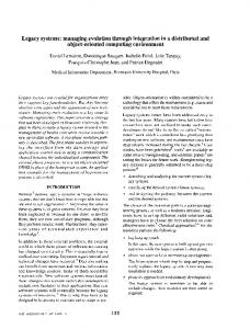
4. OOPAR Environment Fig. 1. Computational element with corresponding graphical element.

3.4. Graphical Grid: Post-Processing High Resolution Approximations Most finite element programs use linear or bilinear approximation spaces. As such, post-processing is limited to the interpolation of the post-processed variables at the nodes of the finite element grid. In cases where the interpolation of the solution uses high order polynomials, the linear interpolation of the solution over the nodes of the geometric grid ignores the resolution of the computed approximation. No post-processor can receive coefficients associated with high order polynomials for post-processing: such coefficients would need to be supplemented with a description of the construction of the high order shape functions. The proposed solution is to create a graphical grid, which implements a logical uniform refinement on the original finite element grid. To each computational element in the computational grid, a graphical element is created. To each computational node a graphical node is created. Figures 1 and 2 illustrate the concept of graphical elements and nodes. When a graphical node writes its data to a file, it writes the post-processing data corresponding to all individual points. When a graphical element writes its connectivity to a grid, it writes the connectivity of all elements it contains.

Fig. 2. Computational nodes with corresponding graphical nodes.

Parallel programming is not difficult. Most researchers who start using message passing libraries are amazed how simple it is to transfer messages between processors. On the other hand, parallel programming increases the dimension of complexity of the program: the parallel programming paradigm requires the use of new concepts such as synchronism and barriers, and if asynchronous communication is used, the execution path of the program becomes non-deterministic. Several object oriented interfaces exist for parallel programming [19]. Most of these environments are either a C⫹⫹ interface to the message passing interface, or are applied to the parallelisation of a particular algorithm [20,21]. The object oriented interface to parallel programming presented develops a new paradigm which offers an interface to the message passing interface library, a distributed data model and a parallel task concept. Its intention is to be coupled to the TMatrix and PZ environments, to allow both environments to be executed on parallel computers. Using structured programming, the author has developed several programs for parallel finite element computing, and has noticed the following bottlenecks: 1. The impact of the message passing interface on the code structure is very great. If data structures of any level of complexity need to be shared between processors, sending and receiving routines become very complex. 2. It is virtually impossible to escape from synchronised message passing. When a process sends a message to another process, the receiving process needs to know beforehand which data structure will be received. 3. Parallel programs are of the branch and join type, with obvious synchronisation barriers and sequential code bottlenecks. Coding complexity inhibits any other approach. This section describes and abstraction layers which are OOPAR. These layers should be asynchronous parallel programs,

motivates several implemented in sufficient to write transmitting com-

70

P. R. B. Devloo

plex data structures between processes. The different abstraction layers are 쐌 Abstraction of message passing – Communication Manager. 쐌 Abstraction of the distributed pointer mechanism. 쐌 Administration of distributed objects – Data Manager. 쐌 Tasks. 쐌 Administration of tasks – Task Manager. 4.1. Abstraction of the Message Passing Interface: Communication Manager Both PVM and MPI allow only simple data structures to be transmitted between processes. Each send or receive procedure corresponds to a single data item. When working with object oriented programming languages, data structures tend to become increasingly complex. Both PVM and MPI allow the user to pack objects of different type within a buffer which is transmitted as a single message. The packing of data structures as a stream of bytes and subsequent object recomposing is often referred to as object serialisation. Within OOPAR, serialised classes are derived from the base class TSaveable. The TSaveable class defines the interface which derived classes need to implement. This interface is virtual void Pack (TSendbuffer *);

which will pack the data contained within the object to the send buffer virtual void Unpack (TReceivebuffer *bf, int &position);

which converts the stream of bytes into the original object. Note that the Pack and Unpack may be called recursively. To initiate the object recombination based on a stream of bytes, a class recombination method is associated with each serialised class. The first integer of transmitted method identifies the procedure needed to recompose the object. The interface of the procedure is TSaveable *Restore int &position);

(TReceiveBuffer

*bf,

A pointer to this function can be found by calling GetRestore: typedef TSaveable *(*) (TReceiveBuffer *bf, int &position) TRestoreFunction; TRestoreFunction GetRestore (long classid); GetRestore returns a pointer to the procedure

which will recompose an object of a type identified by an ID. Using the above described procedure, it is possible to transmit objects of arbitrary types between processes. The problem with which the programmer is now faced is: What is the destination of the received objects? When a process receives an object of a given type, what does it need to do with it? After an object has been transmitted to another process, how can the original process refer to the transmitted object. These problems are addressed in the next abstraction layer. 4.2. Abstraction of the Distributed Pointer Mechanism Within a sequential or multi-threaded environment, object are identified by their address. Within a parallel computer with distributed memory, the pointer mechanism cannot be used anymore to identify the objects. To overcome this problem, the OOPAR introduces the distributed data object, which assigns a unique identity with each object which needs to be shared among processes. With this mechanism, the user of OOPAR can associate a serialised object with a serialised object, transmit the distributed data object to another process and use it within a parallel algorithm. The distributed data objects are managed by the Data Manager, which stores them in a binary tree for rapid access. A version number with each distributed data object: this allows to associated a state with each object. The next pending problem is: there is a distributed data model, but the operations/algorithms which will be performed on this distributed data must still be hard coded. This means that each process must know what type of data objects will be transmitted, and which operations need to be performed on these. This model still doesn’t allow to write general purpose parallel software. 4.3. Tasks A task is an object which, through its virtual execute method, will access/transform distributed data objects. Each task object belongs to a class derived from TTask which in turn is derived from TSaveable. Therefore, task objects can be transmitted from one process to another. In order to execute, task objects depend upon accessing distributed data objects. Two types of access are distinguished: read access and write access. The task object is not supposed to modify

Object Oriented Tools for Scientific Computing

a distributed data object to which it has read access; it will generally modify distributed data objects to which it has write access. The task which modifies a distributed data object will generally increase its version number. The execution sequence of a parallel program now consists in creating task objects of the appropriate type, and giving the appropriate data dependency to each task object. There are still two elements missing: 1. As tasks depend upon data access, it is conceivable that two task objects will want to access a distributed data object simultaneously. Distributed data objects exist, but there is no arbitration scheme which will decide which task object has access to which data. This arbitration will be implemented within the Data Manager. 2. Several tasks can be created simultaneously. Some tasks can be set up for execution, while others need to be queued till their data dependency is satisfied. The set of tasks is administered by the Task Manager. 4.4. Administering Distributed Data Objects: The Data Manager The Data Manager assigns a unique identity to serialised objects. After a serialised object has been submitted to the Data Manager, the Data Manager will administer all access to that object. One process is considered as the owner of a distributed data object. Data access at other processes is granted at the process level. Many processes can access a distribute data object simultaneously, but only one process can have write access to a distributed data object. The process which has write access to the object is considered owner of the object. Requests for data access are queued at each object. If a data access requested by a task can be satisfied, the Data Manager notifies the task object and passes it the pointer to the requested object. After a task terminates, it notifies the Data Manager it doesn’t need the data access anymore. The Data Manager can then grant access to another task or process which queued a request. 4.5. Administering Task Objects: The Task Manager The execution sequence of a parallel program within OOPAR generally follows the execution sequence of the data flow paradigm: a set of tasks are queued

71

for execution, each one depending on a particular version of a distributed data object. As the object is gradually modified by the execution of the tasks, the parallel algorithm is executed. Tasks are queued within the Task Manager. The Task Manager verifies whether an queued task has received all data accesses it requested and, if affirmative, sets the task up for execution. Tasks execute in separate threads, which implies that data communication is done separately from the execution of the parallel program. This also implies that several tasks can be executed in parallel within a single process, which makes OOPAR suitable for shared memory machines as well. Within OOPAR, the user does not have to worry about the explicit transfer of objects: objects are transmitted between processes in response to access requests of tasks or other processes. Tasks can execute on any process, which implies that OOPAR is an appropriate environment to experiment with dynamic load balancing strategies.

5. Conclusions Within the effort of the author to develop object oriented scientific software, three different environments have been distinguished: an environment for linear algebra, an environment for the development of finite element software and an environment for developing parallel software. The development philosophy of each environment is considered more important that the environments itself. As such, the matrix environment is extendible to include new matrix storage forms, the finite element environment separates the geometric map from the definition of the interpolation space, and from the definition of the system of partial differential equations and the parallel environment implements the concept of distributed data objects and tasks.

Acknowledgements The development of the object oriented tools described above is the fruit of collaborative work between the author, colleagues and students. The financial support of CNPq and FAPESP has also been crucial to buy equipment and pay scholarships to faculty and students. Finally, the author extends his gratitude to the administration and support team of CENAPAD who administer the access to the IBM/SP2 computer. The many constructive comments of the referee also helped to improve the quality of this contribution.

72

References 1. Devloo, P., Alves, J. (1992) An object oriented approach to finite element programming (phase 1) a system independent windowing environment for developing interactive scientific software. Advances in Engineering Software and Workstations, 14, 41–46 2. Dongarra, J., Lumsdaine A., Niu, X., Pozo, R., Remington, K. (1994) Sparse matrix libraries in C⫹⫹ for high performance architectures. Proceedings of the Second Annual Object-Oriented Numerics Conference (OON-SKI’94), April 24–27, 122–138 3. Dongarra, J. J., Duff, I. S., Sorensen, D. C., der Vorst, H. A. V. (1993) Solving Linear Systems on Vector and Shared Memory Computers. Society for Industrial and Applied Mathematics, 3600 University City Science Center, Philadelphia PA 19104–2688, second ed 4. Barrett, R., Berry, M., Chan, T., Demmel, F., Donato, J., Dongarra, J., Eijkhout, V., Pozo, R., Romine, C. der Vorst, H. V. (1994) Templates for the Solution of Linear Systems: Building Blocks for Iterative Methods, SIAM 5. Santana, M., Devloo, P. (1998) Behavior of a preconditioner implemented using hierarchical bases. In: Computational Mechanics, New Trends and Applications (E. D. S. Idelsohn, E. On˜ate, eds), Fourth World Congress on Computational Mechanics (IV WCCM), Buenos Aires, Argentina 6. Devloo, P. R. B., Santana, M. L. M. (1996) Desenvolvimento de algoritmos de sub estruturac¸a˜o para elementos finitos. Proceedings of the 6th Brazilian Congress of Engineering and Thermal Sciences, Floriano´polis, SC, Brasil, November, 505–510 7. Klapka, I., Demonceau, T., Cardona, A., Ge´radin, M. (1994) Object Oriented Finite Elements Led by Interactive Executor. Technical Report SA-175, LTAS, 10 8. Klapka, I., Cardona, A. (1994) Design of a new finite element programming environnement. Engineering Computations, 11 9. Haney, S., Crotinger, J., Karmesin, S., Smith, S. (1999) Easy expression templates using PETE, the portable expression template engine. Dr Dobbs Journal. www.ddj.com

P. R. B. Devloo

10. Zimmermann, T., Bomme, P., Eyheramendy, D., Vernier, L., Commend, S. (1998) Aspects of an objectoriented finite element environment. Computers & Structures, 68, 1–16 11. Mackie, R. (1998) An object-oriented approach to fully interactive finite element software. Advances in Engineering Software, 29, 139–149 12. Donescu, P., Laursen, T. (1996) A generalized objectoriented approach to solving ordinary and partial differential equations using finite elements. Finite Elements in Analysis and Design, 22, 93–107 13. Devloo, P.R.B. (1997) PZ: An object oriented environment for scientific programming. Computer Methods in Applied Mechanics and Engineering, 150, 133–153 14. Menezes, F., Slhessarenko, L., Devloo, P. (1998) Tridimensional analysis of buildings using an oriented object environment. In Computational Mechanics, New Trends and Applications. (E. D. S. Idelsohn, E. On˜ate, eds) Fourth World Congress on Computational Mechanics (IV WCCM), Buenos Aires, Argentina 15. Menezes, F., Devloo, P., Slhessarenko, L. (1997) Extensa˜o da teoria de reissner mindlin para cascas, in Estruturas e Fundac¸o˜es, H.M.C.C. Antunes, ed., XXVIII Jornadas Sul-Americanas de Engenharia Estrutural, Sa˜o Carlos, Brasil, 1033–1042 16. Menezes, F., Devloo, P., Slhessarenko, L. (1997) Aproximac¸a˜o de arcos utilizando uma extensa˜o da teoria de Timoshenko. Proceedings XVIII CILAMCE – Congresso Ibero Latino Americano de Me´todos Computacionais Para Engenharia 17. Shephard, M. S., Dey, S., Flaherty, J. E. (1997) A straight forward structure to construct shape functions for variable p-order meshes. Computer Methods in Applied Mechanics and Engineering, 147, 209–233 18. Devloo, P., Bravo, C., Pavanello, R. (1998) On the definition of high order shape functions for finite elements. Work in progress 19. Dongarra, B. T. J. J. (1994) Environments and Tools for Parallel Scientific Computing. Philadelphia, SIAM 20. Hsieh, S., Modak, S., Sotelino, E. (1995) Objectoriented parallel programming tools for structural engineering applications. Computing Systems in Engineering, 6, 533–548 21. Mukunda, G., Sotelino, E., Hsieh, S. (1998) Distributed finite element computations using object-oriented techniques. Engineering with Computers, 14, 59–72