Abstract. Object recognition is an important research field of computer vision and
has its ... known as Genetic algorithm (GA) for solving the optimization problem.
IJCSI International Journal of Computer Science Issues, Vol. 10, Issue 5, No 2, September 2013 ISSN (Print): 1694-0814 | ISSN (Online): 1694-0784 www.IJCSI.org
55
OBJECT RECOGNITION USING PARTICLE SWARM OPTIMIZATION AND GENETIC ALGORITHM Mahmood ul Hassan 1, M. Sarfraz 2, Abdelrahman osman 3 and Muteb Alruwaili 4 1, 3, 4
Department of Computer Science, College of Science and Arts. Al Jouf University Tabarjal, Jouf, Saudi Arabia 2 Department of Information Science, Kuwait University P.O. Box 5969, Safat 13060, Kuwait
Abstract Object recognition is an important research field of computer vision and has its application in a broad range of problems including image retrieval, compression, surveillance and medical diagnostics. The main goal of the object recognition problem is to recognize the objects of the same type even when they are viewed from different viewpoints. This goal, however, remains a challenge for computer vision to recognize objects having invariant features such as translation, rotation and scaling. Shape descriptors like Fourier and Moments are invariant with respect to transformation, rotation and scaling. Particle swarm optimization (PSO) is a population based soft computing technique. Particle Swarm Optimization technique shares numerous similarities with evolutionary computation techniques such as Genetic Algorithms (GA). One of the most important tasks regarding to object recognition is how to find number of descriptors of a given object. The query that arises is what is the optimum number of descriptors to be used with maximum recognition rate? , Are descriptors having equal importance? Such reasons signify the importance of these descriptors and also selecting the best descriptor by applying optimization technique. We have introduced an evolutionary optimization technique known as Genetic algorithm (GA) for solving the optimization problem. GA assigns, for each of these descriptors, a weighting factor that reflects the relative importance of that descriptor. Keywords: Object recognition, Fourier descriptors, Genetic algorithm, ORGA (Object Recognition using Genetic Algorithm), PSO.
1. Introduction Object recognition in computer vision is the task of finding a given object in an image or video sequence. Humans recognize a multitude of objects in images with little effort, despite the fact that the image of the objects may vary somewhat in different viewpoints, in many different sizes / scale or even when they are translated or rotated. There are various disciplines of everyday life, including security, health, post, defense, surveillance, etc., where the issue of object recognition needs to be tackled
fastly and accurately. Shape descriptors [1 - 6] like Fourier can be classified by their invariance with respect to the transformations allowed in the associated shape definition. These descriptors are invariant with respect to congruency, meaning that congruent shapes (shapes that could be translated, rotated) will have the same descriptor. These descriptors describe the features of an object to uniquely represent the shape of an object. In this paper we are using Genetic Algorithm technique on Fourier Descriptors then we will compare the results with PSO [6] that have been frequently used as features for image processing, remote sensing, shape recognition and classification. These Descriptors can provide characteristics of an object that uniquely represent its shape. This paper has used Fourier descriptors, with different combinations, for the recognition of objects captured by an imaging system which may transform, make noise or can have occlusion in the images. An extensive experimental study, similar to the moment invariants [7], has been made using various similarity measures in the process of recognition. These measures include Euclidean Measure, Percentage error, Log of Euclidean and Log of square of Euclidean. Comparative study of various cases has provided very interesting observations which may be quite useful for the researchers as well as practitioners working for imaging and computer vision problem solving. Although the whole study has been made for bitmap images, but it can be easily extended to gray level images. From the analysis and results using Fourier Descriptors, the following questions arise: What is the optimum number of descriptors to be used? Are these descriptors of equal importance? To answer these questions, the problem of selecting the best descriptors has been formulated as an optimization problem. Genetic algorithm (GA) technique has been mapped and used successfully to have an object recognition system using minimal number of Fourier Descriptors. The goal of the proposed optimization technique is to select the most helpful descriptors that will maximize the recognition rate. The proposed method will assign, for each of these
Copyright (c) 2013 International Journal of Computer Science Issues. All Rights Reserved.
IJCSI International Journal of Computer Science Issues, Vol. 10, Issue 5, No 2, September 2013 ISSN (Print): 1694-0814 | ISSN (Online): 1694-0784 www.IJCSI.org
descriptors, a weighting factor that reflects the relative importance of that descriptor. The outline of the remainder of the paper is as follows. Getting of bitmap images and their outline is discussed in Sections 2 and 3 respectively. The concepts of similarity measures are explained in Section 4. Fourier theory is explained in Section 5. Section 6 explains the detail of PSO. Detail of proposed technique is explained in Section 7. Proposed algorithm is explained in section 8. Detailed experimental study and analyses are made in Section 9 whereas Section 10 deals with interesting observations during the experimental study. Finally, Section 11 concludes the paper as well as touches some future work.
56
attempted for experimental studies, are Euclidean Distance (ED), Log of Euclidean Distance (LED), Log of Square of Euclidean Distance (LSED) and Percentage Error (PE).
n
a i b i
1.
2
(Euclidean Distance (ED)) (1)
i 1
n
2.
a i
b i
(Percentage Error (PE))
(2)
i 1
3. LED log
n
a i b i
2
Log of Euclidean
i 1
2. Getting Bitmap Image Bitmap image of a character can be obtained by creating a bitmap character on some program like Paint or Adobe Photoshop. Alternatively an image drawn on paper can scan and store it as bitmap. We used both methods. The quality of bitmap image obtained directly from electronic device depends on the resolution of device, type of image (e.g. bmp, jpeg, tiff etc), number of bits selected to store the image etc. The quality of scanned image depends on factors such as quality of image on paper, scanner and attributes set during scanning.
Distance (LED)
4.
n 2 LSED log a i b i i1
(3)
Log of Square
of Euclidean Distance (LSED)
(4)
In this study, n is the number of FDs considered, a (i) is the ith FD of the template image, and b (i) is the ith FD of the test image. A tolerable threshold is selected to decide a test object recognized. This threshold is checked against the least value of the selected similarity measure.
3. Finding Boundary In order to find boundary of bitmap image, first its chain code is extracted [8, 9]. Chain codes are a notation for recording the list of edge points along a contour. The chain code specifies the direction of a contour at each edge in the edge. From chain coded curve, boundary of the image is found [10]. The selection of Boundary Points is base on their corner strength and contour fluctuations. The input to our boundary detection algorithm is a bitmap image
Fig. 1 (a) Bitmap image
(b) outline of the image
Figure 1(a) shows the bitmap image of a character. Figure 1(b) shows detected boundary of the image of Figure 1(a).
4. Similarity Measures We implement four different simple classifiers that calculate different similarity measures of the corresponding Fourier descriptors of the input shape and each of the shapes contained in the database. The similarity measures,
5. Fourier Theory To characterize objects we use features that remain invariant to translation, rotation and small modification of the object‟s aspect. The invariant Fourier descriptors of the boundary [11-13] of the object can be used to identify an input shape, independent on the position or size of the shape in the image. Fourier transform theory has played a major role in image processing for many years. It is a commonly used tool in all types of signal processing and is defined both for one and two-dimensional functions. In the scope of this research, the Fourier transform technique is used for shape description in the form of Fourier descriptors. The Fourier descriptor is a widely used all-purpose shape description and recognition technique. The shape descriptors generated from the Fourier coefficients numerically describe shapes and are normalized to make them independent of translation, scale and rotation. These Fourier descriptor values produced by the Fourier transformation of a given image represent the shape of the object in the frequency domain. The lower frequency descriptors store the general information of the shape and
Copyright (c) 2013 International Journal of Computer Science Issues. All Rights Reserved.
IJCSI International Journal of Computer Science Issues, Vol. 10, Issue 5, No 2, September 2013 ISSN (Print): 1694-0814 | ISSN (Online): 1694-0784 www.IJCSI.org
57
the higher frequency the smaller details. Therefore, the lower frequency components of the Fourier descriptors define a rough shape of the original object The Fourier transform theory can be applied in different ways for shape description. One method works on the change in orientation angle as the shape outline is traversed. But in our research the following procedure was implemented, the boundary of the image is treated as lying in the complex plane. So the row and column co-ordinates of each point on the boundary can be expressed as a complex number.
Fig. 2 General architecture of PSO
The advantage of using the Fourier transform is in its invariant properties. Rotating the object merely causes a phase change to occur, and the same phase change is caused to all the components.
PSO starts working with a population of random solutions. Each particle move towards its fittest solution it has achieved so far. As PSO has its memory so it stores the value of fitness. PSO has also a global best value which is known as gbest from where the overall best value is stored.
The simple geometric transformations of the Fourier transform are as follows:
At each step PSO changes the velocity of each particle in the direction of pbest and gbest.
Translation: u(n) +t a(k) +tδ(k)
Rotation : u(n)ejθ a(k)ejθ
Scaling: su(n) sa(k)
Starting point: u (n-t) a (k) ej2∏tk/N.
6. Particle Swarm Optimization (PSO) Particle swarm optimization (PSO) is a population based soft computing technique developed by Dr. Eberhart and Dr. Kennedy in 1995. Particle Swarm Optimization technique shares numerous similarities with evolutionary computation techniques such as Genetic Algorithms (GA). PSO starts initialization with a population of random solutions and searches for optimum solution by updating generations. However, if we compare PSO with GA then unlike GA, PSO has no operators such as crossover and mutation. In PSO, the possible solutions, called particles, move through the problem space by following the current optimum particles. In PSO initial steps for recognition of an object is to check the noise from the image. If it found the noise then remove it from the image with the help of noise removing algorithm. After cleaning the noise, boundary is calculated with the help of chain code [14]. Now apply fast Fourier transformation on the boundary points to get descriptors. Now from here PSO assigns weight to each descriptor.
This soft computing technique has numerous advantages over traditional techniques. It starts working with population of solutions from where it selects the best one while traditional does not work in similar way. They start searching with holding single solution. So in this regard PSO produced much better results as compare to traditional ones.
7. Optimization of the Feature Vector using Genetic algorithm From the previous analysis and results, the following questions arise: What is the optimum number of descriptors to be used? Are these descriptors of equal importance? To answer these questions, the problem of selecting the best descriptors can be formulated as an optimization problem. The goal of the optimization is to select the most helpful descriptors that will maximize the recognition rate and to assign for each of these descriptors a weighting factor that reflects the relative importance of that descriptor.
7.1 Objective Function Since the problem of selecting the best descriptors can be formulated as an optimization problem, one need to define an objective function. The objective function, in this case, is made up of the following two terms:
The recognition rate,
The number of useful descriptors.
In other words, it is required to maximize the recognition rate using the minimum number of descriptors. The
Copyright (c) 2013 International Journal of Computer Science Issues. All Rights Reserved.
IJCSI International Journal of Computer Science Issues, Vol. 10, Issue 5, No 2, September 2013 ISSN (Print): 1694-0814 | ISSN (Online): 1694-0784 www.IJCSI.org
function of the optimization algorithm is to assign a weight wi for every descriptor so that the objective function is optimized, where wi belongs to [0,1].
value or no conspicuous improvement is to be observed to the fitness after certain iterations. 1.
The mathematical formulation of the objective function is defined as follows:
J H * min PE ,
(5)
Where H is the number of hits (the number of correct matches), and PE is the percentage of errors of all the training images for a given set of weights, and is a factor that is adjusted according to the relative importance of the min(PE) term. In most of the simulations, 0.7 is experienced as best case most of the time The first term, the objective function Eq. (5), makes GA search for the weights that result in the highest recognition rate and the second term makes the GA reach to the highest recognition with the minimum number of descriptors.
Generally, GA works as follows: a population of individual is initialized where each individual represents a potential solution to the problem. The quality of each solution is evaluated using a fitness function. A selection process is applied during each iteration of GA in order to form a new population. The selection process is biased towards the fitter individuals to insure that they will be a part of new population. Individuals are altered using two main operators of GA which are crossover and mutation. This procedure is repeated until the potential solution is reached. The best solution found is expected to be a near optimum solution [Michalewicz 1996].
7.3 Steps of the GA
Initialization: - The first step for genetic algorithm in the optimization process is initialization. In this step various parameters are initialized to their desired value. In current simulation we have set the following parameters.
Bias is set between 0 and 0.2.
Number of iterations are 25 but we have also set the stopping criteria. If the stopping criteria meet during the specified iterations the simulation ends otherwise it goes for the number of iterations specified.
Numbers of trials are used in between 10 to 15.
Stopping criteria is also set which depends on the hits used in the simulation.
2.
Evaluate fitness function:- The second step of Genetic algorithm is to calculate the fitness of each individual. For this purpose we assign weights to all set of individuals, so we calculate fitness against each individual. This Fitness represents the importance of attached weights, and is given by:
7.2 Genetic Algorithm GA was introduced first in 1960 by John Holland [15]. GA is also known as evolutionary algorithm (EA). Evolutionary algorithms are general-purpose stochastic methods simulating natural selection and evolution in the biological world. GA differ from other optimization methods, such as PSO, Simulated Annealing, in the fact that GA maintain a population of potential solutions to the problem, and not just one solution.
58
f 1 min( PE )
Where f represents the fitness value and PE is the percentage error of all the training objects for a given set of weights. 3.
Apply crossover: - Crossover is the most important operator of GA. Initially crossover is applied on randomly selected population (weights).
4. Apply mutation: - If stopping criteria matched then terminate else apply mutation on newly created population and check for hits. If current hit ratio is better than previous, population will be replaced with newly generated population, otherwise step (vi) will be repeated until best hit ratio is achieved. Now again check here for stopping criteria, if found then terminate otherwise start searching from the start.
8. Proposed Algorithm Initialization:
Genetic algorithm work as follows: at first population is created randomly, which satisfies the environmental constraint of problem. There are four steps in the Genetic algorithm. The first step is initialization. Other three steps “evaluation of fitness function, crossover and mutation” are inside a main loop. The execution of these steps is in a sequence until the fittest population arrives at a maximum
Set stopping criteria Set no of iterations (Stopping criteria) Set no of trials Set threshold to compute goodness 1.
Load database of descriptors.
2.
Initialize an array of particles with random values
Copyright (c) 2013 International Journal of Computer Science Issues. All Rights Reserved.
IJCSI International Journal of Computer Science Issues, Vol. 10, Issue 5, No 2, September 2013 ISSN (Print): 1694-0814 | ISSN (Online): 1694-0784 www.IJCSI.org
as initial weights. 3.
Evaluate goodness & check the stopping criteria.
4.
If stopping criteria does not meet then apply crossover on the weights & check for hits. If current hits are better than previous, replace new population with previous and store the hits.
5.
Repeat for all Childs after crossover.
6.
Check the stopping criteria.
7.
Apply mutation on each particle & check for hits. If current hits are better than previous then replace.
8.
Check for stopping criteria.
9.
If best hit meet stopping criteria then stop Else
Several experiments have been attempted to use GA to search for the optimum descriptor weights. These experiments are summarized in Tables 2 to 7. In these tables, “No. of FDs” means the number of Fourier descriptors used in the optimization process. For example, if this number is F, the GA is supposed to search for F weights, a single weight for a single FD, which maximize the recognition rate with the minimum number of descriptors. Table 1: Optimized weights for different numbers of Fourier descriptors. Experiment
Recognized Object Classifiers
.6
.9
.7
5
X
X
X
O
X, O, N
11
7
6
6
11
0.19
0.149
0.135
0.116
0.141
0.21
0.1489
0.528
0.1457
0.7
0.2
0.1488
0.415
0.0841
0.0118
0.771
0.858
0.924
0.4544
0.0675
0.897
0.941
0.942
0.4418
0.277
0.96
0.7027
0.935
0.3533
0.4099
0.864
0.5466
considered
Optimized Weights (GA)
Fig. 3 Pictorial description of the proposed technique
Figure 3 shows the complete description of the proposed technique.
0.1592
0.1939
0.6508
0.9048
0.411
Experiment
The genetic algorithm can be found in the current literature at many places.
1
2
3
4
5
X
X
X
O
X, O, N
11
7
6
6
11
95%
93.33%
95%
90%
98.33%
No. Training set* No. of FDs Rec
The proposed GA–based approach was implemented using MATLAB 7.1.0 (simulator) for performance evaluation of proposed technique. In our implementation, the Bias is set between 0-0.2, number of iterations are 25, and the numbers of trials are used in between 10 to 15. The search process stops either desired hits are achieved or it exceeds from the specified number of iterations.
0.7313
Table 2: Recognition rates for different numbers of Fourier descriptors using Euclidean distance (PSO)
X
tion
In this section we will compare proposed work with one of the most important soft computing technique known as Particle Swarm Optimization (PSO).
0.7568
Table 1 shows the optimized weight for GA.
ogni
9. Results and Analysis
0.7199
0.88
e
Database of FDs
.4
4
No. of FDs
Optimized Weights obtained
Input Shape
.3
3
Training set
End
Descriptors
2
Rat
11. If stopping criteria doesn‟t meet for number of trials then go to step2.
.5
1
No.
10. Repeat step 3 to 9
Contour Shape
59
Copyright (c) 2013 International Journal of Computer Science Issues. All Rights Reserved.
N
93.75%
93.75%
87.5
87.5%
87.5%
O
23.33
25%
20%
20%
25%
Table 3. Recognition rates for different numbers of Fourier descriptors using Euclidean distance (ORGA)
Percentage success rate
IJCSI International Journal of Computer Science Issues, Vol. 10, Issue 5, No 2, September 2013 ISSN (Print): 1694-0814 | ISSN (Online): 1694-0784 www.IJCSI.org
60
100 80
Recognition Rate X(GA) Recognition Rate X(PSO)
60 40 20 0 X 11
3
4
5
Training set
X
X
X
O
X,O,N
No of FDs
11
7
6
6
11
100
98.33
96.67
93.33
93.33
X N
100
100
100
100
93.75
O
26.67
23.33
21.67
20
16.67
„Object recognition using genetic algorithm (ORGA)‟ In the first experiment when a database of 60 transformed objects, in Table 3, was considered, one can see a much better recognition results than in Table 2. ORGA recognizes object 100% in some of the cases. For transformed, noisy and occluded objects, the recognition rate is 100%, 100% and 26.67% as compare to PSO. Experiment 2, when considered for 7 weighted FDs, shows generally, much better results than using 7 weighted FDs in PSO. In case of transformed, noisy and occluded objects, the recognition rate is significant as compare to PSO. Experiment 3, when considered for 6 weighted FDs, shows generally, much better results than using 6 weighted FDs in PSO. Recognition rate for transformed, noisy and occluded objects are better than PSO. Experiment 4, when considered for 6 weighted FDs and the training set is considered for occluded objects, shows generally, much better results than using 6 weighted FDs in PSO. Experiment 5, when considered for 11 weighted FDs and the training set is considered for mixed objects (combination of transformed, noisy and occluded objects), shows much better improvement in case of noisy objects.
X
O
X,O,N
7
6
6
11
Training set, No of FDs
Fig. 3 Comparative graph for transformed objects (using ED)
Percentage success rate
2
100 80 Recognition Rate N(GA)
60
Recognition Rate N(PSO)
40 20 0 X
X
X
O
X,O,N
6
7
11
6
11
Training set, No of FDs
Fig. 4 Comparative graph for noisy objects (using ED)
Percentage success rate
1
Recognition Rate
Experiment No
X
35 30 25
Recognition Rate N(GA)
20
Recognition Rate N(PSO)
15 10 5 0 X 6
X
X
O
O
7
11
6
11
X,O,N 11
Training set, No of FDs
Fig. 5 Comparative graph for occluded objects (using ED)
Copyright (c) 2013 International Journal of Computer Science Issues. All Rights Reserved.
IJCSI International Journal of Computer Science Issues, Vol. 10, Issue 5, No 2, September 2013 ISSN (Print): 1694-0814 | ISSN (Online): 1694-0784 www.IJCSI.org
Experiment
1
2
3
4
Percentage success rate
Table 4: Recognition rates for different numbers of Fourier descriptors using log of square of Euclidean distance. (PSO) 5
No. X
Rate
Recognition
No. of FDs
X
X
O
11
7
6
6
11
X
95%
96.67%
96.67%
90%
98.33%
N
93.75%
93.75%
87.5
93.75%
93.75%
O
21.67
16.67%
20%
20%
25%
2
3
60
Recognition Rate N(GA)
40
Recognition Rate N(PSO)
20 0
4
X
X
X
O
X,O,N
11
7
6
6
11
Fig. 7 Comparative graph for noisy objects (using LSED)
Table 5: Recognition rates for different numbers of Fourier descriptors using log of square of Euclidean distance. (ORGA) 1
80
Training set, No of FDs
Table 4 shows the recognition rates for the different number of Fourier descriptors by using PSO.
Experiment No
100
X, O, N
30
Percentage success rate
Training set
61
25 20
Recognition Rate N(GA)
15
Recognition Rate N(PSO)
10 5 0
5
X
X
X
O
X,O,N
11
7
6
6
11
Training set, No of FDs
X
X
X
O
X,O,N
No of FDs
11
7
6
6
11
X
100
98.33
96.67
93.33
93.33
N
100
100
100
100
93.75
O
26.67
23.33
21.67
20
16.67
Recognition Rate
Training set
Fig. 8 Comparative graph for occluded objects (using LSED)
Recognition rate for LED is same as in LSED. Table 6: Recognition rates for different numbers of Fourier descriptors using Percentage error (PSO) Experiment
1
2
3
4
5
Training set
X
X
X
O
X, O, N
No. of FDs
11
7
6
6
11
X
75%
70%
65%
73.33%
66.67%
N
81.25%
81.25%
68.75%
87.5%
75%
O
18.33%
6.67%
13.33%
13.33%
8.33%
Percentage success rate
Table 4 shows the recognition rates for the different number of Fourier descriptors by using GA. In the first experiment when a database of 60 transformed objects, in Table 4 and 5, was considered, results of ORGA are better than PSO. ORGA recognizes object 100% in some of the cases. For transformed, noisy and occluded objects, the recognition rate is much better than PSO. 100
Recognition Rate
No.
80 60
Recognition Rate X(GA)
40
Recognition Rate X(PSO)
Table 6 shows the recognition rates for the different number of Fourier descriptors by using PSO.
20 0 X
X
X
O
X,O,N
11
7
6
6
11
Training set, No of FDs
Fig. 6 Comparative graph for transformed objects (using LSED)
Copyright (c) 2013 International Journal of Computer Science Issues. All Rights Reserved.
Table 7: Recognition rates for different numbers of Fourier descriptors using Percentage error (ORGA) Experiment
1
2
3
4
5
No. Training set
X
X
X
O
X, O, N
No. of FDs
11
7
6
6
11
Percentage success rate
IJCSI International Journal of Computer Science Issues, Vol. 10, Issue 5, No 2, September 2013 ISSN (Print): 1694-0814 | ISSN (Online): 1694-0784 www.IJCSI.org
62
20 15
Recognition Rate X(GA)
10
Recognition Rate X(PSO)
5 0 X
X
X
O
X,O,N
11
7
6
6
11
Recognition Rate
Training set, No of FDs
X
80%
80%
75%
78.33%
72%
N
87.5%
87.5%
87.5%
87.5%
81.25%
O
15%
7%
11.67%
13.33%
16.67%
Fig. 11 Comparative graph for occluded objects (PE)
10. Some observations
Percentage success rate
In all experiments when a database of 60 transformed objects, in Table 7, was considered, results of ORGA (proposed approach) for transformed, noisy and occluded objects are better than PSO in Table 6. 100 80 60
Recognition Rate X(GA)
40
Recognition Rate X(PSO)
20 0 X
X
X
O
X,O,N
11
7
6
6
11
Training set, No of FDs
Percentage success rate
Fig. 9 Comparative graph for transformed objects (PE)
100 80 60
Recognition Rate X(GA)
40
Recognition Rate X(PSO)
20 0 X
X
X
O
X,O,N
11
7
6
6
11
Training set, No of FDs
Fig. 10 Comparative graph for noisy objects (PE)
Here are some observations for the whole discussion in the paper: The Fourier descriptors of the boundary are robust to similarity transformations. Fourier descriptors were found to be able to recognize at a higher rate if we use nine or more Fourier descriptors. This trend continues when the size of the database is increased from 15 to 45 to 60. Most cumulative combinations of Fourier descriptors are able to recognize most of the images correctly for samples without noise or occlusion. It is noted that if an image is recognized, it is recognized by most cumulative combinations of Fourier descriptors, and if it is not recognized, then it is not recognized by almost all cumulative combinations of Fourier descriptors. Noise (salt and pepper) with density of ten percent has a minimal effect on the recognition ability of Fourier descriptors. When we use eight or more Fourier descriptors add ten percent salt and pepper noise to the images, the accuracy level does not drop. Noise of type salt and pepper with ten percent density has similar effect on Fourier descriptors such that the decrease in recognition is noticeable but very slightly. Occlusion brings down the recognition rate of Fourier descriptors from 80-90 percent to around 20%. The Fourier descriptors show a steady increase in accuracy level as the number of Fourier descriptors used increases. It then stabilizes at same level for nine to eleven descriptors. Fourier descriptors perform very poorly in the
Copyright (c) 2013 International Journal of Computer Science Issues. All Rights Reserved.
IJCSI International Journal of Computer Science Issues, Vol. 10, Issue 5, No 2, September 2013 ISSN (Print): 1694-0814 | ISSN (Online): 1694-0784 www.IJCSI.org
(a)
presence of occlusion in the image. The occlusion is a big issue in object recognition problem, especially, when we use Fourier descriptors. Since the method works on the boundary of edge of objects, any distortion on the shape will be affected to the recognition process. This occlusion may happen to some part of the object see Fig. 12(a). The remaining part of the object can be used for recognition process and we can guess the correct object according to the excellent part. So, it is recommended to divide the template data (the boundary of object) to four parts depending on x and y axis, see Fig. 12(b). Then, each of this part can be computed according to the Fourier approach. We can take the test object and can also divide its boundary on the axis. Each of quarter will be computed and compared to database, see Fig. 12(c). The test object will be recognized as agreeing of its parts on the specific object. Using GA to find the most suitable descriptors and to assign weights for these descriptors improves dramatically the recognition rate using the least number of descriptors. (b)
(c)
63
used are all bitmapped images, further investigations are being done with some more complex images. It can be seen that, using PE with FDs results in less efficient performance than using ED. Moreover, increasing the number of FDs does not necessarily guarantee a better performance. The images that have to be recognized but failed to be recognized by most of the FD combinations are to be analyzed further. This leads to the theory of optimization to find out appropriate features or attributes in the image that made it difficult to be recognized. The methodology of GA has been utilized successfully for this purpose. Using GA, to find the most suitable descriptors and to assign weights for these descriptors, improved dramatically the recognition rate using the least number of descriptors. In future, author would like to treat the problem as multiobjective optimization method, also try to enhance the GA by tuning different parameters to maximize the recognition rate while minimizing the number of descriptors. Acknowledgments This work has been supported by AL Jouf University, Saudi Arabia under the Supervision of Dr Muhammad Sarfraz.
References
Fig. 12 Occlusion suggestion: Each quarter can be computed and compared to database.
11. Conclusion and Future work This work has been reported to make a practical study of the Fourier descriptors to the application of Object Recognition. The implementation was done on a LAPTOP using MATLAB 7.1.0. The ultimate results have variations depending upon the selection of number of FDs, similarity transformations, noise, occlusion, and data size. The variety of similarity measures and different combinations of FD features, used in the process, make a difference to the recognition rate.. Four similarity measures, including ED, and PE, LED and LSED provided different recognition results. The images
[1] David G. Lowe, “Object Recognition from Local Scale-Invariant Features”, Vancouver, B.C.,V6T 1Z4, Canada [2] Weina Ge,” OBJECT RECOGNITION: BEYOND VISION”, Ph.D. Candidate, Computer Science and Engineering, College of Engineering [3] M. Sarfraz, “Object Recognition using Fourier Descriptors: Some Experiments and Observations”, Proceedings of the International Conference on Computer Graphics, Imaging and Visualisation 2006 [4] G. H. Granlund, “Fourier Preprocessing for hand print character recognition”, IEEE Trans. Computers, Vol C-21, Febr. 1972, pp. 195-201. [5] A Project led by Julien Boeuf and Pascal Belin, and supervised by Henri http://www.tsi.enst.fr/tsi/enseignement/ressources/mti/desc ript_fourier [6] M. Sarfraz, and A.T.A. Al-Awami, (2006), “Object Recognition using Particle Swarm Optimization on Fourier Descriptors”, Proceedings of the 11th Online World Conference on Sof Computing in Industrial Applications (WSC11) September 18th - October 06th, 2006 - On the Internet (World
Copyright (c) 2013 International Journal of Computer Science Issues. All Rights Reserved.
IJCSI International Journal of Computer Science Issues, Vol. 10, Issue 5, No 2, September 2013 ISSN (Print): 1694-0814 | ISSN (Online): 1694-0784 www.IJCSI.org
[7] M. Sarfraz, Object Recognition using Moments: Object Recognition using Moments: Some Experiments and Observations: Geometric Modeling and Imaging – New Advances, Sarfraz, [8] Avrahami, G., Pratt, V.: Sub-pixel edge detection in character digitization. In: Raster Imaging and Digital Typography II, pp. 54–64 (1991) [9] Hou, Z.J., Wei, G.W.: A new approach to edge detection. Pattern Recognition 35, 1559–1570 (2002) [10] Richard, N., Gilbert, T.: Extraction of Dominant Points by estimation of the contour fluctuations. Pattern Recognition 35, 1447–1462 (2002) [11] G. Avrahami and V. Pratt. Sub-pixel edge detection in character digitization. Raster Imaging and Digital Typography II, pp. 54-64, 1991. [12] Hou Z. J., Wei G. W., A new approach to edge detection, Pattern Recognition Vol. 35, pp.15591570, 2002. [13] N. Richard, T. Gilbert, Extraction of Dominant Points by estimation of the contour fluctuations, Pattern Recognition Vol. 35, pp. 1447-1462, 2002. [14] H. Freeman and A. Saghri. Generalized chain codes for planar curves. In Proceedings of the 4th International joint conference on Pattern Recognition, pages 701-703, Kyoto, Japan, November 7-10-1978 [15] D. Goldberg, Genetic algorithms in search, optimization and machine learning. Addison-Wesley, 1989. Mahmood ul Hassan was born in Mansehra, Pakistan, in 1985. He received the B.S. degree from Hazara university and M.S. degree from COMSATS University Abbottabad, Pakistan From 2008 to 2010, he was a Research Assistant in COMSATS Abbottabad, Pakistan. Since 2010, he has been Lecturer in Computer department at Al Jouf University, Saudi Arabia. He has six International Journal publications and four International conference publications. Dr Muhammad Sarfaraz was born in Pakistan. He is the member of IEEE and the IEEE Compter Society. Currently he is the faculty member of Kuwait university. He has a number of many journal and conference publications. He is also the author of a number of books related to the field of computer science. Dr Abdel Rehman osman was the faculty member of Al Jouf University Saudi Arabia from 2010 to 2012. He has a number of many journal and conference publications. He is also the author of a number of books related to the field of computer science.
Muteb Alruwaili is the faculty member of Al Jouf University Saudi Arabia from 2011 to present. He has a number of many journal and conference publications.
Copyright (c) 2013 International Journal of Computer Science Issues. All Rights Reserved.
64