The Astrophysical Journal Letters, 810:L10 (6pp), 2015 September 1
doi:10.1088/2041-8205/810/1/L10
© 2015. The American Astronomical Society. All rights reserved.
OBSERVATIONS AND NUMERICAL MODELING OF THE JOVIAN RIBBON R. G. Cosentino1, A. Simon2, R. Morales-Juberias1, and K. M. Sayanagi3 1
New Mexico Institute of Mining and Technology, Socorro, NM 87801, USA;
[email protected] 2 Solar System Exploration Div., NASA/GSFC, Greenbelt, MD 20771, USA 3 Hampton University, Hampton, VA 23668, USA Received 2015 May 22; accepted 2015 July 28; published 2015 August 25
ABSTRACT Multiple wavelength observations made by the Hubble Space Telescope in early 2007 show the presence of a wavy, high-contrast feature in Jupiter’s atmosphere near 30°N. The “Jovian Ribbon,” best seen at 410 nm, irregularly undulates in latitude and is time-variable in appearance. A meridional intensity gradient algorithm was applied to the observations to track the Ribbon’s contour. Spectral analysis of the contour revealed that the Ribbon’s structure is a combination of several wavenumbers ranging from k = 8–40. The Ribbon is a dynamic structure that has been observed to have spectral power for dominant wavenumbers which vary over a time period of one month. The presence of the Ribbon correlates with periods when the velocity of the westward jet at the same location is highest. We conducted numerical simulations to investigate the stability of westward jets of varying speed, vertical shear, and background static stability to different perturbations. A Ribbon-like morphology was best reproduced with a 35 ms−1 westward jet that decreases in amplitude for pressures greater than 700 hPa and a background static stability of N = 0.005 s−1 perturbed by heat pulses constrained to latitudes south of 30°N. Additionally, the simulated feature had wavenumbers that qualitatively matched observations and evolved throughout the simulation reproducing the Jovian Ribbon’s dynamic structure. Key words: planets and satellites: atmospheres – planets and satellites: general – planets and satellites: physical evolution Supporting material: animation 1. INTRODUCTION
Jupiter and Saturn have shown how the properties of some observed waves are dependent on the conditions of the background flow and static stability of the atmosphere (Gierasch 2004; Sayanagi et al. 2010). We explored the effects of vertical wind shear, static stability, and location of perturbations to determine their impact on reproducing a Ribbon-like feature. Zonal wind profiles from the Hubble Space Telescope (HST), Voyager 2, and Cassini observations provided a range of testable westward jet velocities near 30°N. Simulation results were compared to our benchmark 2007 HST observations of the Ribbon’s structure and spectral signature.
Planetary scale waves are found in the Jovian atmosphere at several latitudes, such as circumpolar waves at 50°N, 57°S, and 67°N and S (Barrado-Izagirre et al. 2008) and Rossby waves at 7°N and S (Simon-Miller et al. 2012; Choi et al. 2013, and references therein) planetographic latitude.4 These waves manifest themselves as evenly spaced longitudinal intensity patterns in visible and infrared observations. The spectral analysis of these wave patterns reveals specific, dominant planetary wavenumbers that do not noticeably change over time. At 30°N another planetary scale wave-like feature exists, hereafter called the Jovian Ribbon, which has multiple wave modes as shown in Figure 1. The multiple wavenumbers combine to manifest themselves as irregular wave-like undulations in latitude of the surrounding cloud morphology. Hereafter, we describe irregular undulations as a wavy cloud morphology that does not have a dominant wavenumber and consequently has a chaotic morphology. The Jovian Ribbon shares some similarities with a feature on Saturn that is located near 47°N, the Saturnian Ribbon (Smith et al. 1982). Both features reside at extra-tropical latitudes in the northern hemispheres of their respective planets, and their structures appear as irregular wave-like cloud opacity differences that vary in latitude. However, these features are different in that while the Saturnian Ribbon is located near a strong eastward jet of 140 ms−1, the Jovian Ribbon is associated with a weak westward jet with a maximum observed speed of 35 ms−1. We aim to understand what underlying atmospheric conditions and processes favor the genesis of the Jovian Ribbon’s irregular cloud morphology near 30°N. Previous studies of 4
2. OBSERVATIONS Observations from Voyager, HST, and Cassini were used to make longitudinal maps of the region near 30°N with resolutions near 0 °. 1 as shown in Figure 1. The Ribbon’s presence seems to correlate with periods when the westward jet velocity at 30°N is greatest. The wind profiles from Voyager and HST were obtained by manual measurements, using the smallest visible tracers (Simon-Miller & Gierasch 2010) while Cassini utilized correlation (Porco et al. 2003). The feature is very prominent in the HST 2007 observations. The HST and Cassini observations in 1995 and 2000 show that powerful convective events affect the region’s cloud morphology, and it is uncertain if our view is obscured or if the Ribbon’s continuity is disrupted. Observations have also shown that the westward jet near 30° N varies in speed and location as a function of time. Fourteen HST observations were used to measure the zonal winds between 1994 July and 2008 June. The westward jet’s velocity where the Ribbon is located was observed to increase from 15 ms−1 in 1997 April to 35 ms−1 in 1998 July over a time period of almost 400 days. We found the westward jet’s peak
Latitudes are planetographic unless otherwise noted.
1
The Astrophysical Journal Letters, 810:L10 (6pp), 2015 September 1
Cosentino et al.
Figure 1. Zonal wind profiles (solid black line, left column) for the westward jet near 30°N. Dashed zonal profiles represent the uncertainties from each observation (Voyager uncertainties are too small to be seen). Vertical dashed lines shown at −35 and −25 ms−1 show the limits of variation in the zonal velocity. Corresponding observation maps (right column) covering 120° longitude of Jupiter made from blue (400 to 450 nm) images with 0 °. 1 resolution. A movie made from the Voyager observations shows that the phase of the large-scale Ribbon-like morphology near 30°N is nearly stationary, while smaller cloud features move along the Ribbon’s outline, and this indicates that the westward zonal jet is truly meandering in latitude. (An animation of this figure is available.)
was centered at a mean latitude of 31°N with an average velocity of 25 ms−1. We based our analysis of the Ribbon’s structure on HST observations made in 2007 February and March. Spectral analysis of longitudinal Fast Fourier Transform (FFT) scans at the center latitude near 31°N revealed the presence of several wave modes. However, FFT scans of the jet’s center and latitudes north or south revealed that the Ribbon’s spectral signature depended on the scanned latitude. Specifically, the relative power of wave modes varied with latitude, indicating that a more robust method for characterizing the Ribbon’s structure was needed to compare different observations to each other and to our simulations. The Jovian Ribbon’s structure is most prominent when we take the ratio of HST blue (410 nm) and red (673 nm) filters. The Ribbon’s high-contrast wave-like pattern between regions of light and dark is likely due to differences in local cloud properties (e.g., opacity, altitude). We developed an algorithm to analyze the meridional intensity gradient for all longitudes within a latitudinal band that enclosed the Ribbon. For each longitude, the local extremum of the intensity gradient was found and its latitude recorded, thus obtaining the contour of the Ribbon. Figures 2(a) and (c) show the algorithm’s output over-plotted on the 2007 observations. We used this contour to perform spectral analysis of the Ribbon’s structure; the dominant wavenumbers for 2007 February are k = 10, 13, 20, and 25, while for 2007 March they are k = 8, 15, 31, and 36. (Zonal planetary wavenumber k is defined as the number of complete waves encompassed within the planetary circumference at a specific latitude.) We tested the sensitivity of the spectral signature to the removal of outlying points as described below. First we smoothed the contour with a moving average of varying lengths over the image’s 3600 pixel longitude span.
Figure 2(a) shows the smoothing results with an 11 pixel moving average, corresponding to a smoothing length of 1 °. 1 which would remove spectral features with wavenumbers over k = 100. Next, we found an average latitude for each one degree longitude and set a limit from the average latitude to remove outliers. We tested different longitude binning lengths and limits away from the average latitude and found that the spectral signature was largely insensitive to these changes. Figure 2(c) shows the retrieved signal using a longitude binning length of 1° and latitude limits of 0 °. 5 from the average. Spectral analysis to the final Ribbon contours revealed similar spectral power signatures for each method. The insensitivity of the spectral analysis produced by each method leads us to believe this algorithm is robust and more accurate than FFT’s longitudinal scans when attempting to quantify the structure of a Ribbon-like feature for multiple observations. 3. MODELING We used the Explicit Planetary Isentropic-Coordinate General Circulation Model which integrates the primitive equations (Dowling et al. 1998) to simulate the Jovian Ribbon. We used a resolution of ≈0 °. 6, or ≈660 km at 30°N, for a longitude and latitude domain of 300 by 18°. There are 20 vertical layers from 10,000 to 0.1 hPa, with layers above 50 hPa set to dampen vertically propagating waves (i.e., sponge layers), and a sixth order hyperviscosity term was used to eliminate numerical modes. The atmospheric stability was varied using different values of the Brunt–Väisälä frequency (N) in modified temperature versus pressure profiles. We used the observed temperatures above 500 hPa from Seiff et al. (1998), and below 500 hPa we calculated the temperature profile for different constant values of N. We created Gaussian zonal wind profiles to span the 2
The Astrophysical Journal Letters, 810:L10 (6pp), 2015 September 1
Cosentino et al.
Figure 2. Two observations of the Jovian Ribbon produced from two HST filters ratio: blue (410 nm) over red (673 nm). Panel (a) shows intensity gradient algorithm output after a moving average smoothing window length of 11 pixels, and panel (c) shows the 1° binned longitude averages with a half degree tolerance outlining (light red) with removed points (red). The dashed black lines represent the latitudes scanned by the algorithm. The spectral analysis for the Ribbon’s raw data, smoothed with the moving averge, and retained points are shown in panels (b) and (d), respectively. Panel (e) shows a potential vorticity grayscale map produced from a simulation near 800 hPa. Highlighted is the jet’s path (RV0) and spectral analysis for days 301 and 336 is shown in panel (f).
westward jet’s velocity range, where the wind speed and FWHM are tunable parameters. For all simulations the jet’s speed approached zero in altitudes higher than 700 hPa to match the observed vertical wind shear (Gierasch et al. 1986). The vertical wind profile for pressures greater than 700 hPa was varied to explore how shear affected the development of a Ribbon-like feature. We varied the shear to be either constant with depth (Uz = 0), decreasing to near zero at the bottom model layer (Uz < 0 ), or increasing to maintain a continuous shear matching the winds above (Uz > 0 ).
We perturbed the westward jet with small, stochastic Gaussian heat pulses that vary in intensity, horizontal size, duration, and time between successive pulses, simulating the effects produced from convection. Based on Galileo observations of Jupiter’s thunderstorms, Gierasch et al. (2000) estimated the heat release to be 5 × 10¹⁵ W from a storm that covered an area 1000 km by 1000 km and vertically extended one scale height. Our random heat pulses, on average, have that same size and yield a heat release of 2 × 10¹⁵ W for our maximum heating rate of 1.0 J kg−1 s−1. Also, at any one
3
The Astrophysical Journal Letters, 810:L10 (6pp), 2015 September 1
Cosentino et al.
Figure 3. Time evolution of the Ribbon-like feature from simulation days 250 to 350. Spectral analysis of RV0 is shown on the left, while on the right, the jet path RV0 line is plotted every other day for all longitudes. Table 1 Atmospheric Stability, Shear, and Wind Velocity N (s-1)
Shear (Uz)
U0 = 15 (ms−1)
U0 = 25 (ms−1)
U0 = 35 (ms−1)
0.003 0.004 0.005 0.006 0.007 0.003 0.004 0.005 0.006 0.007 0.003 0.004 0.005 0.006 0.007
Constant Constant Constant Constant Constant Decreasing Decreasing Decreasing Decreasing Decreasing Increasing Increasing Increasing Increasing Increasing
NF NF NF NF VS NF NF NF NF VS NF NF NF NF VS
VS VS VS VS VS NF VS VS VS VS NF NF NF VS VS
VS VS VS VS VS W R R VS VS NF NF NF VS VS
for cloud morphology in our study. We looked for a strong PV gradient in our simulations of a Ribbon-like feature which would be consistent with our observational analysis. We then performed spectral analysis on the relative vorticity contour equal to zero (RV0), which approximated the jet’s path as done in Sayanagi et al. (2010). We identified Ribbon-like features that met the following criteria: i. PV field near 800 hPa has a high gradient near 30°N; ii. spectral analysis of RV0 near 800 hPa has at least three prominent wave modes with k < 50 that are not harmonics; iii. RV0 is visibly irregular and persists for 100 days; iv. spectral power transfers between multiple modes on a timescale similar to that of observations, ≈1 month; v. PV field away from 30°N remains mostly flat. Table 1 displays the results of our initial parameter space exploration in which the heat pulses were scattered over the entire domain. We found little development of instabilities with low jet velocities, reaffirming that the Ribbon’s presence is correlated with periods when the westward jet velocity is greatest. Ribbon-like features were only produced for simulations with jet velocities of 35 ms−1, Uz < 0 , and N = 0.004 or 0.005 s-1. Only these cases met criteria i–v listed above. The shear below 700 hPa for Uz < 0 was −12.65 ms−1 per scale height and decreased the zonal wind to 1.3 ms−1 at the model bottom. Results in Table 1 had a timestep of dt = 40 s. We repeated simulations for Uz < 0 to test numerical convergence and found similar Ribbon-like features for dt = 20, 30, 50, and 60 s. We chose the case with N = 0.005 s-1 to be further explored because the meridional extent of RV0 was greater than the case with N = 0.004 s-1. We ran additional simulations to test the sensitivity of these results to changes in the location of the perturbations. When the perturbations were located at the westward jet’s center latitude, vortex street (VS) appeared more quickly than when the pulses were located at all latitudes. A VS is a
Note. Space of parameters sampled by our initial exploration of instabilities in the westward jet. The results are described as: R—Ribbon-like, meeting criteria i–v, VS—vortex street, series of alternating cyclones and anticyclones, W— wave, a strong PV gradient dominated by a single wavenumber, and NF—for nearly featureless PV fields.
time on Jupiter, there are as many as 50 thunderstorms (Ingersoll 2013), which in our model domain, would translate to 4 concurrent storms. We limit our pulse occurrences to one per Jovian day. Therefore, our perturbations represent a conservative estimate of the amount of energy injected into the atmosphere from convection. Different latitudinal domains for the perturbation’s location were tested as described in the following section. 4. RESULTS As done by Morales-Juberías & Dowling (2013), the potential vorticity (PV) field near 800 hPa was used as a proxy 4
The Astrophysical Journal Letters, 810:L10 (6pp), 2015 September 1
Cosentino et al.
Figure 4. Top panels (a) and (b) display HST images (410 nm) of a “streamer” feature associated with Jovian Ribbon observations. Panel (c) shows a simulated Ribbon with PV contours 5-7 m−1 s−1 apart and panel (d) as a grayscale map.
only one or two wavenumbers. The chaotic nature of this Ribbon-like feature is shown on the right side of Figure 3, where several small features in RV0 move coherently for only brief periods of time. Both HST observations in 2007 show “wispy white tail” features that are reminiscent of “streamers” in Earth’s atmosphere (Krüger et al. 2005), where the sharpening PV gradient is a result of wave breaking (Figures 4(a) and (b)). In our model, the RV0 contour has noticeable “pinching” at day 282 as shown in Figure 4(c). The PV field shown as a grayscale image in Figure 4(d) enhances this feature and displays similarities between the model output and the HST observations.
longitudinal staggered series of cyclones and anticyclones. We were only able to generate a Ribbon-like feature that persisted throughout the entire simulation (400 days) when the perturbations’ location was constrained to latitudes between 25° and 29°N. This latitudinal domain corresponds to cyclonic shear on the side of the jet where lightning associated with convection has been observed (Little et al. 1999; Dyudina et al. 2004). Figure 2(e) shows the PV field and RV0 contour at day 301 for this case. As shown in the figure, the PV field in this case has an irregular gradient near 30N while remaining mostly flat away from that latitude. The RV0 contour traces the westward jet core and is similar in appearance to the strong PV gradient. Spectral analysis of the RV0 contour reveals multiple wavenumbers below k = 50 and shows spectral power transfer over a period of 41 days similar to the 2007 observations. The evolution of this Ribbon-like structure for days 250–350 is shown in Figure 3. The left side of Figure 3 shows the presence of multiple wave modes that transfer spectral power over time, suggesting the Ribbon-like feature is not defined by
5. DISCUSSION The westward jet near 30N is barotropically unstable, violating the Rayleigh–Kuo criterion that compares the latitudinal gradient of the Coriolis parameter to the second 5
The Astrophysical Journal Letters, 810:L10 (6pp), 2015 September 1
Cosentino et al.
derivative of the zonal velocity with respect to latitude (Vallis 2006). Simulations in Table 1, where Uz = 0, primarily investigated barotropic instability on the westward jet’s evolution. All of these cases resulted in VS. Since the observed Jovian Ribbon is not associated with a set of vortices, this would rule out barotropic instability as the primary generating mechanism. The meridional gradient of PV changes sign in the model domain and violates the Charney–Stern criterion for baroclinic instability (Vallis 2006). Ribbon-like features were produced with Uz < 0 , and this is consistent with theoretical work for unstable westward jets with growing modes on Jupiter (Gierasch 2004). We showed that when Uz < 0 , the westward jet must have a significant baroclinic component influencing the instability to evolve into a Ribbon-like feature instead of a VS. Additionally, we found that the role of the atmosphere’s static stability, N, promotes the development of a VS for more stable atmospheres, while less stable atmospheres produce more wave-like structures. We demonstrated that our simulated Jovian Ribbon is consistent with two independent sets of observations. First, its presence is correlated with periods when the westward jet’s velocity is greatest, verified by our ability to reproduce Ribbonlike features for jet velocities of only 35 ms−1. Second, we showed that the simulated Ribbon is best reproduced when perturbations are located in a region of cyclonic shear at latitudes where lightning and storms occur. This suggests that lateral perturbations in Jupiter’s atmosphere, most likely high frequency gravity waves from local convective events or geostrophic adjustment of storms, produces a forced wave that we observe as the Jovian Ribbon. Previous modeling of the Saturnian Ribbon investigated instabilities and saturation processes of the 47N jet where this feature is located with Uz = 0 (Sayanagi et al. 2010). Those results showed noticeable patches of PV at 45°N. A flanking westward jet is located at 40°N, and as our results indicate, the absence of vertical shear leads to the development of PV patches. In late 2016, the Juno spacecraft and the Cassini proximal mission will measure the shape of the gravity fields of Jupiter and Saturn, from which the deep structure of the zonal winds could be revealed. Dynamical phenomena like the Jovian and
Saturnian Ribbons serve as benchmarks in computational models, and their comparative analysis can also illustrate the underlying dynamical structure of these atmospheres. This work was based on observations made with the NASA/ ESA Hubble Space Telescope under programs GO/DD 5313, 5642, 6009, 6452, 7616, 8148, 8405, 10782, 11096, 11102, 11310, and 11498, publicly available through the Mikulski Archive for Space Telescopes. The Space Telescope Science Institute is operated by the Association of Universities for Research in Astronomy, Inc., under NASA contract NAS526555. All Voyager data are available through the Planetary Data System. Computational resources were provided by New Mexico Institute of Mining and Technology and by Computational and Information Systems Laboratory at National Center for Atmospheric Research. Yellowstone: IBM iDataPlex System. Boulder, CO. This work was partially supported by NASA PATM grant # NNX14AH47G to A.S. K.M.S. was supported in part by NASA OPR grant # NNX12AR38G. Facilities: HST, Voyager II, Cassini.
REFERENCES Barrado-Izagirre, N., Sánchez-Lavega, A., Pérez-Hoyos, S., & Hueso, R. 2008, Icar, 194, 173 Choi, D. S., Showman, A. P., Vasavada, A. R., & Simon-Miller, A. A. 2013, Icar, 223, 832 Dowling, T. E., Fischer, A. S., Gierasch, P. J., et al. 1998, Icar, 132, 221 Dyudina, U. A., Del Genio, A. D., Ingersoll, A. P., et al. 2004, Icar, 172, 24 Gierasch, P. J. 2004, Icar, 167, 212 Gierasch, P. J., Ingersoll, A. P., Banfield, D., et al. 2000, Natur, 403, 628 Gierasch, P. J., Magalhaes, J. A., & Conrath, B. J. 1986, Icar, 67, 456 Ingersoll, A. P. 2013, Planetary Climates (Princeton, NJ: Princeton Univ. Press) Krüger, K., Langematz, U., Grenfell, J. L., & Labitzke, K. 2005, ACP, 5, 547 Little, B., Anger, C. D., Ingersoll, A. P., et al. 1999, Icar, 142, 306 Morales-Juberías, R., & Dowling, T. E. 2013, Icar, 225, 216 Porco, C. C., West, R. A., McEwen, A., et al. 2003, Sci, 299, 1541 Sayanagi, K. M., Morales-Juberías, R., & Ingersoll, A. P. 2010, JAtS, 67, 2658 Seiff, A., Kirk, D. B., Knight, T. C. D., et al. 1998, JGR, 103, 22857 Simon-Miller, A. A., & Gierasch, P. J. 2010, Icar, 210, 258 Simon-Miller, A. A., Rogers, J. H., Gierasch, P. J., et al. 2012, Icar, 218, 817 Smith, B. A., Soderblom, L., Batson, R. M., et al. 1982, Sci, 215, 504 Vallis, G. K. 2006, in Atmospheric and Oceanic Fluid Dynamics, ed. G. K. Vallis (Cambridge: Cambridge Univ. Press), 247
6